Mechatronics for Safety, Security and Dependability in a New Era - Arai and Arai Part 13 docx

344
Ch70-I044963.fm Page 344 Friday, July 28, 2006 1:50 PM
Ch70-I044963.fm Page 344 Friday, July 28,2006 1:50 PM
344
M(s)
F(s)
-A
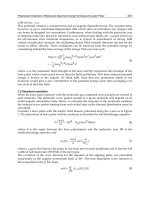
Fig. 1. The block diagram of the feedback-type active noise cancellation system.
The transfer function of the acoustic environment (the plant) must also be taken into account when
designing the filters that define the operating frequency range. In the present case the plant consists of
the earcup, the mechanical construction of the hearing protector, the microphone, the loudspeaker, and
the head and ear of the user. As with any system with negative feedback and high gain, the active noise
control system may become unstable under certain circumstances. A block diagram of an active noise
cancellation system is shown in Figure 1. S
n
is the noise signal, M(s), F(s), -A and L(s) are the transfer
functions of the error microphone, the filter, the amplifier, and the loudspeaker (the secondary source),
respectively.
A loud low-frequency signal can saturate the amplifier. When this occurs, no signal can pass through it
without becoming distorted. For example, when a low frequency tone saturates the amplifier, a higher
frequency tone also becomes distorted. For example, head movement and walking cause changes in the
pressure of the air inside the earcup. These infrasound pressure variations can be extremely large in
magnitude when compared with audible sounds. The microphone also converts these strong infrasound
signals into electric signals, which may get distorted because of the supply voltage limitations. The
movement of the earcup may also cause instability. For example, an adaptive ANC headset developed
by Rafaely maintained stability during minor changes in the fit, but became unstable when the headset
was suddenly moved or subjected to an impact (Rafaely 1997).
In addition, the sensors of an active noise control system may be saturated if the noise level exceeds
the dynamic range of the sensors. The saturation generates harmonic distortion (Kuo 2004). However,
in the present case the only sensor is located in the quiet zone. Tt is, therefore, unlikely that the sensor
will be saturated. Instead, the loudspeaker and amplifiers are more likely to be saturated because of the

higher signal level.
THE IMPLEMENTED PROTOTYPE
A prototype of an active noise cancellation hearing protector was implemented according to the block
diagram shown in Figure 1. The prototype was implemented using analog feedback-type system. The
operating frequency range is defined by high-pass and low-pass filters. The low-pass filter was
designed in order to ensure stable operation at the upper end of the frequency range, whether the
earcup is tightly fit, partially open, or fully open.
An electronic solution to the saturation problem described in the previous chapter was developed. An
automatic gain control (AGC) circuit, which adjusts the amount of active attenuation, was developed
(Oinonen 2004). When a loud low frequency signal is present, the amount of active attenuation is
reduced in order to avoid saturation.
Stability at higher frequencies was ensured by careful design of the low-pass filter and acoustic plant.
The filter was adjusted so that the device will be stable with tight or loose fit. The goal in designing the
345
Ch70-I044963.fm Page 345 Friday, July 28, 2006 1:50 PM
Ch70-I044963.fm Page 345 Friday, July 28,2006 1:50 PM
345
acoustic plant was to avoid sharp resonance peaks in the transfer function. Any cavities, which could
store acoustic energy were avoided.
The developed prototype was installed inside a high-quality passive hearing protector. The secondary
source was installed in a small enclosure, and the error sensor was placed near the secondary source.
The complete secondary source and error sensor -assembly was installed so that it is located near the
ear. The assembly described above was installed in both earcups of the hearing protector. A 3.6 V
lithium-ion -battery was installed inside one earcup and the ANC controller was installed inside the
other earcup.
IN-EAR MEASUREMENTS
The performance of the implemented prototype was measured using in-ear method. The sound
pressure level at the entrance of the ear canal was measured without hearing protection, with passive
hearing protection and with active hearing protection.
A Sennheiser KE 4-211-1 electret microphone capsule was placed at the entrance of the ear canal. The

microphone was connected to a self-made batteiy-powered microphone pre-amplifier. The amplified
signal was recorded by a Sony DCD-D8 portable DAT recorder and analysed using a Briiel & Kjaer
2260 Investigator sound level meter. Fast time constant and A-weighting were used. The
measurements were made in a room equipped with sound-absorptive material covering the walls and
ceiling. Two different kinds of noise stimuli were used. The first stimulus was a 30-second sample of
pink noise generated by a self-made digital pink noise generator. The other stimulus was a 30-second
sound recorded inside a moving tank, and it was played by a Sony ZA5ES DAT player. The signal
sources were connected to an active speaker system via an AMC Stereo Preamplifier 1100. The active
speaker system consists of two Genelec 1030A two-way monitors and one Genelec 1092A subwoofer
unit.
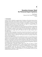
The first stimulus was pink noise. The sound pressure levels without hearing protection (solid line),
with passive hearing protection (dotted line) and with active hearing protection (dash-dot -line) are
presented in Figure 2a. A sound sample of a moving tank served as the second stimulus. The sound
pressure levels without hearing protection (solid line), with passive hearing protection (dotted line) and
with active hearing protection (dash-dot -line) are shown in Figure 2b.
The dynamic range of the device was also tested. Pink noise was used as a stimulus and the sound
pressure level was increased gradually from 80 dB SPL to 100 dB SPL. It was clear that the effect of
a) 90
10 F(Hz)
F(Hz)
10"
10'
Fig. 2. Third octave band levels of the noise with pink noise (a) and tank noise (b).
346
Ch70-I044963.fm Page 346 Friday, July 28, 2006 1:50 PM
Ch70-I044963.fm Page 346 Friday, July 28,2006 1:50 PM
346
the active attenuation gradually disappeared when the AGC circuit reduced the gain of the controller.
Audible distortion was not detected until the sound pressure level reached 97 dB SPL inside the
earcup. However, with loose fit between the hearing protector and the head, distortion could be heard

at lower sound pressure levels.
The in-ear measurement results show that the developed device is able to actively attenuate low
frequency noise up to a maximum of 20 dB. This is a significant improvement in the low frequency
performance of a hearing protector. The measured active attenuation is almost same for both stimuli.
The automatic gain control circuit reduces the active attenuation when needed, which makes the device
more usable in high noise level environments. The drawback of the gain reduction is that active
attenuation performance is reduced at the same time. The device also improves comfort and speech
intelligibility because it reduces significantly the low frequency boom, which is typical of passive
hearing protectors due to their poor low frequency attenuation. Because the prototype improves low
frequency noise attenuation, it reduces the risk of hearing loss and thus improves safety. Although the
AGC circuit reduces distortion and extends the dynamic range of the device, further research is still
needed for very high SPL environments.
CONCLUSIONS
One problem associated with active hearing protectors is that a loud low frequency sound can saturate
the system, which is heard as distortion. A prototype of an active noise cancellation hearing protector
had been developed earlier, and now special attention was paid to improving the comfort and stability
of the device. As a solution, an automatic gain control circuit was incorporated, and both acoustical
and electrical designs were improved in order to ensure stability. In-ear measurements were made. The
measurement results show that the developed prototype significantly improves the low frequency
attenuation of a passive hearing protector. The listening tests demonstrated that the AGC circuit makes
the device more comfortable to use. Further, there was no sign of instability.
ACKNOWLEDGEMENTS
This work was supported by Oy Silenta Electronics Ltd, a Finnish hearing protector manufacturer and
TEKES,
The National technology agency of Finland.
REFERENCES
1.
Rafaely B. (1997). Feedback Control of Sound. Ph. D. Thesis, University of
Southampton,
UK,

2.
Kuo S.M., Wu H. Chen F., and Gunnala M.R. (2004). Saturation Effects in Active Noise
Control Systems. IEEE Transactions on Circuits and Systems-I: Regular Papers 51:6, 1163 -
1171.
3.
Oinonen M.K., Raittinen H.J., and Kivikoski M.A. (2004). An Automatic Gain Control for an
Active Noise Cancellation Hearing Protector. Active 2004 - The 2004 International Symposium
on Active Control of Sound and Vibration, Williamsburg, VA USA.
347
Ch71-I044963.fm Page 347 Tuesday, August 1, 2006 4:45 PM
Ch71-I044963.fm Page 347 Tuesday, August 1, 2006 4:45 PM
347
SUPPRESSING MECHANICAL VIBRATIONS IN A PMLSM USING
FEEDFORWARD COMPENSATION AND STATE ESTIMATES
M. J. Hirvonen and H. Handroos
Institute of Mechatronics and Virtual Engineering, Department of
Mechanical Engineering, Lappeenranta University of Technology
P.O.Box 20, FIN-53851 Lappeenranta, FINLAND
ABSTRACT
The load control method for suppressing mechanical vibrations in a Permanent Magnet Linear
Synchronous Motor (PMLSM) application is postulated in this study. The control method is based on
the load acceleration feedback, which is estimated from the velocity signal of a linear motor using the
Kalman Filter. The linear motor itself is controlled by a conventional PI -velocity controller, and the
vibration of the mass is suppressed from an outer control loop using feed forward acceleration
compensation. The proposed method is robust in all conditions, and is suitable for contact less
applications e.g. laser cutters. The algorithm is first designed in the simulation program, and then
implemented in the physical linear motor using a DSP application. The results of the responses are
presented.
KEYWORDS
Acceleration Compensation, Kalman Filter, Linear Motor, Velocity Control, Vibration Suppression

INTRODUCTION
Nowadays fast dynamic servomotors are becoming quite common in several machine automation
areas.
This sets new demands on mechanisms connected to motors, because it can easily lead to
vibration problems due to fast dynamics. On the other hand the non-linear effects caused by motor and
machine mechanism frequently reduce servo stability, which diminishes the controller's ability to
predict and maintain speed. As a result, the examination of vibrations that are formed in a motor as
well as of the mechanism's natural frequencies, has become important.
The traditional approach to the dynamic analysis of mechanisms and machines is based on the
assumption that systems are composed of rigid bodies. However, when a mechanism operates in high-
speed conditions, the rigid-body assumption is no longer valid and the load should be considered
flexible. The flexibility of a mechanism causes a disturbing velocity difference between reference- and
load velocity, especially in the fast transient state.
348
Ch71-I044963.fm Page 348 Tuesday, August 1, 2006 4:45 PM
Ch71-I044963.fm Page 348 Tuesday, August 1, 2006 4:45 PM
348
Conventionally the motor control is assumed to be a velocity controller of a motor. In that case the
vibrations of the tool mechanism, reel, gripper or any apparatus connected to the motor are not taken
into account. This might reduce the capability of the machine system to carry out its assignment and
impair the lifetime of the equipment. Nonetheless, it is usually more important to know how the load
of the motor behaves.
There are two complementary methods to improve the dynamic behaviour of the machine system. The
first is to make the mechanism more rigid, but this method usually makes the response slower. The
second is to take the dynamic behaviour of the mechanism into account in the control strategy. The
latter method is of interest to us. Motion control technologies have been widely used in industrial
applications. Due to the fact that good technologies allow for high productivity and products of high
quality, the study of motion control is a significant topic.
The aim of the proposed controller is to drive the load to a reference in such a way that the load
follows the desired value as rapidly and as accurately as possible, but without awkward vibration. One

of the most traditional methods to suppress resonance in the electromechanical system is to allow only
small and slow changes in the reference command. For example different kinds of filters are used in a
reference signal to suppress mechanical vibrations. Dumetz et al. (2001) have studied bi-quad and low
pass filters in a control loop but also as a reference filter. The closed loop filter makes possible to
compensate poles and zeros of the transfer function from the motor side, and the reference filter
compensates poles of the transfer function in the load side. Another widely used filter for vibration
suppression is the Notch filter (Ellis et al., 2000). The drawback of the filtering is the low sensitivity to
parameter variations and also this method reduces the dynamical properties of a servo system.
A more promising method is to use acceleration compensation to suppress load vibration. Tn this
method the motor is controlled by a simple PT -controller and load acceleration can be measured or
estimated and used as a compensation feedback. Kang et al. (2000) and Lee et al. (1999) have used
this kind of a method successfully in the vibration control of elevators. The weakness of using
acceleration feedback is that the signal is usually very noisy. If the system is observable, it is possible
to estimate the state variables that are not directly accessible to measurement using the measurement
data from the state variables that are accessible. By using these state-variable estimates rather than
their measured values one can usually achieve an acceptable performance. State-variable estimates
may in some circumstances even be preferable to direct measurements, because the errors of the
instruments that provide these measurements may be larger than the errors in estimating these
variables.
CONTROLLER DESIGN
Tn control system design, the mechanism can usually be simplified for a 2-dof system, when only the
first fundamental natural mode is taken into account. The two-mass-spring model of the linear motor
system is introduced in Figure 1.
m
M
\-m-
Figure 1: Two-mass-spring model of the PMLSM.
349
Ch71-I044963.fm Page 349 Tuesday, August 1, 2006 4:45 PM
Ch71-I044963.fm Page 349 Tuesday, August 1, 2006 4:45 PM

349
The transfer function from the controller force F to the load velocity x
2
is the following:
bs + k
F
jS' +b(m
l
+m
2
)s
2
+k(m
l
+m
2
)s
(1)
where b is the damping constant, k is the spring constant, and m\ and ni2 are motor and load mass,
respectively. Tn theory, the conventional linear controller (Pl/PTD) can suppress the vibration of the
load in the linear system. There are small gain margins in the root locus where the system is stable.
However, when controlling the load by a simple PT controller, the velocity becomes unstable very
quickly when the gains are increased. The physical linear motor application is also highly non-linear,
and therefore conventional controllers fail in the suppression.
Due to the instability problems it is therefore necessary to have other control strategies than those
based on a PI corrector. In the proposed controller the load acceleration compensator is added to a
conventional velocity PI controller in order to reduce mechanical vibration, which can be assumed to
be a disturbance force added to a flexible load. The advantage of the proposed method is that it
suppresses vibrations without degrading the overall velocity control performance. In Figure 2, there is
the structure of the proposed controller. K

m
and K
a
in the figure are the motor constant and the
compensation gain, respectively.
Figure 2: Control system diagram.
The force reference of the controller is the following
(2)
where vi is the motor velocity, a, is the load acceleration estimation, K
p
and K{ are the proportional-
and integral gains of the velocity controller and K
a
is the compensation gain. The values are introduced
in Table 1 in the appendix.
The classical control system theory assumes that all state variables are available for feedback. In
practice, however, not all state variables are available for feedback. Therefore, we need to estimate the
unavailable state variables. There are several methods to estimate unmeasurable state variables without
a differentiation process. The acceleration of the load in the controller is estimated using the Kalman
filter (Kalman, 1960). The use of the estimated acceleration is based on the fact that the estimated
acceleration is preferable (delayless and noiseless) to the measured and filtered signal. The Kalman
filter is an optimum observer, meaning that the observer gain, here called the Kalman gain, is
optimally chosen, whereas with a linear observer the gains are positioned arbitrarily.
350
Ch71-I044963.fm Page 350 Tuesday, August 1, 2006 4:45 PM
Ch71-I044963.fm Page 350 Tuesday, August 1, 2006 4:45 PM
350
EXPERIMENTAL RESULTS
For the Kalman filter a linear state-space model of the mechanical system is derived. The friction and
other nonlinearities are assumed to be system noise, which the Kalman filter handles as a random

process. The estimated states of the system are velocity of the motor vi, velocity of the load V2, and
spring force F
s
, i.e. the state vector is:
(3)
x
2
X,
=
v
l
V,
F
s
The state matrix A, input matrix B and output matrix C are described as:
b
02,
b
m
2
k
b
b
m
-k
1
02,
1
/W,
0

,B =
- j -
—
0
0
(4)
C = [l 0 0]
where b is the damping constant, and k is the spring constant. The control input u is in this application
motor thrust F
e
. These matrices are discretisized for the real-time Kalman filter. The process noise
covariance Q in this application is:
Q =
100 0 0
0 10 0
0 0 1
(5)
and the measurement covariance is scalar due to one input for the Kalman filter, and it is
/?=0.01 .
The
acceleration estimation x
2
used in the compensation loop is measured from the estimated spring force
F
s
by dividing it by load mass 022, i.e. acceleration estimation is:
02,
(6)
The derived acceleration compensation is first tested and implemented in the control of the simulation
model, which is introduced in (Hirvonen et al., 2004). The whole simulation environment was carried

out in Simulink due to simple mechanics. In the modelling of a linear motor, a space vector theory is
used, and main non-linearities are taken into consideration. After testing the control in the simulation
model, it was implemented in the physical linear motor application.
The motor studied in this paper is a commercial three-phase linear synchronous motor application with
a rated force of 675 N. The moving part (the mover) consists of a slotted armature, while the surface
permanent magnets (the SPMs) are mounted along the whole length of the path (the stator). The
permanent magnets are slightly skewed (1.7°) in relation to the normal. Skewing the PMs reduces the
detent force (Gieras, 2001). The moving part is set up on an aluminum base with four recirculating
351
Ch71-I044963.fm Page 351 Tuesday, August 1, 2006 4:45 PM
Ch71-I044963.fm Page 351 Tuesday, August 1, 2006 4:45 PM
351
roller bearing blocks on steel rails. The position of the linear motor was measured using an optical
linear encoder with a resolution of approximately one micrometer.
A spring-mass mechanism was built on a tool base in order to act as a flexible tool (for example, a
picker that increases the level of excitation). The mechanism consists of a moving mass, which can be
altered in order to change the natural frequency of the mechanism and a break spring, which is
connected to the moving mass on the guide. The mechanism's natural frequency was calculated at
being 9.1 Hz for a mass of 4 kg.
The physical linear motor application was driven in such a way that the proposed velocity controller
was implemented in Simulink to gain the desired force reference. The derived algorithm was
transferred to C code for dSPACE's digital signal processor (DSP) to use in real-time. The force
command, F*, was fed into the drive of the linear motor using a DS1103 I/O card. The computational
time step for the velocity controller was 1 ms, while the current controller cycle was 31.25 ixs.
Figure 3 shows a comparison of the velocity responses in non-compensated and compensated systems.
The light line is the velocity response, when a conventional PI - velocity control of the motor is used.
The load of the system vibrates highly reducing the efficiency of the system. The thicker line is the
velocity response of the load when the acceleration compensation is used. The velocity follows the
reference signal accurately; even the system stiffness is relatively loose. The small ripple in the
compensated response is due to a small inaccuracy of the acceleration estimation. Also PT -velocity

control affects the ripple for the system response because it is unable to compensate for all non-
idealities in the motor.
Figure 3: The comparison of the non-compensated and compensated velocities.
CONCLUSIONS
In the study, a load control method for a PMLSM is introduced and successfully implemented in the
physical linear motor application. The motor is controlled by the conventional PI -controller, while the
acceleration of the load is compensated from the outer control loop. The acceleration of the load for a
compensation feedback is estimated using the Kalman Filter. The vibration of the load is considerably
reduced and the proposed controller perceived to be stable in all conditions.
352
Ch71-I044963.fm Page 352 Tuesday, August 1, 2006 4:45 PM
Ch71-I044963.fm Page 352 Tuesday, August 1, 2006 4:45 PM
352
APPENDIX
TABLE 1
System Parameters
Parameter
Motor Mass [mi]
Load Mass [m
2
]
Proportional Gain [K
v
]
Integral Gain
[K[]
Compensation Gain
[KA]
Spring Constant [k]
Damping [b]

Value
20kg
4kg
10000
0.1
220
13700N/m
6Ns/m
References
Dumetz E., Vanden Hende F. and Barre P.J. (2001). Resonant load Control Method Application to
High-Speed Machine tool with Linear Motor.
Conf.
Rec. Emerging Technologies and Factory
Automation 2,
23-31 .
Ellis G. and Lorenz R. D. (2000). Resonant Load Control Methods for Industrial Servo Drives. IEEE
Industry Application Society Annual Meeting 3, 1438-1445.
Gieras J. F. and Piech Z. J. (2001). Linear Synchronous Motors: Transportation and Automation
Systems, CRC Press, Boca Raton, USA.
Hirvonen M., Pyrhonen, O. and Handroos, H. (2004). Force Ripple Compensator for a Vector
Controlled PMLSM. In
Conf.
Rec.
1C1NCO
2004 2, 177-184.
Kalman R. E. (1960). A New Approach to Linear Filtering and Prediction Problems. Transaction of
the ASME - Journal of Basic Engineering, 35-45.
Kang J K. and Sul S K. (2000). Vertical-Vibration Control of Elevator Using Estimated Car
Acceleration Feedback Compensation. Trans, on Industrial Electronics 47:1, 91-99.
Lee Y M., Kang J K. and Sul S K. (1999). Acceleration Feedback Control Strategy for Improving

Riding Quality of Elevator System.
Conf.
Rec. IAS 2, 1375-1379.
353
Ch72-I044963.fm Page 353 Tuesday, August 1, 2006 9:53 PM
Ch72-I044963.fm Page 353 Tuesday, August 1, 2006 9:53 PM
353
CHARACTERIZATION, MODELING AND SIMULATION OF
MAGNETORHEOLOGICAL DAMPER BEHAVIOR UNDER
TRIANGULAR EXCITATION
Jorge A. Cortes-Ramirez.
1
, Leopoldo S. Villarreal-Gonzalez 'and
Manuel Martinez-Martinez.
2
'Centro de Innovation en Diseno y Tecnologia, CIDyT, del Instituto
Tecnologico y de Estudios Superiores de Monterrey, ITESM. Monterrey
Campus. Monterrey 64849, Nuevo Leon, Mexico.
2
Recinto Saltillo Aulas 1, ITESM Saltillo Campus. Saltillo, Coahuila,
Mexico.
ABSTRACT
Vibration control of vehicle suspensions systems has been a very active subject of research, since it
can provide a very good performance for drivers and passengers. Recently, many researchers have
investigated the application of magnetorheological (MR) fluids in the controllable dampers for semi-
active suspensions. This paper shows that; the characterization of a damper can be made through of
the physical characteristics of the MR fluids, current and damper design characteristics. A constitutive
model can be determined by simple power equation in function of the electrical current. In addition it
is shown that the use of ADAMS software is an excellent computational tool to simulate dynamic
mechatronics systems. Tn other hand, a reconfigurable system is designed to be adjusted according to

the circumstances and is able to respond by a position change or by itself just as the MR suspension do
it.
KEYWORDS
Magnetorheological Fluids, Damper, Mechatronics, Vibration, Computer Simulation.
INTRODUCTION
Magnetorheological (MR) fluids belong to the general class of smart materials whose rheological
properties can be modified by applying an electric field, [El Wahed Ali, K. (2002)]. MR fluids are
mainly dispersion of particles made of a soft magnetic material in carrier oil. The most important
advantage of these fluids over conventional mechanical interfaces is their ability to achieve a wide
range of viscosity (several orders of magnitude) in a fraction of millisecond [Bossis, G. (2002)]. This
provides an efficient way to control vibrations, and applications dealing with actuation, damping,
robotics and mechatronics have been developed [Bossis, G. (2002), Yao, G.Z. (2002) and Nakamura,
Taro (2004)]. In the other hand, by the use of dynamic simulations software is possible to analyze the
354
(a) (b)
Ch72-I044963.fm Page 354 Tuesday, August 1, 2006 9:53 PM
Ch72-I044963.fm Page 354 Tuesday, August 1, 2006 9:53 PM
354
behavior and performance of systems consisting of rigid or flexible parts undergoing large
displacement motions [Ozdalyan, B. and Blundell M.V. (1998)].
PURPOSE
Vibration control of vehicle suspensions systems has been a very active subject of research, since it
can provide a very good performance for drivers and passengers [Yao, G.Z. (2002)]. Recently, many
researchers have investigated the application of magnetorheological (MR) fluids in the controllable
dampers for semi-active suspensions. This work has the purpose of characterize, identify the
mathematical model and simulate the behavior of a magnetorheological fluid in car suspension
systems.
METHODOLOGY
To reach the purpose previously pointed out, firstly, the characterization is made by means of
experimentation and by using a prototype damper. The displacement of the damper is measured by

stages meanwhile known compression forces are applied under the influence of different magnetic
fields.
Subsequently, the constitutive model is developed throughout the mathematical identification of
the relationships Force-Displacement, and Equivalent Damping Coefficient-Displacement. Polynomial
expressions are derived in function of electrical current as independent variable and displacement,
force and velocity as dependent variables. Finally, the simulation is carried out in two parts. Part one;
uses a program in which the constitutive model is used in order to adjust the damper resistance based
on the necessary current and according to different modes of behavior that can simulate several kinds
of road. And part two; the damper resistance is read by the module ADAMSVTEW of MSC ADAMS
software in which a suspension system has been modeled for describing the damper displacements at
different virtual road conditions.
SYSTEM DESCRIPTION
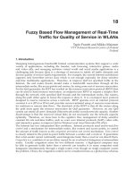
The MR fluid used for this analysis, shown in Figure 1, is mainly a dispersion of iron powder 99.9%,
as the soft magnetic material, in a carrier oil, and it was developed at ITESM, Campus Monterrey. The
iron particles size distribution has a mean value of 15.53um with standard deviation of 2.624um. The
particles are irregularly shaped and the mass fraction of the solid phase is 60%. The kind of oil used is
commercial engine oil. The total period of precipitation exceeds 40 days, without movement. The
viscosity of the MR fluid varies from 800 cP to 150,000 cP according to magnetic field applied. And,
under the influence of a magnetic field the liquid phase separates from particles after more than 24
hours.
The system used for the experiments is composed by the following components and presented
in Figure 2.The damper is aprototype made of aluminum with 0.112 m of length, 0.014 m of diameter
and 3.6 xlO"
6
m
3
of capacity. The common oil used inside the damper has been replaced with the
magnetorheological fluid, which under no current presents a similar behavior as the original fluid.
(b)
Figure 1: (a) Magnetorheological fluid and (b) prototype damper.

355
(a) (b)
Velocity effect on EDC
0.0
12000
24000
36000
0
0.0033
0.0066
0.01
Velocity (m/s)
0.5 A
3
)m/s-N( .ffeoC gnipmaD .E
A
B
Ch72-I044963.fm Page 355 Tuesday, August 1, 2006 9:53 PM
Ch72-I044963.fm Page 355 Tuesday, August 1, 2006 9:53 PM
355
A coil has been designed to be capable of produce a magnetic field of 70.8kAm"' at a current of
3ADC ,
and it was designed to be located around the damper, identified as A, in Figure 2a. A special fasten
extremity was designed to fix the upper damper part to the universal test machine, identified as B in
Figure 2a. The universal test machine used for this work is the SH1MADZU AG-1 250KN, which
allows force measurements accuracy of ± 1% of indicated test force. The module ADAMS VIEW of
MSC Software is used to create a virtual prototype of a suspension system and to view key physical
measures that emulate the data normally produced physically. An equivalent damper coefficient (EDC)
concept has been used. If the piston rod is translated at a velocity x, this will require that the fluid
trapped on one side of the piston squeeze through the spaces between the piston and the cylinder. The

fluid action opposes the motion with a magnitude given by Eqn. (1), where c is the equivalent damping
coefficient. It is equivalent because the force exerted by the damper on the mass must not deviate from
this expression no matter how fast or slow we move the mass [Cochin Ira and H.J. Plass. (1990)].
F = -ex
(1)
Velocity effect on EDC
. 36000
> 24000
O
12000
a.
0.0
•
\
^-
—000.5A
-•— 3
(a)
0.0033 0.0066
Velocity (m/s)
(b)
0.01
Figure 2: (a)Experimental set up. A; Coil and B; Fastener. And, (b) EDC behavior at different
velocities.
RESULTS
Characterization of MR Damper
Experimental Work. The characterization of the magnetorheological damper has been done to obtain
an expression, which represents its performance capabilities under different magnetic fields. Such
expression lets establish the way in which a controllable damping system can be fully used. Firstly, it
is necessary to get the set of data for the determination of force-displacement and EDC-displacement

relationship. The damper is fixed on the branches of the universal test machine; meanwhile a coil is
located around the damper body, as shown in Figure 2a. The test were done both under triangular
excitation at a constant velocity of 0.0007 m/s and at different electric current intensities through the
coil, that vary from 0.5 to 3 A. The velocity of 0.0007 m/s is selected because it represents low
velocity, high equivalent damping coefficient in addition to have a clear influence of the electrical
current, such as is shown in Figure 2b. A similar behavior has been found in reference [Yao, G.Z.
(2002)].
The relationship obtained by experiments is shown in Figure 3.
356
Mathematical Identification, 3 A
0
0.005
0.010
0.015 0.020 0.02
5
Displacement, m
0
15
20
25
30
10
5
N ,ecroF
0.030
Ch72-I044963.fm Page 356 Tuesday, August 1, 2006 9:53 PM
Ch72-I044963.fm Page 356 Tuesday, August 1, 2006 9:53 PM
356
Constitutive Model
Mathematical Identification.

The force-displacement relationship is obtained directly from the tests done, and the EDC-
displacement relationship is obtained through the use of the EDC concept using the constant velocity
of the tests and the force obtained from the following mathematical model. The constitutive model is
obtained by mathematical identification of relationships force-displacements gotten from the test.
Power equations, Eqn. (2), have been found in function of the displacement, 5, and electrical current, i.
Figure 3 and Eqn. (3), shown results for an applied current of 3 Amperes.
/ =
(2)
Where / is the force required to overcome the resistance to compress the damper. And, 8 is the
displacement given by compression in the damper.
Mathematical Identification, 3 A
0.005
0
.
01
° 0.015 0.020 0.02 0.030
Displacement, m 5
Figure 3: Mathematical identification of relationship force-displacement.
/ = 11263S
iU257
(3)
Once, all equations have been established, the constants a and b were plotted, as shown in Figure 4, to
obtain general polynomial expressions, Eqn. (4) and Eqn. (5), in function of the current.
a=-0.0079 i
2
+
1.0958
i + 8.1546
b = 0.011i
2

- 0.0209 i +0.1869
(4)
(5)
Finally, a general power equation, Eqn. (6), constituted by two polynomial expressions has been
obtained:
/=(-0.0079i
2
+1.0958i+8.1546)£'
i.Olli
2
-0.0209i I 0.1869
(6)
EDC is obtained and plotted, as Figure 5a shown, based on the constant velocity used in tests and the
force obtained from equation (6) at 0.005, 0.01, 0.015, 0.02 and 0.025 m displacements. Similar to the
previous analysis a general power equation, Eqn. (7), has been obtained:
•0.01 I; 0.0209;+O.I868
(7)
The connection between the mathematical model and the software can be given by introducing the
equivalent damping coefficient expression in function of the displacement.
357
(a)

(b)
EDC
m/s N ,.ffeoC gnipmaD .E
0
5000
10000
15000
20000

25000
30000
35000
0.00
0.01
0.02
0.03
Displacement, m
0.0 A
0.5 A
1.0 A
1.5 A
2.0
2.5
A
A
3.0 A
(a) (b)
Constant b
0.00
0.05
0.10
0.15
0.20
0.25
0.0
0. 1.0
1.5
2.0 2.5
3.0 3.5

Current , A
b eulaV
Constant a
0.
Current, A
a eulaV
12
1
8
6
4
2
0
0. 1.0 1.5 2.0 2.5 3.0
3.5
Ch72-I044963.fm Page 357 Tuesday, August 1, 2006 9:53 PM
Ch72-I044963.fm Page 357 Tuesday, August 1, 2006 9:53 PM
357
Constant a
1.5 2.0 2.5
Current, A
1.5 2.0 2.5 3.0
Current, A
(a) (b)
Figure 4: Analysis of (a) Constant a and (b) constant b.
EDC
-»-
-4-
-X-
-*-

-« -
-+"
0.0 A
0.5 A
1.0 A
1.5A
2.0 A
2.5 A
3.0A
0.00 0.01 0.02
Displacement, m
0.03
(a) (b )
Figure 5: (a) Equivalent Damping Coefficient analysis, (b) Quarter suspension car model.
Simulation of
MR Suspension
System
The use of computational software has played an important role in design. Computational techniques
are being used to complement, reinforce and specially to reduce time and money spent on experiments
and practical applications. Part one. Adjustment of the damper resistance according to constitutive
model. A quarter suspension car has been designed in ADAMSVIEW software, as shown in Figure 5b,
based on a commercial car. The analysis of the suspension was done by simulating a collision between
the car and an object at a velocity of 16.6 m/s. Once the design is completed, the damper coefficient
value was modified by introducing a set of data points, which permits the software, based on an
internal function, interpolate the discrete data. Such interpolation represents the EDC equation. Part
two.
Damper displacements at different virtual road conditions. According with the results obtained
from the comparative analysis, a strong difference behavior between passive and semi-active
suspension systems exist. The passive system shows a drastic change in the damper deformation and
chassis displacement, meanwhile the semi-active system shows an adaptive behavior according with

the respective damper displacement. When the MR damper is under a low magnetic field the
suspension system presents a smoother reaction compared with that of the passive suspension and a
higher magnetic field. According with the results obtained from the analysis, it has been demonstrated
that the equation obtained for the ECD made possible an appropriate response of the suspension
system based on the magnetic field induced. Once the behavior of the MR suspension system has been
demonstrated, a control algorithm is necessary to be developed and implemented, so that, the system
responds according to the road conditions and the comfort required by the human being.
358
Ch72-I044963.fm Page 358 Tuesday, August 1, 2006 9:53 PM
Ch72-I044963.fm Page 358 Tuesday, August 1, 2006 9:53 PM
358
CONCLUSIONS
A magnetorheological fluid has been specially developed and incorporated into a damper prototype
also specially used for this purpose. A set up with a designed load cell was used independent and also
was mounted in an Autograph Shimadzu system in order to determine the force, velocity and
displacements at different forces. The constitutive model is given by a mathematical power expression
constituted by two polynomial expressions, which are in function of the electrical current. The
suspension system is taken from a real model actually in use for a commercial automobile
characterized by its design and excellent performance. The simulated system shown the movements
and quantify the forces and displacements. The results obtained from a comparative analysis shown
strong differences between passive and semi-active suspension system. From the experiments and
simulations done, it has been shown that; the characterization of a damper can be made through of the
physical characteristics of the MR fluids, current, damper design and spring characteristics. In addition
it has been shown that the use of ADAMS software is an excellent computational tool to simulate
dynamic mechatronics systems. Finally a reconfigurable suspension system has been analyzed. Its
ability to change its rheological properties in addition to its quickly response to the circumstances
makes the MR technology a feasible way to develop other reconfigurable systems. Future work
involves the introduction of a couple systems in the simulator in order to reproduce real events for
driving, to determine the details of mechatronics control and to improve the coil's design for its
implementation in a complete prototype. A control algorithm is necessary to be developed and

implemented, so that, the system responds according to the road conditions and the comfort required
by the human being.
damper
NOMENCLATURE
a
b
c
cP
DC
EDC
8
F
Ampere
Power equation constant
Power equation exponential constant
Equivalent damping coefficient
Centipoises
Direct Current
MR Equivalent Damping Coefficient
Damper displacement or deformation
Force exerted by the damper
REFERENCES
/
i
MR
m
s
N
X
Force required to overcome

resistance
Current through the coil
Magnetorheological
Meter
Seconds
Newton
Piston rod velocity
Bossis, G. (2002). Magnetorheological Fluid. Journal of Magnetism and Magnetic Materials. 252.
224-228.
Cochin Ira and HJ. Plass. (1990). Analysis and design of dynamic systems, Harper Collins, New York,
NY.
El Wahed Ali, K. (2002). Electrorheological an Magnetorheological Fluids in Blast Resist Design
Applications. Materials & Design, 23. 391-404.
Nakamura, Taro. 2004. Variable Viscous Control Of A Homogeneous ER Fluid Device Considering
Its Dynamic Characteristics Mechatronics 14. 55-68.
Ozdalyan, B., Blundell M.V. (1998). Anti-Lock Braking System Simulation and Modeling in
ADAMS. International Conference on Simulation. 140-144.
Yao,
G.Z. (2002) MR Damper and its Application for Semi-Active Control of Vehicle Suspension
System. Mechatronics 12. 963-973.
359
Ch73-I044963.fm Page 359 Friday, July 28, 2006 1:57 PM
Ch73-I044963.fm Page 359 Friday, July 28,2006 1:57 PM
359
SOFT-SENSOR BASED TREE DIAMETER
MEASURING
Vesa Holtta
Control Engineering Laboratory, Helsinki University of Technology
P.
O. Box 5500, FI-02015 TKK, Finland

ABSTRACT
The forest harvester used for felling timber is a complex machine with a high degree of automation. To
work properly, automatic functions need accurate measurements. Tn this paper tree diameter measure-
ment is improved using different filtering and smoothing algorithms. The cases where smoothing is done
during stem processing and after the stem has been processed are treated separately. Validation using
manually measured data indicates that the methods that are presented improve the performance of the
diameter measurement considerably.
KEYWORDS
Measurement, filtering, smoothing, Kalman filtering, Kalman smoothing
INTRODUCTION
Currently the vast majority of wood felled in Finland is felled with a forest harvester. In spite of the con-
siderable amount of automation that helps the harvester operator in his work, felling timber can still be
seen as handicraft. The operator must be a trained professional who is able to navigate the harvester in
the woods without damaging the environment, and to choose the trees to cut so that future growth of the
forest is guaranteed. Achieving these goals is compromised if the operator must concentrate on too many
secondary tasks. Consequently, the need of operator interventions in less important tasks should be
minimized. This is not possible unless the operator can rely on the automatic functions.
One field where a computer can outperform a human operator is bucking, i.e. selecting the points where
the stem should be cut to logs. The price of a log is determined by its volume, but also by its grade
(stock, paper-wood, etc.). The grade can often be changed by choosing the cutting points differently.
Optimizing the bucking such that the value of the stem is maximized is a well-suited task for a com-
puter. In order for the optimization to be successful, the length and diameter measurements that are fed
to the optimization algorithm must be reliable. However, several factors can degrade the quality of the
360
Ch73-I044963.fm Page 360 Friday, July 28, 2006 1:57 PM
Ch73-I044963.fm Page 360 Friday, July 28,2006 1:57 PM
360
measurement signals during stem processing, thus resulting in non-optimal bucking. One criterion of the
grade of a log is the top diameter. If the top diameter is measured incorrectly, the log may be classified
to the wrong grade. Usually this means that a stock becomes a less valuable paper-wood log.

In addition to the optimization of bucking, accurate length and diameter measurements are needed also
for computing the volume of the logs. The volume determines the price of the log, and consequently
inaccurate measurements cause financial loss either to the seller or to the buyer of the wood. The prob-
lem is highly relevant, since measurements done by the harvester were used as the delivery measurement
for 65 % of the timber harvested in Finland in 2002. In standing sales of privately owned forests the
amount is even larger, 87 %. (Metsateho, 2003) In other countries the volume of the wood is measured
on the roadside before transportation, or at the saw mill, because the harvester measurement is not con-
sidered to be as reliable and objective as other methods. If using the harvester measurement became
widely accepted, the cost of this second measurement could be saved.
In this work a soft-sensor approach is used to improve the accuracy of the stem diameter measurement.
Using a soft-sensor means that instead of measuring a process variable directly with one physical sensor,
measurements form several sensors and other knowledge of the process are incorporated using software
to obtain an even more accurate measurement.
MECHANICAL TIMBER HARVESTING
There are different methods for mechanised timber harvesting differing by their philosophy and the ma-
chines needed. In North America the full-tree and tree-length methods are common whereas in
Scandinavia the cut-to-length method is dominant. In the cut-to-length method the trees are felled, de-
limbed and bucked (i.e. cut to logs) with a forest harvester. The harvester is equipped with measuring
devices that measure the length and diameter of the stem. Optimization algorithms choose the bucking
such that the value of the stem is maximized. Once the stems are processed, a forwarder carries the logs
to the roadside for further transportation. A cut-to-length forest harvester can be divided into four main
parts:
engine and power transmission, cabin and controls, crane and harvester head. The diesel engine is
used for rotating the supply pumps of work hydraulics and hydrostatic transmission. The supply pump of
work hydraulics delivers hydraulic power to the crane, to the harvester head and to all the auxiliary func-
tions of the machine. The hydrostatic transmission consists of a variable displacement pump, of a
variable displacement hydraulic motor and of mechanical transmission to the wheels. The cabin is
equipped with the controls that are needed for operating the functions of the harvester and with a display
module, which gives the operator information on the harvesting process and on the state of the harvester.
The most complex part of the harvester is the harvester head, which has a large-scale effect on the over-

all timber harvesting efficiency, and on the quality of the harvested timber. Its main functions are
sawing, feeding, delimbing of branches, and measuring log length and diameter profile. Trees are felled
and stems are cut to logs with a hydraulically actuated chain saw. Once sawing is complete, the stem is
fed to a new cutting point with the hydraulic feeding rollers. To prevent the feeding rollers from slip-
ping, the rollers are pressed hard against the stem with a hydraulic cylinder. In front and behind of the
feeding rollers there are delimbing knives, which wrap around the stem. As the stem is fed to the next
cutting point, branches are cut when they meet the delimbing knives. Delimbing knives also prevent the
stem from falling out of harvester head grasp during the feeding operation. The diameter of the stem is
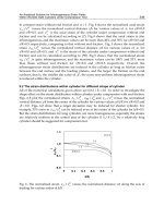
measured using the delimbing knives. The setup is depicted on the left in Figure 1 where the delimbing
knives can be seen holding the stem against the frame of the harvester head. Both delimbing knives are
fitted with a potentiometer that gives a voltage that is proportional to the position of the knife. This
measuring arrangement assumes that the stem stays in contact with the harvester head frame and that the
delimbing knives touch the surface of the stem. If these assumptions do not hold, a measurement error
will be introduced.
361
0 2 4 6 8 10 12 14 16 18 20
0
50
100
150
200
250
300
Length [m]
]mm[ retemaiD
Ch73-I044963.fm Page 361 Friday, July 28, 2006 1:57 PM
Ch73-I044963.fm Page 361 Friday, July 28,2006 1:57 PM
361
Figure 1: Correct stem position (left) and a "hanging" stem (right).
DIAMETER MEASUREMENT PROCESSING

\
S
i 10 12
Length [m]
Figure 2: Typical diameter profile of a stem. Note the level sections and the drop in diameter.
A typical diameter profile of a stem is presented in Figure 2. The diameter in millimeters is on the verti-
cal axis and the length in meters is on the horizontal axis, so that the bottom of the tree is on the left and
the top is on the right. There are two characteristic unnatural features in the diameter profiles measured
by a harvester. First, there are long level sections in the diameter profile, i.e. the diameter of the stem
seems to remain constant. Second, there are abrupt drops in the profile. Both can be seen in Figure 2.
Since the delimbing knives measure the diameter of the stem, they must follow the surface of the stem as
closely as possible. Moreover, the stem should stay at all times against the frame of the harvester head.
Loss of contact between the stem and the frame of the harvester head causes the distance between the
stem and the frame to be added to the diameter. Tf the stem loses contact with the harvester head (on the
right in Figure 1), the delimbing knives open, giving a diameter measurement that increases towards the
top of the stem. The measuring system of the harvester requires diameters to be monotonically decreas-
ing, and outputs a constant diameter value until the diameter decreases again. The result is a level
section in the diameter profile. When feeding ends and the stem stops, the delimbing knives grasp the
stem with maximum force, forcing the delimbing knives against the stem and the stem against the har-
vester head. This can be seen as the sharp narrowing in the diameter profile if the delimbing knives were
open or if the stem was not against the harvester head. Thus the measurement following a sharp narrow-
ing can be considered to be more accurate than the ones before the narrowing. Other sources of error
with less significance are e.g. branches between the harvester head frame and the stem, hysteresis in the
potentiometers that measure the position of the delimbing knives, incorrect calibration of the measuring
device, and the functioning of the diameter measurement processing algorithm in some special cases.
Different aspects must be taken into account when designing algorithms for processing the diameter
measurements to get more accurate results. Due to the large amount of disturbances that is present in the
362
Ch73-I044963.fm Page 362 Friday, July 28, 2006 1:57 PM
Ch73-I044963.fm Page 362 Friday, July 28,2006 1:57 PM

362
working environment of the harvester, any algorithm that attempts to correct the functioning of some
system in the harvester must be robust. Currently the harvester measures the diameter online while the
stem is processed without using future measurements to estimate the current diameter (filtering case).
The estimate is used whenever a diameter measurement is needed, for instance to predict the tapering of
the stem and to compute the volume of a log. In this paper three approaches for processing the meas-
urements are discussed: online filtering, online smoothing and offline smoothing.
A dataset consisting of 479 logs was used to evaluate the performance of the methods. The diameter
profile of each log in the dataset was measured manually. The measurements were taken with a measur-
ing interval of 0.3 meters at an accuracy of
1
mm. The diameter was measured along two perpendicular
lines,
and the mean of the measurements was taken to be the final value. The manual measurements
were regarded to be correct and were compared to the diameter profile measured by the harvester. The
sum of square errors at each measurement point and at the cutting points divided with the number of the
measurement points were used as metrics for the performance of the methods.
ONLINE FILTERING
First a simple linear approximation was used. The diameter measurements on the level sections of the
stem profile are rejected and estimated by fitting a linear function in least squares sense to the valid
measurements. Estimated diameters are obtained by evaluating the function at the measurement points.
A second approach was to use a Kalman filter. Kalman filters are estimators that are used for deducing
the true value of a variable in a dynamical system. If the measurements given to a Kalman filter contain
normally distributed uncorrelated noise, then the estimates are optimal with respect to all quadratic func-
tions of the estimation error. (Grewal et al., 1993) The Kalman filter needs a model of the system to
work. Tree tapering curves have been studied previously to some extent, for example polynomial models
were used by Laasasenaho (1982) and in mixed linear regression models by Lappi (1986). These ap-
proaches were not used in this study because of the relatively high complexity of the models. It can be
concluded from the abovementioned studies that the parameters of the models vary by geographic region
and by tree species, so an adaptive model is needed. The current solution is to use a tapering matrix

which is updated during harvesting, and this is the approach that was used also in this study. In this ap-
plication a first order time-variant filter was used. The tapering matrix is a model of the change of the
stem diameter between two consecutive measurements at each relative height. If the measured diameter
stays constant, the magnitude of the noise covariance is increased to account for the increased uncer-
tainty in the measurements. This results in reducing the weight that is given to the difference between
the measured and estimated diameter values when the next diameter estimate is computed. The meas-
urement noise in this application is neither normally distributed nor uncorrelated, which degrades the
optimality of the estimates. However, a Kalman filter is still worth studying because of its ability to han-
dle measurements with varying uncertainty. Kalman filtering was also applied such that the output of the
filter is used at the level sections of the stem profile. When a level section is found, the tapering rate of
the filtered profile is set to be the same as the current tapering rate obtained from the Kalman filter.
Finally, a backward approximation method was used. The method tries to fix previous measurements by
recalculating them. Each time the algorithm detects a large drop in the diameter profile it checks if there
is a level section before the drop. If this is the case, the algorithm connects the beginning of the level
section with the measurement at the bottom of the drop.
The two first filters improve the accuracy of the diameter measurement for the whole stem as well as in
the cutting points. Since the Kalman filter is based on a model of the stem profile, the results are de-
pendant of the quality of the model. Even if the model was good for the majority of the trees on a stand,
most likely some of the trees would have a very different profile due to environmental conditions, and
363
Ch73-I044963.fm Page 363 Friday, July 28, 2006 1:57 PM
Ch73-I044963.fm Page 363 Friday, July 28,2006 1:57 PM
363
their filtering result would be poor. Using Kalman filtering only at level sections of the stem profile and
backward approximation are poor solutions since they follow the original measurement too closely, im-
proving the diameter estimate only locally. Although the filtering methods give good results, because of
their lack of robustness they should not be used if smoothing methods are applicable.
ONLINE SMOOTHING
The simplest solution is to smooth the diameter profile by computing the average of the measurements
inside a window, i.e. a portion of the diameter profile containing an equal amount of measurements on

each side of the current measurement. The window is centered at the measurement that is being esti-
mated. A second approach is to fit a polynomial to the values inside the window. Like in the averaging
method, some measurements are considered before and after the current measurement. Polynomial fit-
ting may give hugely erroneous results if the number of fitting points is small compared with the order
of the polynomial. This may occur if many fitting points are removed because of level sections in the
diameter profile. The basic polynomial fitting method can be improved by assigning different weights to
different measurements. A large weight is assigned to points that are situated after large drops in the
diameter profile, which is justified by the characteristics of the measurement process. A Kalman filter
can be also used to smooth measurements. The model for the tapering of the stem and changing of the
noise were implemented like in the Kalman filter online filtering method.
Online smoothing methods are better and more robust than the online filtering methods discussed earlier,
because in smoothing it is possible to use measurements before and after the point to be estimated. Thus
smoothing should be used instead of filtering whenever possible. The simple average yields good results
both when the whole stem and when the cutting points are considered. The result is most of all due to the
fact that the averaged profiles are smooth and resemble the true stem profiles. Windowed weighted
polynomial fitting is good in the sense that it gives profiles that pass near the bottoms of large drops in
the diameter profile. Polynomial fitting suffers from the unpredictable behavior of polynomials when
there are not enough fitting points. The algorithm discards measurements that are on level sections of the
stem profile. This leads essentially to extrapolating the diameter when long level sections are encoun-
tered, fn the methods where the amount of measurements to be taken into account can be changed,
increasing the window size is advantageous, fncreasing the number of measurements improves the ro-
bustness of the algorithms and makes it possible for them to take forthcoming changes in the diameter
earlier into account. Like in filtering case, also in smoothing the quality of the results given by the Kal-
man filter depend on the quality of the stem tapering model. The better robustness of the smoothing
approach when compared with the filtering approach may compensate some flaws of the model.
OFFLINE SMOOTHING
The first algorithm that was used was linear approximation of incorrect measurements. The method
searches the first and last point of each level section. The first point is connected with a line to the point
that follows the last point of the level section and the line is used as the diameter estimate instead of the
original measurement. This method can be generalized by fitting a polynomial to all the measurements

in the least squares sense. The measurements that are situated on the level sections of the profile are not
taken into account since they can be considered erroneous.
The next method added to the previous one weighting of the points that follow large drops in the diame-
ter profile. As stated before, the points following large drops are closer to the true diameter of the stem,
because the delimbing knives have most likely been in contact with the stem at these points. In the algo-
rithm the weighting factor is decreased in order to take into account the increasing uncertainty as
measuring continues after the drop. If a level section is detected, the weight is returned to the normal
364
Ch73-I044963.fm Page 364 Friday, July 28, 2006 1:57 PM
Ch73-I044963.fm Page 364 Friday, July 28,2006 1:57 PM
364
level. This method can be changed by using weighting coefficients that depend of the size of the drop in
the diameter profile. Large drops are given a larger weight in order to get the fitted polynomial closer to
the measurements following large drops. Another adjustment to the weighted polynomial fitting method
is to change weighting according to the smoothness of the stem. This is motivated by the experimental
result that weighted polynomial fitting is good for stems containing many drops in the diameter profile,
whereas polynomial fitting is more suited for smooth stem profiles. The two improvements to the ordi-
nary weighted polynomial fitting can be used also together so that the overall weighting is determined by
the smoothness of the stem and local weighting by the size of the drops in the diameter profile.
The most significant difference is between the methods based on linear approximation and on polyno-
mial fitting. The former works locally and improves diameter accuracy only little or not at all. The
polynomial fitting methods that can utilize better the global knowledge of the diameter measurements
have a notable effect on the accuracy of diameter measuring. Offline smoothing could be advantageous
particularly considering volume determination. After the logs have been bucked, their volume is saved to
the harvester database. If the stem profile was smoothed offline before the volume is computed, accu-
racy could be better due to a more accurate diameter measurement. The methods that are based on
polynomial fitting or weighted polynomial fitting produce very smooth stem profiles. Smoothness could
be an advantage if the profiles are used to update a stem narrowing matrix or some other prediction tool.
CONCLUSIONS
Several methods were presented to improve the quality of stem diameter measurements. More reliable

automatic operations in forest harvesters help the operator to concentrate more on planning and other
tasks that cannot be done automatically. In addition to this, more accurate diameter measuring has sev-
eral advantages, like maximizing the value of the timber, making the work more efficient, and
eliminating the need of measuring the timber twice. Diameter measurement error along the whole stem
and in the cutting points can be reduced by using the measurement processing algorithms presented.
When the sum of square errors in all measurement points is considered, the improvement is with online
filtering up to 10.2 %, with online smoothing up to 15.3 %, and with offline smoothing up to 18.9 %.
When the sum of square errors in the cutting points is considered, the improvement is with online filter-
ing up to 9.8 %, with online smoothing up to 10.7 %, and with offline smoothing up to 14.1 %.
The results obtained in this paper should be applicable to all harvesters that have a measurement system
similar to the one used in this study. However, all manufacturers use their own algorithms and imple-
mentations in their machines, which may cause the methods presented in this paper to perform
differently. The compatibility of the algorithms must be verified case-by-case. Many of the methods
presented in this paper decrease the error in the diameter measurement. However, when considering the
value of the results, it must be taken into account that the dataset used to validate and compare the meth-
ods is relatively small, which decreases the reliability of the results. The methods contain also
parameters that have been adjusted according to the properties of this dataset. Further studies will be
needed to show if these parameters need to be changed for different felling sites.
REFERENCES
Grewal, Mohinder S. and Angus P. Andrews (1993). Kalman Filtering. Prentice-Hall, Inc., New Jersey.
Laasasenaho, Jouko (1982). Taper curve and volume functions for pine, spruce and birch. Finnish Forest
Research Institute, Helsinki.
Lappi, Juha (1986). Mixed linear models for analyzing and predicting stem form variation of scots pine.
The Finnish Forest Research Institute, Helsinki.
Metsateho (2003). Metsdteho website. URL: />365
Ch74-I044963.fm Page 365 Tuesday, August 1, 2006 9:45 PM
Ch74-I044963.fm Page 365 Tuesday, August 1, 2006 9:45 PM
365
STUDY ON-MACHINE WORK PIECE MEASUREMENT ON 5-AXIS
CONTROLLED MACHINING CENTER

Shunsuke Nakamura
1
Yukitoshi Ihara
2
'Major in Mechanical Engineering, Osaka Institute of Technology Graduate School,
5-16-1
Omiya, Asahi-ku 535-8585 Osaka, JAPAN
"Department of Mechanical Engineering, Osaka Institute of Technology,
5-16-1
Omiya, Asahi-ku 535-8585 Osaka, JAPAN
ABSTRACT
The study presents an application of machined work piece measurement system with the laser
displacement sensor and Cs axis control on five-axis controlled machining center. Generally,
post-process measurement of multi-face machined product is carried on a coordinate measuring
machine (CMM), however, this way cannot achieve either high productivity because of loading and
unloading of work piece nor low cost with expensive CMM. To solve this problem, On-machine work
piece measurement with the laser displacement sensor is proposed in this paper. The main objective of
this research is to establish work piece measurement system on five-axis controlled machining center
and to develop measurement software for On-machine work piece measurement, which collaborate
commercial CAD/CAD software.
KEY WORDS
On-machine measurement, five-axis controlled machining center, work piece measurement, mold
machining
INTRODUCTION
Nowadays the style design becomes increasingly important for consumer electronics and consumer
goods industries. Thus die/mold shape becomes too complicate to be machined for conventional 3-axis
machining center with high speed and high accuracy. In addition, even for industrial parts such as
automotive parts or aircraft parts, not only complex shape which 5-face machining is needed but also
high dimensional accuracy for expanded function and capacity are required. On this ground, demand
of 5-axis machining center increases rapidly, which enables to machine complex shape parts by

obtaining cutting tools' multiple degree of freedom. Generally, one axis measurement by using caliper
or micrometer is not suitable for products that are machined by 5-axis machining center because it is
too complicate to be measured all form and dimensions. Thus, in real manufacturing process,
machined products are loaded to expensive measurement-only machine such as CMM. What is more, a
large amount of time is needed for complex shape measurement even by measurement-only machine.
In this reason, total productivity is not so high although 5-axis machining center is introduced for
efficient machining. Thus, manufacturer who use 5-axis machining center is eager to get quicker and
366
Ch74-I044963.fm Page 366 Tuesday, August 1, 2006 9:45 PM
Ch74-I044963.fm Page 366 Tuesday, August 1, 2006 9:45 PM
366
higher productive manufacturing system, which enables maximum capacity of 5-axis machining
center's productivity.
Post measurement systems using some sensor and Cs control on machine tools have been developed
for confirming shape and dimension. In these systems, measurements are carried on the machine tool's
table, so work piece loading for the measurement is not required. There are two proposed measuring
sensors for On-machine work piece measurement. One is a contact triggering touch probe with a
simple mechanism called 3-D touch probe. The other is non-contact laser displacement sensor with
sophisticated electronic optical device. 3-D touch probe is commonly used in On-machine
measurement, and On-machine measurement with correcting process is already proposed [1]. However,
the proposed system is only used for dimensional measurement and not suitable for free form shape
measurement such as die/mold shape. On the other hand, laser displacement sensor has a possibility
for a free form shape because it has an ability that acquire large amount of points at high speed.
Nakagawa showed the advantage of laser displacement sensor on free curved surface measurement [2].
In this report, On-machine measurement of a mold which had free curved surfaces was carried on the
3-axis controlled machining center using laser displacement sensor. When normal vector of
measurement surface is inclined to laser, error arises. Moreover, the angle between laser and normal
vector is larger, the measurement is impossible. In this case, the measurement can be done by giving
two additional degrees of freedom to the laser displacement sensor. The additional degree of freedom
is realized by adding rotary axis of 5-axis machining center. On the 5-axis machining center, laser

always radiate perpendicularly to the measurement surface.
In this research, we try to use orientation control of the spindle in order that a laser sensor can always
direct perpendicularly to the measurement surface.
Point of measurement
error
Measuring trace
Lazer Vector
(a) Conventional method under 3Axis control (b) New method under 5Axis control
Figure 1: Measuring by conventional method and proposed method
CONCEPT OF MACHINED MEASUREMENT ON 5-AXIS CONTROL
With laser displacement sensor on 3-axis controlled machine tool, laser vector is traced as shown in
Figure 1 during measuring operations. Conventionally, On-machine work piece measurement is carried
by tracing surface in simultaneous 2-axis control on 3-axis controlled machining center. The principle
of the laser displacement sensor using this research is shown in Figure 2. Triangulation method is
adopted for the laser displacement sensor. As compared with other measuring devices, measurement
resolution of dimension is good, and measurement can apply even if measuring surface is glossy metal.
Although the sensor has the excellent feature for shape measurement, measurement error arises if laser
vector is inclined against measurement surface. And it is impossible to measure surface if laser vector
is almost parallel against measurement surface. Normally, die and mold has a steep inclination which
causes measurement error. This is a critical problem for precision shape measurement which has
3-dimentional free form such as die/mold. So, it is necessary to direct laser to the normal direction of
367
Ch74-I044963.fm Page 367 Tuesday, August 1, 2006 9:45 PM
Ch74-I044963.fm Page 367 Tuesday, August 1, 2006 9:45 PM
367
the surface
as
correctly
as
possible

for
executing surface measurement with high accuracy. Then,
as
mentioned above,
we tiy to use
additional
two
rotary axes
of
5-axis machining center
for
surface
measurement. Laser vector
is
traced
by
using orientation control
of
the spindle
on
five axis machining
center
as
shown
in
Figure
l(b).
With this method,
not
only measurement error

is
reduced
but
also
all
surface measurement
in
particular
die of
convex
is
enabled.
For
these reason, On-machine work piece
measurement
on
5-axis controlled machining center
has an
advantage
for
work piece measurement
after machining.
Circuit
of
signal amplification
Semiconductor laser
Object lens
Receive light element
Receive light lens
Work piece

J
Displacement
1 ^^f^^
Standard position
Figure
2:
Theoretical mechanism
of
laser displacement sensor
I Spindle
: Laser
| displacement
L
:
sensor
I
i
J
L- — 5axis-Machining center — — L_ —Personal computer
Figure
3:
On-machine measurement system
ON-MACHINE WORK PIECE MEASUREMENT SYSTEM
The machined work piece measurement system consists
of
5-axis controlled machining center,
commercial CAD/CAM software,
a
personal computer,
a

laser displacement sensor (includes
controller),
and
encoder counter
for PC as
shown
in
Figure
3.
Signal lines
of
linear scales
and
angle
encoders which
are
equipped
in the
machine tool
for
position feedback control
are
divided
and
connected
to the
encoder counter boards which
are
installed
in the

personal computer,
in
order
to
acquire
the
exact position information
of
5-axis machining center. Digital data
can be
outputted
and
inputted
by
Ethernet system between
PC and
5-axis machining center. RS-232C
is
used
to
obtain
measured data
by the
laser displacement sensor between
the
counter
of
the laser displacement sensor
and
PC. The

6-axis control machine tool
is
used
in the
study
as a
multi-axis machine tool made
by
MORISEIKI CO., LTD.
It
provides machining capabilities beyond
the
standard 3-axis control machine
because
of its
flexibility. Additionally,
the
machine
has C
s
axis which controls
the
rotational angle
of
the main spindle
of
the 5-axis control machine, which
has two
rotational axes,
A and C (as B)

axis
as
368
Ch74-I044963.fm Page 368 Tuesday, August 1, 2006 9:45 PM
Ch74-I044963.fm Page 368 Tuesday, August 1, 2006 9:45 PM
368
shown in Figure 4. The rotary motions around Xaxis as well as 7 axis and the Z axis are designated as
A,
C (as B) and C
|S
respectively. The inclination and rotation of the work piece is executed by A and C
axis respectively, while the C
s
axis controls laser device direction for realizing high measurement
accuracy.
Figure 4: 5-axis machining center
MEASUREMENT SOFTWARE
In this system, commercial CAD/CAM system: Pro/ENGINEER is used for modeling as well as
machining and measurement. Additionally we use versatile post processor setup application: GPOST
which is collaborated with Pro/NC. The post processor setup application can change parameters and
add a routine macro easily. Thus, we setup two post processors for simultaneous 5-axis control
machining and measurement with laser displacement sensor. On CAM section (cutter location
generation support system) generates CL data both for machining and for measurement. CL for
machining has an inclination to normal vector of a free form surface for enhanced machining
efficiency as shown in Figure 5. As opposed to it, CL for measurement may always suit normal of a
free form surface as shown in Figure 5. CAM software can easily set up parameter of the inclination
angle to the normal direction of curved surface. NC data for machining center is created by post
processor. NC data is composed of the coordinate value of cutting point and angle expression of the
tool orientation. Post processor for the measurement generates NC data for the measurement. NC data
for the measurement has some special routine macro (called 'switch motion') in order to arrange

measurement data with a personal computer easily. Carrying out pick feed, measurement is performed
so that the whole surface may be traced. Therefore, plunging operation which does not trace the
measurement surface, retraction operation, and rapid traverse positioning operation follows as an
additional operation. It is necessary to notify PC about these non-measurement times in order to hold
down consumption of a useless memory. Then, operation which notifies the switch of measurement (:
switch motion) was introduced. The switch motion is the specific motion for notifying software about
the joint of measurement by changing coordinate value. The motion consists of Z-axis movement and
dwell. Secondary, we have developed PC software for the measurement on 5-axis machining center
because both coordinate values and laser data are required in measurement with high accuracy.
Furthermore, it is necessary to convert the 3-dimensional form data of a measured model from the
acquired coordinates which include angular position of rotary table and displacement from the laser
sensor. Then we developed software with these function. The main functions of the software is as
follows; inputting CL and NC data which were generated from commercial CAM for measurement,
reading machine coordinates and laser displacement sensor value. And the software monitors start and