Microsensors, MEMS and Smart Devices - Gardner Varadhan and Awadelkarim Part 12 pps
Bạn đang xem bản rút gọn của tài liệu. Xem và tải ngay bản đầy đủ của tài liệu tại đây (2.27 MB, 30 trang )
ACOUSTIC
WAVES
313
M2
layer
(waveguiding layer
-
usually
SiO
2
)
Figure
9.8
Schematic
of a
Love wave propagation region
and
relevant layers
Figure
9.9
Wave generation
on
Love wave mode devices
The
basic principle behind
the
generation
of the
waves
is
quite similar
to
that presented
in
the
description
of an
SH-SAW sensor.
The
only difference would
be the
fact
that
the
Love wave mode would
be the
same SH-SAW mode propagating
in a
layer that
was
deposited
on top of the
IDTs.
This
layer
helps
to
propagate
and
guide
the
horizontally
polarised waves that were originally excited
by the
IDTs deposited
at the
interface between
the
guiding layer
and the
piezoelectric material beneath
(Du et al.
1996).
The
particle
displacements
of
this wave would
be
transverse
to the
wave-propagation direction, that
is,
parallel
to the
plane
of the
surface-guiding layer.
The
frequency
of
operation
is
determined
by
the IDT finger-spacing and the
shear wave velocity
in the
guiding layer. These
SAW
devices have shown considerable promise
in
their application
as
microsensors
in
liquid
media (Haueis
et al.
1994; Hoummady
et al.
1991).
In
general,
the
Love wave
is
sensitive
to the
conductivity
and
permittivity
of the
adjacent
liquid
or
solid medium (Kondoh
and
Shiokawa 1995).
The
IDTs generate waves
314
INTRODUCTION
TO SAW
DEVICES
that
are
coupled into
the
guiding layer
and
then propagate
in the
waveguide
at
angles
to
the
surface.
These
waves
reflect
between
the
waveguide (which
is
usually deposited
from
a
material whose density would
be
lower than that
of the
material underneath) surfaces
as
they travel
in the
guide above
the
IDTs.
The frequency of
operation
is
determined
by
the
thickness
of the
guide
and the IDT finger-spacing
(Tournois
and
Lardat 1969). Love
wave
devices
are
mainly used
in
liquid-sensing
and
offer
the
advantage
of
using
the
same
surface
of the
device
as the
sensing active
area.
In
this manner,
the
loading
is
directly
on
top of the
IDTs,
but the
IDTs
can be
isolated
from the
sensing medium that could,
as
stated previously, negatively
affect
the
performance
of the
device
(Du et al.
1996).
It
is
again important that interfaces (guiding layer, substrate)
be
kept undamaged
and
care
taken
to see
that
the
deposition
process
used gives
a
fairly
uniform
film at a
constant
density
over
the
thickness (Kovacs
et al.
1993).
Love wave sensors have been
put to
diverse applications, ranging
from
chemical
microsensors
for the
measurement
of the
concentration
of a
selected
chemical compound
in
a
gaseous
or
liquid environment (Kovacs
et al.
1993; Haueis
et al.
1994; Gizeli
et al.
1995)
to the
measurement
of
protein composition
of
biologic
fluids
(Kovacs
et al.
1993;
Kovacs
and
Venema 1992; Grate
et al.
1993a,b). Polymer (e.g. PMMA)
layer-based
Love wave sensors
(Du et al.
1996)
are
used
to
assess
experimentally
the
surface mass-
sensitivity
of the
adsorption
of
certain proteins
from
chemical compounds.
It has
also
been shown recently that
a
properly designed Love wave sensor
is
very promising
for
(bio)chemical sensing
in
gases
and
liquids because
of its
high sensitivity (relative change
of
oscillation
frequency
due to a
mass-loading); some
of the
sensors
with
the
aforemen-
tioned characteristics have already been
realised
(Kovacs
et al.
1993).
As is
discussed
in
the
next chapter,
the
main advantage
of
shear Love modes applied
to
chemical-sensing
in
liquids
derives
from the
horizontal polarisation,
so
that they have
no
elastic interactions
with
an
ideal liquid.
It is
also sometimes noticed that viscous
liquid
loading causes
a
small
frequency-shift
that increases
the
insertion loss
of the
device
(Du et al.
1996).
9.5
CONCLUDING REMARKS
This
chapter should provide
the
reader with
the
necessary background
to the
basic prin-
ciples governing waves
and SAW
devices
7
.
Figure 9.10 summarises
the
different
types
of
waves that
can
propagate through
a
medium.
These
are
waves that travel through
the
bulk
of the
material (Figure 9.10
(a)
and
(b)).
The
compressive
(P)
wave
is
sometimes called
a
longitudinal wave
and is
well
known
for the way in
which sound travels through air.
On the
other hand,
the S
wave
is a
transverse
bulk wave
and
looks
like
a
wave traveling down
a
piece
of
string.
In
contrast,
waves
can
travel along
the
surface
of a
media, (Figure 9.10
(c) and
(d)).
These
waves
are
named
after
the
people
who
discovered them.
The
Rayleigh wave
is a
transverse wave that
travels along
the
surface
and the
classic example
is the ripples
created
on the
surface
of
water
by a
boat moving along.
The
Love wave
is
again
a
surface wave,
but
this time
the
waves
are SH or
vertical. This mode
of
oscillation
is not
supported
in
gases
and
liquids,
and
so
produces
a
poor coupling constant. However, this phenomenon
can be
used
to a
great advantage
in
sensor applications
in
which
poor
coupling
to air
results
in low
loss
(high Q-factor)
and
hence
a
resonant device with
a low
power consumption.
7
Some
of the
material
presented
here
may
also
be
found
in
Gangadharan
(1999).
CONCLUDING
REMARKS
315
Figure
9.10 Pictorial representation
of
different
waves
From these fundamental properties
of
waves,
it
should
be
noted that
for
applications
considered here, such
as
ice-detection, there
are a
variety
of
possible options. Because
ice-detection primarily involves sensing
the
presence
of a
liquid (e.g. water),
it is
obvious
that Rayleigh wave modes
and flexural
plate
(S)
modes cannot
be
used because
of
their
attenuative characteristics. Therefore,
it is
imperative that only those wave modes
are
used
whose
longitudinal component
is
small
or
negligible compared with
its
surface-parallel
316
INTRODUCTION
TO SAW
DEVICES
Table
9.2
Structures
of
Love, Rayleigh SAW, SH-SAW, SH-APM
and FPW
devices
and
compar-
ison
of
their operation
Device
type
Love
SAW
Rayleigh
SAW
SH-SAW SH-APM
FPW
Substrate
Typical
frequency
(MHz)
ST-quartz ST-quartz LiTaO
3
ST-quartz Si
x
N
y
/ZnO
95-130
80-1000
90-150
160 1-6
Ua
U
b
t
Media
Transverse
Parallel
Ice to
liquid
chemosensors
Transverse
parallel
Normal
Strain
Transverse Transverse Transverse
parallel
Parallel Parallel Normal
Gas
liquid
Gas
liquid
Gas
liquid
chemosensors
a
U is the
particle
displacement
relative
to
wave
propagation
b
U
t
is the
transverse
component
relative
to
sensing
surface
components.
For
this reason, either
a
Love
SAW or an SH
wave-based
APM
device
could
be
used. However, because
the
ratio
of the
volume
of the
guiding layer
to the
total
energy
density
is the
largest
for a
Love wave device,
it is
natural
to
choose
a
Love wave
device
for the
higher sensitivity toward
any
perturbation
at the
liquid
interface.
Finally, Table
9.2
summarises
the
different
types
of SAW
devices described
in
this
chapter.
This
reference table
also
gives
the
typical operating frequencies
of the
devices,
along with
the
wave mode
and
application area.
REFERENCES
Atashbar,
M. Z.
(1999).
Development
and
fabrication
of
surface acoustic wave
(SAW)
oxygen
sensors
based
on
nanosized TiO2 thin
film, PhD
thesis, RMIT, Australia.
Avramov,
I. D.
(1989). Analysis
and
design
aspects
of
SAW-delay-line-stabilized oscillators,
Pro-
ceedings
of the
Second International
Conference
on
Frequency Synthesis
and
Control, London,
April
10-13,
pp.
36-40.
Bechmann,
R.,
Ballato,
A. D. and
Lukaszek,
T. J.
(1962). "Higher order temperature coefficients
of the
elastic stiffnesses
and
compliances
of
alpha-quartz," Proc.
IRE,
p.
1812.
Cambell,
C.
(1989).
Surface
Acoustic
Wave
Devices
and
their Signal Processing Applications,
Academic
Press,
London,
p.
470.
Campbell,
C.
(1998).
Surface
Acoustic
Wave
Devices
and
their Signal Processing Applications,
Academic
Press,
London.
d'Amico,
A. and
Verona,
E.
(1989).
"SAW sensors,"
Sensors
and
Actuators,
17,
55–66.
Du,
J. et al.
(1996).
"A
study
of
love wave acoustic
sensors,"
Sensors
and
Actuators
A, 56,
211–219.
REFERENCES
317
Ewing,
W. M.,
Jardetsky, W.S.,
and
Press,
F.
(1957). Elastic
Waves
in
Layered Media, McGraw-
Hill,
New
York.
Gangadharan,
S.
(1999).
Design, development
and
fabrication
of a
conformal love wave
ice
sensor,
MS
thesis (Advisor V.K. Varadan), Pennsylvania State University, USA.
Gizeli,
E.,
Goddard,
N. J.,
Lowe,
C. R. and
Stevenson,
A. C.
(1992).
"A
love plate biosensor
util-
ising
a
polymer
layer,"
Sensors
and
Actuators
A, 6,
131–137.
Gizeli,
E.,
Liley,
M. and
Lowe,
C. R.
(1995).
Detection
of
supported lipid layers
by
utilising
the
acoustic love waveguide device: applications
to
biosensing, Technical Digest
of
Transducers '95,
vol.
2,
IEEE,
pp.
521-523.
Grate,
J. W.,
Martin,
S. J. and
White,
R. M.
(1993a). "Acoustic wave microsensors, Part
I,"
Analyt-
ical
Chem.,
65,
940-948.
Grate,
J. W.,
Martin,
S. J. and
White,
R. W.
(1993b).
"Acoustic
wave
microsensors.
Part II,"
Analytical Chem.,
65,
987-996.
Haueis,
R. et al,
(1994).
A
love wave based oscillator
for
sensing
in fluids,
Proceedings
of
the 5th
International Meeting
of
Chemical Sensors (Rome, Italy),
1,
126–129.
Hoummady,
M.,
Hauden,
D. and
Bastien,
F.
(1991).
"Shear
horizontal wave sensors
for
analysis
of
physical
parameters
of
liquids
and
their mixtures," Proc.
IEEE
Ultrasonics Symp.,
1,
303-306.
Kondoh,
J. and
Shiokawa,
S.
(1995). Liquid identification using SH-SAW sensors, Technical Digest
of
Transducers'95, vol.
2,
IEEE,
pp.
716-719.
Kondoh,
J.,
Matsui,
Y. and
Shiokawa,
S.
(1993). "New biosensor using shear horizontal surface
acoustic wave device," Jpn.
J.
Appl. Phys.,
32,
2376-2379.
Kovacs,
G. and
Venema,
A.
(1992).
"Theoretical
comparison
of
sensitivities
of
acoustic shear wave
modes
for
(bio)chemical
sensing
in
liquids,"
Appl. Phys.
Lett.,
61,
639–641.
Kovacs,
G.,
Vellekoop,
M. J.,
Lubking,
G. W. and
Venema,
A.
(1993).
A
love wave sensor
for
(bio)chemical sensing
in
liquids, Proceedings
of
the 7th
International
Conference
on
Solid-State
Sensors
and
Actuators,
Yokohama, Japan,
pp.
510-513.
Love,
A. E. H.
(1934).
Theory
of
Elasticity, Cambridge University Press, England.
Mason,
W. P.
(1942). Electromechanical Transducers
and
Wave
Filters,
Van
Nostrand,
New
York.
Morgan,
D. P.
(1978).
Surface-Wave
Devices
for
Signal Processing, Elsevier,
The
Netherlands.
Nakamura,
N.,
Kazumi,
M. and
Shimizu,
H.
(1977). "SH-type
and
Rayleigh-type surface waves
on
rotated Y-cut
LiTaO3,"
Proc. IEEE Ultrasonics Symp.,
2,
819-822.
Shiokawa,
S. and
Moriizumi,
T.
(1987). Design
of SAW
sensor
in
liquid,
Proceedings
of the 8th
Symposium
on
Ultrasonic Electronics,
July,
Tokyo.
Smith,
W. R.
(1976).
"Basics
of the SAW
interdigital
transducer,"
Wave
Electronics,
2,
25–63.
Tournois,
P. and
Lardat,
C.
(1969).
"Love
wave dispersive delay lines
for
wide band pulse compres-
sion," Trans. Sonics Ultrasonics, SU-16, 107–117.
Varadan,
V. K. and
Varadan,
V. V.
(1997). "IDT,
SAW and
MEMS sensors
for
measuring deflec-
tion,
acceleration
and ice
detection
of
aircraft," SP1E,
3046,
209-219.
Viktorov,
I. A.
(1967). Rayleigh
and
Lamb
Waves:
Physical
Theory
and
Applications, Plenum Press,
New
York.
White,
R. W. and
Voltmer,
F. W.
(1965). "Direct piezoelectric coupling
to
surface elastic waves,"
Appl.
Phys.
Lett.,
7,
314–316.
This page intentionally left blank
10
Surface Acoustic Waves
in
Solids
10.1 INTRODUCTION
Acoustics
is the
study
of
sound
or the
time-varying deformations,
or
vibrations,
in a
gas,
liquid,
or
solid.
Some nonconducting crystalline materials become electrically
polarised
when they
are
strained.
A
basic
explanation
is
that
the
atoms
in the
crystal lattice
are
displaced when
it is
placed under
an
external load. This
microscopic
displacement produces electrical dipoles
within
the
crystal and,
in
some materials, these dipole moments combine
to
give
an
average
macroscopic moment
or
electrical
polarisation. This phenomenon
is
approximately linear
and
is
known
as the
direct piezoelectric (PE)
effect
(Auld 1973a).
The
direct
PE
effect
is
always accompanied
by the
inverse
PE
effect
in
which
the
same material will become
strained
when
it is
placed
in an
external electric
field.
A
basic understanding
of the
generation
and
propagation
of
acoustic waves (sound)
in
PE
media
is
needed
to
understand
the
theory
of
surface acoustic wave (SAW) sensors.
Unfortunately,
most textbooks
on
acoustic wave propagation contain advanced mathe-
matics (Auld 1973a)
and
that makes
it
harder
to
comprehend. Therefore,
in
this chapter,
we
set out the
basic underlying principles that describe
the
general problem
of
acoustic
wave
propagation
in
solids
and
derive
the
basic equations required
to
describe
the
prop-
agation
of
SAWs.
The
different
ways
of
representing acoustic wave propagation
are
outlined
in
Sec-
tions
10.2
and
10.3.
The
concepts behind stress
and
strain over
an
elastic continuum
are
discussed
in
Section 10.4, along with
the
general equations
and
concepts
of the
piezoelectric
effect.
These equations together with
the
quasi-static approximation
of the
electromagnetic
field are
solved
in
Section 10.5
in
order
to
derive
the
generalised
expres-
sions
for
acoustic wave propagation
in a PE
solid.
The
boundary conditions that restrict
the
propagation
of
acoustic waves
to a
semi-infinite solid
are
included,
and the
general solu-
tion
for a SAW is
presented.
An
overview
of the
displacement modes
in
Love, Rayleigh,
and
SH-SAW waves
are finally
presented
in
Section 10.5. Consequently, this chapter
is
only
intended
to
serve
as an
introduction
to the
displacement modes
of
Love, Rayleigh,
and SH
waves.
The
components
of
displacements have been shown only
for an
isotropic elastic solid.
The
equations
for the
complex reciprocity
and the
assumptions used
to
derive
the
pertur-
bation
theory
are
elaborated
in
Appendix
I.
More
advanced
readers
may
wish
to
omit this chapter
or
refer
to
specialised text-
books
published elsewhere (Love 1934; Ewing
et al.
1957; Viktorov 1967;
Auld
1973a,b;
320
SURFACE
ACOUSTIC
WAVES
IN
SOLIDS
Slobodnik 1976). This chapter
on the
basic understanding
of
wave theory, together
with
the
next chapter
on
measurement theory, should provide
all
readers
with
the
neces-
sary background
to
understand
the
application
of
interdigital transducer (IDT) microsen-
sors
and
microelectromechanical system (MEMS) devices presented later
in
Chapters
13
and 14.
10.2 ACOUSTIC
WAVE
PROPAGATION
The
most general type
of
acoustic wave
is the
plane wave that propagates
in an
infinite
homogeneous medium.
As
briefly
summarised
at the end of
Chapter
9 for
those readers
omitting
that chapter, there
are two
types
of
plane waves, longitudinal
and
shear waves,
depending
on the
polarisation
and
direction
of
propagation
of the
vibrating atoms within
the
medium
(Auld
1973a). Figure 10.1 shows
the
particle displacement
profiles
for
these
two
types
of
plane waves
1
.
For
longitudinal waves,
the
particles vibrate
in the
propaga-
tion
direction (y-direction
in
Figure 10.1 (a)), whereas
for
shear waves, they vibrate
in a
plane normal
to the
direction
of
propagation, that
is, the x- and
z-directions
as
seen
in
Figure 10.1(b)
and
(c).
When boundary restrictions
are
placed
on the
propagation medium,
it is no
longer
an
infinite
medium,
and the
nature
of the
waves changes.
Different
types
of
acoustic waves
may
be
supported
within
a
bounded medium,
as the
equations given below demonstrate.
Surface
Acoustic
Waves
(SAWs)
are of
great interest here;
in
these waves,
the
traveling
Figure
10.1
Particle
displacement profiles
for (a)
longitudinal,
and
(b,c)
shear
uniform
plane
waves. Particle propagation
is in the
y-direction
1
Also
see
Figure
9.10
in
Chapter
9 on the
introduction
to SAW
devices.
INTRODUCTION
TO
ACOUSTICS
321
y-polarized
x-polarized
z-polarized
x-propa
z-polarized
x-polarized
y-polarized
Figure
10.2
Acoustic
shear
waves
in a
cubic
crystal
medium
wave
is
guided along
the
surface with
its
amplitude decaying exponentially away
from
the
surface
into
the
medium. Surface waves were introduced
in the
last chapter
and
include
the
Love
wave
mode,
which
is
important
for one
class
of IDT
microsensor.
10.3
ACOUSTIC
WAVE
PROPAGATION
REPRESENTATION
Before
a
more detailed analysis
of the
propagation
of
uniform plane waves
in
piezoelectric
materials
in the
following sections,
a
pictorial representation
of the
concept
of
shear wave
propagation
is
presented. Figure 10.2 illustrates shear wave propagation
in an
arbitrary
cubic crystal medium.
An
acoustic wave
can be
described
in
terms
of
both
its
propagation
and
polarisation directions. With reference
to the X, Y, Z (x, y, z)
coordinate system,
propagating SAWs
are
associated with
a
corresponding polarisation,
as
illustrated
in the
figure.
10.4
INTRODUCTION
TO
ACOUSTICS
10.4.1
Particle Displacement
and
Strain
As
stated
earlier,
acoustics
is the
study
of the
time-varying deformations
or
vibrations
within
a
given material medium.
In a
solid,
an
acoustic wave
is the
result
of a
deformation
of
the
material.
The
deformation occurs when atoms within
the
material move
from
their
equilibrium positions, resulting
in
internal restoring forces that return
the
material back
to
equilibrium (Auld 1973a).
If we
assume that
the
deformation
is
time-variant, then
322
SURFACE
ACOUSTIC
WAVES
IN
SOLIDS
Figure
10.3
Equilibrium
and
deformed
states
of
particles
in a
solid
body
these restoring forces together with
the
inertia
of the
particles result
in the net
effect
of
propagating wave motion, where each atom oscillates about
its
equilibrium point.
Generally,
the
material
is
described
as
being elastic
and the
associated
waves
are
called
elastic
or
acoustic waves. Figure 10.3 shows
the
equilibrium
and
deformed states
of
particles
in an
arbitrary solid body
- the
equilibrium state
is
shown
by the
solid dots
and
the
deformed state
is
shown
by the
circles.
Each particle
is
assigned
an
equilibrium vector
x and a
corresponding displaced position
vector
y (x, t),
which
is
time-variant
and is a
function
of x.
These continuous position
vectors
can now be
related
to find the
displacement
of the
particle
at x
(the equilibrium
state) through
the
expression
u(x,
t)
=y(x,
t)—
x
(10.1)
Hence,
the
particle vector-displacement
field
u(x,t)
is a
continuous variable that
describes
the
vibrational motion
of all
particles within
a
medium.
The
deformation
or
strain
of the
material occurs only when particles
of a
medium
are
displaced relative
to
each other. When particles
of a
certain body maintain their relative
positions,
as is the
case
for rigid
translations
and
rotations
2
, there
is no
deformation
of the
material. However,
as a
measure
of
material deformation,
we
refer
back
to
Figure 10.3
and
extend
the
analysis
to
include
two
particles,
A and B,
that
lie on the
position vector
x
and
x + dx,
respectively.
The
relationship that describes
the
deformation
of the
particles
2
Only
at
constant velocity because acceleration induces strain.
INTRODUCTION
TO
ACOUSTICS
323
between these
two
points
after
a
force
has
been applied
may be
written
as
(x,f)
=
2S
ij
(x, t)dx
i
dx
j
(10.3)
where
S
ij
(x,
t) is the
second-order strain tensor
3
defined
by
±
+
3u
i
+
9j±^-\
(]04)
Cy
dXi dX{ dXj J
with
the
subscripts
of i, j, and k
being
x, y, or z.
For rigid
materials,
the
deformation gradient expressed
in
Equation (10.4) must
be
kept small
to
avoid permanent damage
to the
structure; hence,
the
last term
in the
above
expression
is
assumed
to be
negligible,
and so the
expression
for the
strain-displacement
tensor
is
rewritten
as
du
t
(x,t)
2
j(x,t)-]
4
-
dxt
J
t
, , ,
Sij(x,
0
=
-
—
-
h
-4 -
(10.5)
10.4.2 Stress
When
a
body vibrates acoustically, elastic restoring forces,
or
stresses, develop between
neighbouring particles.
For a
body that
is
freely
vibrating, these forces
are the
only ones
present. However,
if the
vibration
is
caused
by the
influence
of
external forces,
two
types
of
excitation forces
(body
and
surface
forces)
must
be
considered. Body forces
affect
the
particles
in the
interior
of the
body directly, whereas surface forces
are
applied
to
material
boundaries
to
generate acoustic vibration.
In the
latter case,
the
applied excitation does
not
directly
influence
the
particles within
the
body
but it is
rather transmitted
to
them through
elastic restoring forces,
or
stresses, acting between neighbouring particles.
Stresses
within
a
vibrating medium
are
defined
by
taking
the
material particles
to be
volume elements,
with
reference
to
some orthogonal coordinate system (Auld 1973a).
In
order
to
obtain
a
clearer
understanding
of
stress,
we
make
the use of the
following simple example.
Let us
assume
a
small surface area
AA on an
arbitrary solid body with
a
unit normal
n,
which
is
subjected
to a
surface force
AF
with uniform components AF
i
.
The
surface
AA may be
expressed
as a
function
of its
surface components
AA
j
and the
unit normal components
n
j
as
follows:
A
j
=n
j
AA (10.6)
with
the
subscript
j
taking
a
value
of 1, 2, or 3.
The
stress tensor, T
ij
,
is
then related
to the
surface force
and the
surface area through
AF
i
with
the
subscripts
i and j
taking
a
value
of 1, 2, or 3.
3
A
tensor
is a
matrix
in
which
the
elements
are
vectors.
324
SURFACE
ACOUSTIC
WAVES
IN
SOLIDS
Moreover,
if we
consider
the
stress
tensor T
ij
to
be
time-dependent
and
acting upon
a
unit
cube (assumed
free
body),
the
stress analysis
may be
extended
to
deduce
the
dynamical equations
of
motion through
the sum of the
acting forces. Thus,
= p-
dt
2
(10.8)
where
p is the
mass density,
F
i
are the
forces acting
on the
body
per
unit
mass,
and u
i
,
represents
the
components
of
particle displacements along
the
i-direction.
10.4.3
The
Piezoelectric Effect
Within
a
solid medium,
the
mechanical forces
are
described
by the
components
of the
stress
field
T
ij
,
whereas
the
mechanical deformations
are
described
by the
components
of
the
strain
field
S
ij
.
For
small static deformations
of
nonpiezoelectric elastic solids,
the
mechanical stress
and
strain
fields are
related according
to
Hooke's
Law
(Slobodnik
1976):
Tij=c
ijk
,S
k
,
(10.9)
where
T
ij
are the
mechanical stress second-rank tensor components (units
of
N/m
2
),
S
kl
are the
strain second-rank tensor components (dimensionless),
and
c
ikl
is the
elastic
stiffness
constant (N/m
2
) represented
by a
fourth-rank tensor. Taking into account
the
symmetry
of the
tensors,
the
previous equation
can be
reduced
to a
matrix equation using
a
single
suffix.
Thus,
the
tensor components
of T, S, and c are
reduced according
to the
following
scheme
of
replacement
(Auld
1973a; Slobodnik 1976):
(32)
=
(23)
(22)
2;
(13)
=
(31)
(33)
3 5;
(21)
=
(10.10)
Therefore,
the
elastic
stiffness
constant
can be
reduced
to a 6 x 6
matrix. Depending
on
the
crystal symmetry, these
36
constants
can be
reduced
to a
maximum
of 21
independent
constants.
For
example, quartz
and
lithium
niobate, which present trigonal symmetry,
have
their number
of
independent constants reduced
to
just
6
(Auld
1973b):
c
u
C\2
C\2
C\4
0
C
12
c\\
C
13
—C
14
0
0
C\2
C\3
C
33
0
0
0
C\4
—C
14
0
C44
0
0
0
0
0
0
C44
C\4
0
0
0
0
C
11
–C
12
))
(10.11)
In
piezoelectric materials,
the
relation given
by
Equation (10.8)
no
longer holds true.
Coupling between
the
electrical
and
mechanical parameters gives
rise to
mechanical
deformation
and
vice versa
upon
the
application
of an
electric
field. The
mechanical
stress relationship
is
thus
extended
to
– e
kij
E
k
(10.12)
ACOUSTIC
WAVE PROPAGATION
325
where
e
kij
is the
piezoelectric constant
in
units
of
C/m
2
,
E
k
is the kth
component
of the
electric
field, and
c
E
ijkl
is
measured either under
a
zero
or a
constant electric
field.
In
nonpiezoelectric materials,
the
electrical displacement
D is
related
to the
electric
field
applied
by
D=s
r
e
0
E
(10.13)
where
e
r
is the
relative permittivity, formerly
called
the
dielectric constant,
and e
0
is the
permittivity
of
vacuum,
now
known
as the
electric constant.
For
piezoelectric materials,
the
electrical displacement
is
extended
to:
Di
=
e
ikl
S
kl
+e
S
ik
E
k
(10.14)
where
e
S
ik
is
measured
at
constant
or
zero strain.
Equations (10.12)
and
(10.14)
are
often
referred
to as
piezoelectric constitutive
equations.
In
matrix notation, Equations (10.12)
and
(10.14)
can be
written
as
(Auld
1973b):
[T]
=
[c][S]–[e
T
]E
D
=
[e][S
] +
[e]E (10.15)
where,
[e] is a 3 x 6
matrix with
its
elements depending
on the
symmetry
of the
piezo-
electric crystal
and
[e
T
]
is the
transpose
of the
matrix [e].
For
quartz having
a
trigonal
crystal
classification,
the [e]
matrices
are
/ e
{[
-e
n
0 e\4 0 0 \
[e]
= 0 0 0 0
-e
14
-e
11
(10.16)
V
0 000 0 0
The
difference between
poled
and
naturally
piezoelectric
materials
is
that
in the
former,
the
presence
of a
large number
of
grain boundaries
and its
anisotropic nature would lead
to a
loss
of
acoustic signal
fidelity at
high frequencies. This
is one of the
reasons
SAW
devices are,
usually,
only fabricated
out of
single-crystal piezoelectrics.
10.5
ACOUSTIC
WAVE
PROPAGATION
10.5.1
Uniform
Plane
Waves
in a
Piezoelectric
Solid:
Quasi-Static
Approximation
For the
numerical calculations
of
acoustic wave propagation,
the
starting point
is the
equation
of
motion
in a
piezoelectric material
(Auld
1973a)
pu
i
=
T
ij.j
i, j =
1,2,
3
(10.17)
where,
p is the
mass density,
and u
i
is the
particle displacement.
In
tensor notation,
the two
dots over
a
symbol denotes a
2
/at
2
and a
subscript
i
preceded
by a
comma denotes a/ax
i
.
The
piezoelectric constitutive equations
in
(10.15)
are
rewritten
in
tensor notation:
326
SURFACE ACOUSTIC WAVES
IN
SOLIDS
+
eE
kk
(10.18)
(10.19)
with
i, j, k, and /
taking
the
values
of 1, 2, or 3.
The
strain-mechanical displacement relation
is:
The
absence
of
intrinsic charge
in the
materials
is
assumed; therefore,
Dj.j=0
(10.20)
(10.21)
The
quasi-static approximation
is
valid because
the
wavelength
of the
elastic waves
is
much
smaller than that
of the
electromagnetic waves,
and the
magnetic
effects
generated
by
the
electric
field can be
neglected
(Auld
1973a):
E
k
=
-<f>.k
(10.22)
where
</>
is the
electric potential associated
with
the
acoustic wave.
The
problem
of
acoustic wave propagation
is
fully
described
in
Equations (10.17)
to
(10.22). These equations
can be
reduced through substitution
to
*i —
c
jkl
u
l.jk
0 =
ejki
-
efkbjk
(10.23)
(10.24)
The
geometry
for the
problem
of SAW
wave propagation
is
shown
in
Figure 10.4.
It has
a
traction-free surface
(x
3
= 0)
separating
an
infinitely
deep solid
from the free
space.
The
traction-free boundary conditions
are
(Viktorov 1967; Varadan
and
Varadan 1999)
r,-
3
=0 for x
3
= 0
(10.25)
where
i
takes
a
value
of 1, 2, or 3.
The
solutions
of the
coupled wave Equations (10.23)
and
(10.24) must satisfy
the
mechanical boundary conditions
of
Equation (10.25).
The
solutions
of
interest here
are
Figure
10.4
Coordinate
system
for SAW
waves
showing
the
propagation
vector
ACOUSTIC
WAVE
PROPAGATION
327
SAWs
that propagate parallel
to the
surface with
a
phase velocity
uR and
whose displace-
ment
and
potential amplitudes decay with distance away
from
the
surface
(X
3
,
> 0). The
direction
of
propagation
can be
taken
as the
x
1
-axis,
and the
(x
1
,
x
3
)
plane
can be
defined
as
the
sagittal plane.
Note that
the
propagation geometry axes depicted
in
Figure 10.4
do not
always corre-
spond
to the
axes
in
which
the
material property tensors
are
expressed. There
are
transfor-
mation formulae that
can be
applied
to the
property tensors
so
that
all the
above equations
hold
for the new
axes.
The
elastic constants
(Q/M),
the
piezoelectric constants
(e,-^/),
and
the
dielectric constants
(e,-
7
)
can be
substituted
by
c'
ijkl
, e'
ijkl
, s'^.
The
primed parameters
refer
to a
rotated coordinate system through
the
Euler transformation matrix (Auld 1973a).
The
solutions
for
Equations (10.23)
and
(10.24) have
the
form
of
running waves:
the
surface
wave solution
is in the
form
of a
linear combination
of
partial waves
of the
form
(Auld
1973a)
ui
= Ai
exp(—kx
3
)
exp
-jco
\t-~\\
(10.26)
(p
— B
exp(— kxj)
exp
—jco
I t - I and x > 0
(10.27)
L
V VR / J
Here,
co is the
angular frequency
of the
electrical signal,
k is the
wave number, given
by
27T/A,,
and A. is the
wavelength, given
by
2nvR/co.
When
the
three particle displacement components exist,
the
solutions
are
called gener-
alised
Rayleigh waves.
The
crystal symmetry
and
additional
boundary conditions
(elec-
trical
and
mechanical) impose
further
constraints
on the
partial wave solutions.
If the
sagittal plane
is a
plane-of-mirror symmetry
of the
crystal,
x\ is a
pure-mode axis
for
the
surface wave, which involves only
the
potential
and the
sagittal-plane components
of
displacement.
Because
the
Rayleigh wave
has no
variation
in the
X2
-direction,
the
displacement
vectors have
no
component
in the x
2
-direction
and the
solution
is
given
as
follows
(Varadan
and
Varadan 1999):
Assume displacements
u\ and u3 to be of the
form
A
exp(— bx
3
)
exp[jk(x
1
—
ct)]
and
B
exp(—
bxT,} exp[jk(x
1
—
ct)],
and u
2
equal
to
zero, where
the
elastic half-space that
exists
for x
3
is
less than
or
equal
to
zero,
B and A are
unknown amplitudes,
k is the
wave
number
for
propagation along
the
boundary (x
1
-axis)
and c is the
phase velocity
of
the
wave.
Physical
consideration
requires
that
b
can,
in
general,
be
complex with
a
positive real part. Substitution
of the
assumed displacement into
Navier—
Stokes equation
gives
(Varadan
and
Varadan 1999)
V-T-/t)
= 0
(10.28)
and
use of the
generalised
Hooke's
law for an
isotropic elastic solid yields
two
homoge-
neous
equations
in A and B. For a
nontrivial solution,
the
determinant
of the
coefficient
matrix
vanishes, giving
two
roots
for b in
terms
of the
longitudinal
and
transverse veloc-
ities. Substitution
of the
roots
of b
obtained,
as
shown earlier, into
the
homogeneous
equations
in A and B
gives
the
amplitude ratios. Thus,
we
obtain
the
general displacement
solution
(Equation 10.28) (Varadan
and
Varadan 1999).
328
SURFACE
ACOUSTIC
WAVES
IN
SOLIDS
Unstressed
Rayleigh
wave
Figure
10.5 Particle displacement
on the
sagittal plane
for the
Rayleigh wave
These
displacements
are as
shown
in
Figure 10.5.
It is
seen that
as u$ is in
phase
quadrature with
MI,
the
motion
of
each particle
is an
ellipse. Because
of the
change
in
sign
in u
1
at a
depth
of
about
0.2
wavelengths,
the
ellipse
is
described
in
different
directions above
and
below this point.
At the
surface,
the
motion
is
retrograde, whereas
lower down
it is
prograde.
u
1
=
[A
1
exp(-£i.*3)
+
A
2
exp(-b
2
*3)]exp[jk:(.xi
-
x
1
)]
"3
= (-
-
ct)] (10.29)
where
b
1
= k(1 -
c
2
/v
2
)1/2
and
b
2
= k(1 -
c
2
/v
2
)
1/2
The
longitudinal
and
transverse velocities,
v
1
and v,, are
given
by
where
the
Lames'
constants
G is
given
by
E
m
/2(l
+ v) and A is
given
by
vE
m
/[(l
+ v)
(1 —
2v)] with
v
being
Poisson's
ratio
and E
m
being Young's modulus.
10.5.2
Shear Horizontal
or
Acoustic Plate Modes
Acoustic plate
modes
(APW)
or
shear horizontal (SH) waves
in a
half-space utilise single-
crystal quartz substrates. These
act as an
acoustic waveguide
by
confining
the
acoustic
energy between
the
upper
and
lower surfaces
of the
plate. Such
a
mechanism
is
used
to
confine
waves traveling between
an
input
and
output IDT.
SH
modes
may be
thought
of
as
those waves with
a
superposition
of SH
plane waves,
which
are
multiply
reflected
at
some angle between
the
upper
and
lower surfaces
of the
quartz plate. These upper
and
lower faces impose
a
transverse resonance condition, which results
in
each
SH
mode
having
the
displacement maxima
at the
surfaces,
with
sinusoidal variation between
the
surfaces.
The
solution
is
simply
a
plane
shear
wave propagating
parallel
to the
surface, with
its
amplitude
independent
of
X3,
within
the
material.
The
phase velocity
is
equal
to v,. The
particle displacement associated with
the nth
order
SH
plate mode (propagating
in the
ACOUSTIC
WAVE
PROPAGATION
329
x\-direction)
has
only
an
x2-component
and is
given
by the
following equation (see
Auld
1973a,b):
u
2
=
wo
cos —
I
x
2
+ - J
exp[j
(cat
-
p
n
x\)] (10.30)
where
b is the
plate thickness,
u
2
is the
particle displacement
at the
surface,
n is the
transverse modal index (0,1,2,3 ),
and t is
time.
The
exponential term
in the
equation
describes
the
propagation
of the
displacement
profile down
the
length
of the
waveguide
(along
the x
1
-direction) with angular
frequency
w and
wave number
B
n
given
by
(10.31)
where
VQ
is the
unperturbed propagation velocity
of the
lowest-order mode.
The
cross-sectional displacement profiles
(in the x
2
—
x
3
plane)
for the
four
lowest-
order isotropic
SH
plate modes
are
shown
in
Figure 10.6.
It is
also noticed that each
mode
has
equal displacements
on
both sides
of the
acoustic plate mode (APM) sensor,
allowing
the use of
either side
for
sensing measurements.
Figure
10.6 Displacement modes
for (n = 0, 1, 2, 3)
SH-APM
modes
(z::x
1
,
x
2
:
y::x
3
)
330
SURFACE ACOUSTIC WAVES
IN
SOLIDS
10.5.3
Love
Modes
Ewing
and
co-workers (1957) were
one of the first to
point
out
from
long-period
seismo-
graphs that
in
addition
to
measuring
the
characteristic horizontal motion during
the
main
disturbance
of the
earthquake,
the
seismographs
also
showed
a
large amount
of
transverse
components.
This
early established
fact
in
seismology
was
explained
in
1911
by
Love,
and
he
easily showed that there could
be no SH
surface wave
on the
free
surface
of a
homogeneous elastic half-space (Love 1934). Hence, this simple model could
not
explain
the
measurements. Love, however, showed subsequently that
the
waves involved were
SH
waves,
confined
to a
superficial
layer
of an
elastic half-space
and the
layer
having
a
different
set of
properties
from
the
rest
of the
half-space. Following
Love's
treatment
here, Love waves
can be
considered
as
SAWs that propagate along
a
waveguide made
of
a
layer
of a
given material
M
2
(e.g. glass) deposited
on a
substrate made
of
another
material
M
1
,
(e.g. stable temperature (ST)-cut quartz),
with
different
acoustic properties
and,
effectively,
an
infinite
thickness when compared
with
the
original layer.
These waves
are
transverse
and
they bring only shear
stresses
into action.
The
displace-
ment
vector
of the
volume element
is
perpendicular
to the
propagation direction O-x
1
and
is
oriented
in the
direction
of the
O-x
2
axis. Because
the
Love wave
is a
surface wave,
the
propagating energy
is
located
in the
layer
and in
that part
of the
substrate that
is
close
to
the
interface.
Its
amplitude decreases exponentially
with
depth. However,
it
should also
be
noted that materials should have appropriate properties
to
propagate
and
carry
a
Love
wave,
as
shall
be
discussed
in the
section hereby.
10.5.3.1
Existence conditions
of
Love waves
dispersion
equation
The
case
in
which
the two
propagating media
are
isotropic
is
examined
first. The
coor-
dinate origin
is
chosen
on the
interface;
the
O-x
1
axis
is
oriented
in the
direction
of
propagation
and the
jcs-axis
is
oriented vertically upwards (see Figure 10.7).
The
plane
SiO,
ST cut
quartz
v.
Shear
velocity
in
substrate
Direction
of
propagation
v
3
Shear
velocity
in
waveguide
Region
of
propagation
of
Love
waves
M
2
layer
Figure
10.7
Structure
of a
Love
waveguide:
M
1
is the
substrate;
M
2
is the
guiding
layer
ACOUSTIC WAVE PROPAGATION
331
Figure 10.8 Schematic
of
Love wave device used
for
calculations
x
3
= h
represents
the
free
boundary
of the
layer.
Let us
assume that displacements
are
oriented along
the
x
2
-axis
and are
independent
of x
1
.
Then,
let us
consider
a
monochro-
matic progressive wave
of
frequency
a>
propagating along
the
x
1
-axis.
Using
the
symbols
p
1
, G
1
, u
1
and P
2
, G
2
, and u
2
for the
density,
the
shear modulus
and
the
displacement vector
of the
volume elements
for the
substrate
and the
layer,
respectively;
VT\ and k\
(equal
to
CO/VTI),
the
phase velocity
of the
transverse waves
and the
wave number
in
medium
M
1
; and vj2 and k
2
(<v/VT2),
the
same quantities
in
medium A/2,
let us
finally
call
c and k
(equal
to
cafe)
the
phase velocity
and the
wave
number
of the
Love wave, whose existence
is
postulated (see Figure 10.8).
The
solutions
of the
propagation's
Equation
(10.29)
can now be
written
in the
following
way
(Varadan
and
Varadan 1999):
jkx\
u
2x2
= (B
1
+ B
2
) exp
(jcot
-
jkx
1
+
a
2
x
3
)
(10.32)
where
-
c
2
/4i
<*2
= -k\ -
c
2
/v
2
T2
(10.33)
It
can be
verified that
the
above
equation satisfies
the
Naviers Equation
(10.28)
in the
two
media
and
further
that
u
3
->• 0 as x
3
->
—
oo
(Varadan
and
Varadan 1999).
u
T1
and
V
T2
are the
transverse wave velocities,
as
defined
earlier
by
Equation (10.28).
The
three constants
A, B
1
, and B
2
are
determined
by the
boundary conditions that
require
not
only that
the
tangential stresses
0
23
cancel
out in the
plane
X
3
,
= h but
also
that they
are
continuous
as
well
as the
displacements u
1x2
and
u
2x2
in the
plane
Jt3 = 0
(Ewing
et al.
1957; Slobodnik 1976).
332
SURFACE
ACOUSTIC
WAVES
IN
SOLIDS
The first of
these conditions leads
to
B
1
exp
(—a
2
h)
- B
2
exp
(+a
2
h)
= 0
(10.34)
and
the two
other conditions lead
to A = B\ + B
2
and
a
1
G
1
A = a
2
G
2
(B
1
— B
2
)
(10.35)
This
system
of
three linear equations
has a
solution
different
from
zero (Tournois
and
Lardat
1969)
if
G
1
a
1
tan(a
2
h =
—
—
-
(10.36)
The
roots
of
this equation have
a
real value when
k
1
< k < k
2
,
that
is,
when
c
2
< c < c\.
Therefore,
a
necessary condition
of
existence
of
Love waves
is
that
the
propagation
velocity
of
transverse waves
in the
layer must
be
smaller than
the
propagation velocity
of
the
transverse waves
in the
substrate.
It
is
easy
to
deduce
from
Equation (10.36) that there
are
infinite
modes owing
to the
periodicity
of the
tangential
function;
when
c
tends
to c
1
,
tan(a
2
h)
tends toward
the
value
of
nn
(with
n
being
0, 1, 2, . . .), and for the first
mode,
the
wavelength becomes
infinite
compared with
the
thickness.
The
particle displacements occurring during
the
propagation
of
Love waves
are
easily
obtained
from Equation
(10.35).
"1x2
= A
COS[(X
2
(h
-
X
3
)]
,,ni-n
u
2x2
=
A
-
-
-
exp[y(wf
-
kx\)] (10.37)
cos a2 n
where
A is a
propagation
constant determined
by the
excitation
signal.
The
equations
in (
10.37) show that
the
displacement amplitude u
1x2
decreases
exponen-
tially
in the
substrate.
It
also
shows
that
the
different
modes
u
2x2
correspond
to 0,
1,2,
nodal planes
in the
layer. Figure 10.9(a) gives
the
shape
of
particle displacements
in the
layer
and the
substrate
for the first
three modes.
The
displacement amplitude also depends
on the
frequency,
and
Figure 10.9(b) shows
its
variation
for the first
mode. Therefore,
it
could
be
noticed that
the
energy
is
entirely
located
in the
substrate
for
very
low
frequencies
and
that
the
Love wave propagates
at
a
velocity
c\ as if the
layer
does
not
exist.
Its
thickness
is, in
fact,
negligible when
compared with
the
wavelength. Conversely,
the
acoustic energy
is
concentrated
in the
layer
for
very high frequencies,
and the
phase velocity
of the
Love waves tends toward
c
2
, the
wavelength being very small with respect
to the
thickness
of the
layer. Between these
two
limits,
the
energy progressively transfers
from
the
substrate
to the
layer, whereas
the
phase
velocity
varies
between
c\ and c
2
(Tournois
and
Lardat
1969).
Having
obtained
the
nature
of the
displacement
and the
similarity between
the
SH-SAW
waves
and
Love
modes,
we can
derive
an
expression
for the
change
in the
velocity
and
frequency
shift
for a
Love wave device using perturbation theory.
The
derivation
for
the
frequency
shift
and the
corresponding change
in
velocity have been presented
in
Appendix
I
using
the
basic equations derived
in
this chapter.
ACOUSTIC
WAVE
PROPAGATION
333
I
mode
II
mode
Particle displacement
for the first
three Love modes
+ 1
T
III
mode
Frequency
variation
of the
particle displacement
for the
first
three modes
Figure
10.9 Displacement modes
for
Love wave devices (note that
z
corresponds
to x
2
and y
corresponds
to
X
3
,
in
Figure 10.8)
10.5.3.2
Discussions
of the
characteristics
of the
Love waveguiding
materials
It
may be
noticed
from
earlier
discussions, that
the two
most important parts
of a
Love
wave sensor
are the
overlayer material
and the
piezoelectric
substrate.
Our
discussion
now
focuses
on the
salient points
of the
waveguide, particularly with respect
to the
properties
of
the
material.
Love waves propagate near
the
surface
of a
suitable substrate material when
the
surface
is
overlaid
by a
thin
film
with appropriate properties
for a
guiding layer.
An
essential condition
for the
propagation
of a
Love wave
is
that
the
shear velocity
in
the
film is
less
than that
in the
substrate. Sensitivity
to
mass-loading
is
enhanced
by
the
low
density
of the film as
well
as a
large difference between
the
shear velocities.
For a
particular guiding-layer material,
an
optimum layer thickness exists, which results
in
maximum acoustic energy density close
to the
surface
and
maximum sensitivity
to
mass-loading.
Love wave devices incorporating guiding layers
of
poly(methyl methacrylate) (PMMA)
and
sputtered SiO
2
overlaid
on
single-crystal quartz have been successfully demon-
strated
(Du et al.
1996). PMMA
has a
density
of
about 1.18 kg/m
3
and has a
shear
acoustic velocity
of
1100
m/s
(Kovacs
et al.
1993; Jakoby
and
Vellekoop 1998;
Du et al.
1996), whereas sputtered silicon dioxide
has a
density
of
about
2.3
kg/m
3
and a
shear
334
SURFACE ACOUSTIC
WAVES
IN
SOLIDS
acoustic velocity
4
of
2850
m/s
(Auld 1973a). Gizeli
and
coworkers (1995) utilised PMMA
layers
of
thickness
up to 5.6 |im
spun onto Y-cut quartz with IDTs
of
periodicity
of
45 um at the
quartz-PMMA
interface.
A
network analyser
was
used
to
monitor
the
phase
of the
wave.
The
maximum thickness reported
by
Gizeli
and
coworkers (1995)
(~1.6
um) is
considerably less than
the
estimated optimum thickness
of
approximately
3 urn of
PMMA (Shiokawa
and
Moriizumi
1988).
Kovacs
and
co-workers
(1993)
have
utilised sputtered silicon dioxide
on
ST-cut quartz. Acoustic
losses
in
SiO
2
are low
when
compared with polymers such
as
PMMA. SiO
2
is
more resistant
to
most chemicals and,
when
sputtered under optimal conditions,
has
excellent wear resistance. Because
of
tech-
nical reasons,
it was
reported that
the
maximum thickness
of
SiO
2
that
was
utilised
was
5.46
urn -
considerably less than
the
optimum value
of
approximately
6 um
(for devices
of
wavelength
40
um).
Another criterion
for the
choice
of a
suitable waveguiding material would
be the
absorption coefficient.
It
essentially
depends
on the
material structure, which
can be
poly-
crystalline, crystalline,
or
amorphous.
In
polycrystalline materials, when
the
wavelength
becomes comparable
to the
grain size because
of the
phenomenon
of
Rayleigh scattering
(Rayleigh
1924),
the
energy absorption
increases
proportionally
to
frequency
to the
fourth
power (Tournois
and
Lardat 1969).
At
higher frequencies,
it is
obvious that
the
materials
employed will have
to be
without loss-inducing grain boundaries, that
is,
either single-
crystalline
or
amorphous. Amorphous bodies, such
as
certain
glasses
and
fused
silica,
will
allow propagation with
a
limited absorption
at
frequencies
much
higher than
100
MHz.
10.6
CONCLUDING
REMARKS
In
this chapter,
the
basic equations that
describe
the
propagation
of
different
types
of
waves
in an
elastic solid have been presented
and
expressions
for the
displacement
of
particles
therein
5
have
also
been obtained.
The
emphasis
has
been
directed
toward
the
fundamental
differences between
the
Rayleigh
and SH
modes
and SH of
vibration.
The SH
and
Love wave modes have been examined
from
the
point
of
view
of
waveguide structure,
that
is, the
nature
of the
overlayer
and the
substrate. This mathematical discourse should
help readers
to
understand
the
nature
and
application
of SAW
microsensors
and
MEMS
devices
in
other
chapters.
REFERENCES
Auld,
B. A.
(1973a).
Acoustic
Fields
and
Waves
in
Solids
/,
John
Wiley
and
Sons,
New
York.
Auld,
B. A.
(1973b).
Acoustic
Fields
and
Waves
in
Solids
//,
John
Wiley
and
Sons,
New
York.
Du,
J. et al.
(1996).
"A
study
of
Love
wave
acoustic
sensors,"
Sensors
and
Actuators
A, 56,
211-219.
Ewing,
W. M.,
Jardetsky,
W. S., and
Press,
F.
(1957).
Elastic
Waves
in
Layered
Media,
McGraw-
Hill,
New
York.
Gangadharan,
S.
(1999).
Design,
development
and
fabrication
of a
conformal
love
wave
ice
sensor,
MS
thesis,
Pennsylvania
State
University,
USA.
4
This
value
is
sensitive
to the
deposition
conditions.
5
Some
of the
material
presented
here
may
also
be
found
in
Gangadharan
(1999).
REFERENCES
335
Gizeli,
E.,
Liley,
M. and
Lowe,
C. R.
(1995). Detection
of
supported lipid layers
by
utilizing
the
acoustic Love waveguide device: application
to
bioengineering, Technical Digest
of
Transducers
'95,
pp.
521–523.
Jakoby,
B. and
Vellekoop,
M. J.
(1998).
"Analysis
and
optimisation
of
Love wave
sensors,"
IEEE
Trans.
Ultrasonics,
Ferroelectrics
and
Frequency control,
45,
1293–1302.
Kovacs,
G.,
Vellekoop,
M. J.,
Lubking,
G. W. and
Venema,
A.
(1993).
A
Love wave sensor
for
(bio)chemical sensing
in
liquids, Sensors
and
Actuators,
43,
38-43.
Love,
A. E. H.
(1934).
Theory
of
Elasticity, Cambridge University Press, England.
Rayleigh,
R.
(1924).
Theory
of
Sound, Macmillan,
New
York.
Shiokawa,
S. and
Moriizumi,
T.
(1988). Design
of SAW
sensor
in
liquid, Proc.
of 8th
Symp.
on
Ultrasonic
Electronics, Tokyo,
pp.
142-144.
Slobodnik,
A. J.
(1976). "Surface acoustic waves
and
materials," Proc. IEEE,
64,
581-595.
Tournois,
P. and
Lardat,
C.
(1969).
"Love
wave dispersive delay lines
for
wide band pulse compres-
sion,"
Trans.
Sonics Ultrasonics, SU-16, 107–117.
Varadan,
V. V. and
Varadan,
V. K.
(1999).
Elastic wave propagation
and
scattering, Engineering
Science
and
Mechanics, Pennsylvania State University,
USA.
Viktorov,
I. A.
(1967). Rayleigh
and
Lamb
Waves:
Physical
Theory
and
Applications, Plenum Press,
New
York.
This page intentionally left blank
11
IDT
Microsensor Parameter
Measurement
11.1
INTRODUCTION
TO IDT SAW
SENSOR
INSTRUMENTATION
There
is no
specific design procedure
for
interdigital transducer (IDT) microsensors based
on
surface acoustic wave (SAW) delay lines. Although substantial work
has
been done
on
delay line designs
for filtering and
signal-processing applications,
the
requirements
for
SAW-based devices
are
essentially
different
from
those
for
commercial non-SAW
oscillator-based sensors (Avramov 1989).
The SAW
device should
not
only have
the
appropriate frequency-transfer characteristics,
but its
physical dimensions should also
allow
for
miniaturisation
and
remote-sensing
of a
variety
of
physical
and
chemical media.
This
chapter deals with
the
instrumentation
and
measurement
aspects
of a
typical
IDT-SAW
sensor during
the
course
of its
operation
and so
covers
the
different
measure-
ment
techniques available
and
makes
a
comparison between them.
Specifically,
Section 11.3
describes
the
basic
principles
of a
'network analyser,' whereas
subsequent
sections describe
its use to
measure
the
amplitude (Section 11.4), phase
(Section
11.5),
and
frequency (Section 11.6)
of
signals. Finally,
a
brief overview
of a
network
analyser system
is
given with particular emphasis
on the
topics
of
forward-
matching,
reverse-matching,
and
transmission (see Gangadharan 1999).
11.2
ACOUSTIC
WAVE
SENSOR
INSTRUMENTATION
11.2.1
Introduction
Acoustic
wave sensors convert
the
physical
or
chemical property
of
interest into
a
signal
suitable
for
measurement. Ultimately,
the
measured
sensor
data
must
be
processed
so
that
they
can be
presented
to the
user
in
both
a
sensible
and
meaningful
way.
The
role
of
system
instrumentation
is to
implement this task.
Ever
since
the
early work
by
Sauerbrey
and
King (Avramov 1989),
and
many
of
those that have followed,
the
vast majority
of
acoustic-sensing applications
has
involved
acoustic
sensors being used
as the
active frequency-control elements
in
oscillator circuits.
The
oscillator
output
frequency
is
then used
as the
(desired) measured parameter. This
is