Microsensors, MEMS and Smart Devices - Gardner Varadhan and Awadelkarim Part 15 pps
Bạn đang xem bản rút gọn của tài liệu. Xem và tải ngay bản đầy đủ của tài liệu tại đây (2.85 MB, 30 trang )
TESTING
OF A
MEMS-IDT
ACCELEROMETER
403
of
the
microsensor (Section
14.4.1–14.4.4).
Then
we
will discuss
the
incorporation
of a
seismic
mass
to
produce
an
inertial accelerometer (Section 14.4.5).
14.4.1 Measurement Setup
The
vector network analyser
and
associated calibration techniques make
it
possible
to
measure accurately
the
reflection
and
transmission parameters
of
devices under test
3
.
The
basic arrangement
of
such
a
measurement system
is
illustrated
in
Figure 14.4.
The
network
analyser system consists
of a
synthesized sweeper
(10
MHz–20 GHz),
the
test
set
(40
MHz-40
GHz),
HP
8510B network analyzer,
and a
display
processor.
The
sweeper
provides
the
stimulus
and the
test
set
provides
the
signal
separation.
The
front
panel
of
the
HP
8510B
is
used
to
define
and
conduct various measurements.
The
various other
instruments
are
also controlled
by the
network analyser through
the
system bus.
The
device
to be
tested
is
connected between
the
test Port
1 and
Port
2. The
point
at
which
Synthesizer sweeper
0.01
– 40 GHz
A
V
HP
8510B
Network
analyzer
Test
set
0.045
-
40
GHz
Port 1
Power Macintosh
6100/66
A
JL
A
V
HP
plotter
Apple
laser
printer
Port
2
Coaxial
cable
Coaxial
cable
Sample
holder
with
SAW
device
Figure 14.4 Basic arrangement
of the
measurement system
for the SAW
device
3
A
detailed
explanation
of SAW
parameters
and
their
measurement
is
given
in
Chapter
11.
404
MEMS-IDT
MICROSENSORS
1
V
c
^
2
r-
s
u
>
_
^
^
r >
^
^
k
S
22
—
^
Figure
14.5
Signal
flow in a
two-port
network
the
device
is
connected
to the
test
set is
called
the
reference
plane.
All
measurements
are
made with reference
to
this plane.
The
measurements
are
expressed
in
terms
of
scattering
parameters referred
to as 5
parameters. These describe
the
signal
flow
(Figure 14.5)
within
the
network.
5
parameters
are
defined
as
ratios
and are
represented
by
Sin/out,
where
the
subscripts
in
and out
represent
the
input
and
output
signals, respectively. Figure 14.5 shows
the
energy
flow in a
two-port network.
It can be
shown that
b
1
=
a
1
S
11
+
a
2
S
12
and b
2
=
a
1
S
21
+
a
2
S
22
(14.1)
and, therefore,
S
11
=
b
1
/a
1
,
S
21
=
b
2
/a
1
when
a
2
= 0; S
12
=
b
1
/a
2
,
S
22
=
b
2
/a
2
when
a
1
= 0.
(14.2)
where
S
11
and S
21
(S
12
and
S
22
)
are the
reflection
and
transmission
coefficients
for
Port 1(2), respectively.
14.4.2
Calibration Procedure
Calibration
of any
measurement system
is
essential
in
order
to
improve
the
accuracy
of
the
system. However, accuracy
is
reduced because errors, which
may be
random
or
systematic, exist
in all
types
of
measurements. Systematic
errors
are the
most significant
source
of
measurement uncertainty. These errors
are
repeatable
and can be
measured
by
the
network analyser. Correction terms
can
then
be
computed
from
these measurements.
This process
is
known
as
calibration. Random errors
are not
repeatable
and are
caused
by
variations
due to
noise, temperature,
and
other environmental factors
that
surround
the
measurement
system.
A
series
of
known standards
are
connected
to the
system
during
calibration.
The
system-
atic effects
are
determined
as the
difference between
the
measured
and the
known
response
of
the
standards. These errors
can be
mathematically related
by
solving
the
signal-flow
graph.
The
frequency
response
is the
vector
sum of all
test setup variations
in
magni-
tude
and
phase with
frequency.
This
is
inclusive
of
signal-separation devices, test cables,
and
adapters.
The
mathematical process
of
removing systematic errors
is
called error
correction.
Ideally,
with
perfectly known standards, these errors should
be
completely
characterised.
The
measurement system
is
calibrated
using
the
full
two-port calibration
TESTING
OF A
MEMS-IDT
ACCELEROMETER
405
method.
Four standard methods
are
used, namely,
shielded
open circuit, short circuit, load,
and
through. This method provides
full
correction
for
directivity, source match, reflec-
tion
and
transmission signal path
frequency
response, load match,
and
isolation
for
S
11
,
S
12
, S
21
,
and
S
22
.
The
procedure
involves taking reflection, transmission,
and
isolation
measurements.
For the
reflection measurements (S
11
, S
22
),
the
open, short,
and
load standards
are
connected
to
each port
in
turn
and the
frequency
response
is
measured.
These
six
measure-
ments
result
in the
calculation
of the
reflection error coefficients
for
both
the
ports.
For the
transmission
measurements,
the two
ports
are
connected
and the
following measurements
are
conducted: forward transmission through (S
21
-frequency
response), forward match
through
(S
21
-load), reverse transmission through
(S
12
-frequency
response)
and
reverse
match
through (S
12
-load).
The
transmission error
coefficients
are
computed
from
these
four
measurements. Loads were connected
to the two
ports
and S
21
noise
floor and S
12
noise
floor
levels were measured. From these measurements,
the
forward
and
reverse
isolation
error
coefficients
are
computed.
The
calibration
is
saved
in the
memory
of the
network
analyser
and the
correction
function
is
turned
on to
correct systematic errors that
may
occur.
14.4.3 Time Domain Measurement
The
relationship between
the
frequency domain response
and the
time domain response
is
given
by the
Fourier transform,
and the
response
may be
completely specified
in
either domain.
The
network analyser performs measurements
in the
frequency domain
and
then computes
the
inverse Fourier transform
to
give
the
time domain response. This
computation
technique
benefits
from
the
wide dynamic range
and the
error correction
of
the
frequency
domain data.
In
the
time domain,
the
horizontal axis represents
the
propagation delay through
the
device.
In
transmission measurements,
the
plot displayed
is the
actual one-way travel time
of
the
impulse, whereas
for
reflection measurements
the
horizontal axis shows
the
two-way
travel
time
of the
impulse.
The
acoustic propagation length
is
obtained
by
multiplying
the
time
by the
speed
of the
acoustic wave
in the
medium.
The
peak value
of the
time domain
response represents
an
average reflection
or
transmission over
the
frequency range.
The
time band
pass
mode
of the
network analyser
is
used
for
time
domain
analysis.
It
allows
any
frequency domain response
to be
transformed
to the
time domain.
The
Hewlett
Packard (HP) 8510B network analyser
has a
time domain feature called windowing, which
is
designed
to
enhance time domain measurements. Because
of the
limited bandwidth
of
the
measurement system,
the
transformation
to the
time domain
is
represented
by a
sin(x)/x stimulus rather than
the
ideal stimulus.
For
time band pass measurements,
the
frequency
domain response
has two
cutoff
points
f
start
and
f
stop
.
Therefore,
in the
time
band
pass mode,
the
windowing
function
rolls
off
both
the
lower
end and the
higher
end
of the
frequency
domain response.
The
minimum window option should
be
used
to
minimise
the filtering
applied
to the
frequency domain data.
Because
the
measurements
in the
frequency domain
are not
continuous but, apart
from
Af (in
Hz),
are
taken
at
discrete
frequency
points, each time domain response
is
repeated
every
1/Af seconds.
The
amount
of
time
defines
the
range
of the
measurement. Time
domain
response resolution
is
defined
as the
ability
to
resolve
two
close responses.
The
406
MEMS-IDT
MICROSENSORS
response
resolution
for the
time band pass,
using
the
minimum window,
can be
expressed
as
a
parameter
r:
1.2
r
= -—
(14.3)
f
span
where
the
frequency span
f
span
is
expressed
in Hz.
Thus,
if a frequency
span
of 10 MHz
is
used,
the
measurement system will
not be
able
to
distinguish between equal magnitude
responses separated
by
less than 0.12
us for
transmission measurements.
Time domain range
response
is the
ability
to
locate
a
single
response
in
time. Range
resolution
is
related
to the
digital resolution
of the
time domain display, which uses
the
same number
of
points
as
that
of the frequency
domain.
The
range resolution
can be
computed
directly
from the
time span
and the
number
of
points
selected.
If a
time span
of
5 us and 201
points
are
used,
the
marker
can
read
the
location
of the
response
with
a
range resolution
of
24.8
ns (5
us/201).
The
resolution
can be
improved
by
using
more
points
in the
same time span.
14.4.4
Experimental
We
now
evaluate
the
suitability
of
using
S
11
measurement
for the
measurement
of
reflec-
tions
in SAW
delay line.
The
operating principle
of the
device
is
based
on the
perturbation
in the
velocity
of the
acoustic wave
due to the
changes
in the
electrical boundary conditions.
The two
extreme
electrical
boundary conditions were applied
in
turn.
An
attempt
was
then made
to
detect
these
in
various measurement
options
that
are
available
in the
vector network analyser.
These electrical conditions represent
the
maximum change possible
for the
device designed
and
hence
are
useful
in
evaluating suitability
of any
measurement technique.
The
details
of
this device
are
given
in the
following paragraph. Split
finger
electrodes
were used
in
order
to
reduce reflections
from the
electrodes:
•
Number
of finger
pairs
is 10
•
Propagation path length
is
6944
urn
•
Operating frequency
is
82.91
MHz
Two
devices representing
the two
extreme
electrical
boundary conditions were used:
1.
A SAW
delay line with split
finger
IDTs
and
with
an
aluminum layer
in the
propagation
path.
This device represents
the
electrical boundary condition
in
which
the
electric
field
is
shorted
on the
substrate surface.
2. A SAW
delay line with split
finger
IDTs
and
without
an
aluminum layer
in the
prop-
agation path. This device represents
the
electrical boundary condition
in
which
the
electric
field
decays
at an
infinite
distance
from the
substrate surface.
Both
these
devices
have
a
propagation path length
of
6944
urn.
The SAW
propagation
velocity
on the
substrate
is
3980
m/s and the
crystal size
is (10 x 10)
mm
2
.
The
equipment
TESTING
OF A
MEMS-IDT
ACCELEROMETER
407
Figure
14.6
Measurement
of the S
11
parameter
used
for the
measurement
was an HP
Network Analyzer Model No.8753A operating
in
the
range
300 kHz to 3
GHz.
The two
ports
are
calibrated using test standards
in the
method described earlier.
The
devices
are
connected
in
turn
and the
reflection
coefficient
(S
11
)
was
measured (see
Figure
14.6).
In the S
11
measurement,
the
wave propagates
from
one set of
IDTs
to the
other
set of
IDTs
and the
reflections
due to the
second
set are
measured
at the first
set.
It
was
also
found
that
in the
linear magnitude format,
the
reflection peak
was
more
sharply
defined than
the one in the log
magnitude format.
The
measurements were trans-
formed
into
the
time domain
as the
interpretation
of the
observations
are
much
easier.
The
gating
function
of the
network analyser
was
used
to filter out the
electromagnetic
feed
through.
It
also allows appropriate scaling
of the
desired signal.
In
the
case
of the
device
with
aluminum between
the
IDTs,
the first
reflection
from
the
IDT
occurred
at
3.799
us. The
next peak beyond 3.799
us is the
reflection
from
the
crystal
edge.
For the
device without aluminum,
a
reflection
was
measured
at
3.535
us. It can be
seen that
for the
same distance traveled,
the
wave velocity
is
greater
in the
case
of the
device
without aluminum.
The
time
difference
between these
two
measurements (3.535
us
and
3.799
us) is a
measure
of the
coupling
efficiency
of the
substrate
as
well
as
mass
loading because
of the
aluminum layer between
the
IDTs.
The
theoretical calculations
for
this substrate leads
us to
expect
the
velocity
of the
wave
to
slow down
by 136 m/s
because
of the
change
in the
electrical
boundary conditions.
The
observed slowing down
of
the
wave
was
around
281
m/s. This
difference
is
probably
due to the
mass loading
effects
of the
aluminum.
The
results
of
these experiments indicate that
the
effect
of an
aluminum conductor
placed
close
to the
surface should
be
seen
in the
region between 3.535
us and
3.799
us
in
the
time domain measurement
of
S
11
.
The
experimental validation
of the
design
and the
concept
was
done
in
stages.
The first
step
in
this process
was to
conduct
an
experiment
to
qualitatively examine
the
effect
of
a
conductor close
to the
surface
and to
devise
a
measurement method.
The
three samples
used
for the
experiment
are
described here:
1.
For the
gross
or
qualitative evaluation
of the
effect,
it is
sufficient
to
place
a
conductor
close
to the
surface.
Three
samples were prepared
for
this experiment.
The
sample
consisted
of a
micromachined silicon trough
in
which aluminum
was
deposited.
The
408
MEMS-IDT
MICROSENSORS
Figure
14.7
Measurement
of the (Sj
2)
parameter
trough
is 1 \im
deep.
Within this trough,
600 nm of
aluminum
was
deposited.
This
device allows
the
conductor
to be
placed
400 nm
from
the
substrate.
2.
This
sample
is the
same
as the one
discussed
earlier,
except
that there
is a
silicon
dioxide layer
1 um
thick
on the
substrate. This sample allows
the
conductor
to be
placed
1.4 um
from
the
substrate.
3. The
third sample
is
similar
to the first
sample.
It
consists
of a
micromachined trough
that
is 1 um
deep. Silicon
is to
serve
as a
conductor. This sample
can be
used
to
evaluate
the
suitability
of
silicon
as a
conductor
for
this application.
These
samples
are
shown
in
Figure 14.8.
These
samples
are flipped
over
and are
placed
on
the
substrate. They rest
on
spacers.
The
spacers
lie
outside
the
propagation path
of the
Rayleigh wave.
The
trough
was big
enough such that when
it was
placed
on the
substrate,
it
still
left
the
substrate mechanically
free.
This
can be
easily tested
by
doing
the S\2
measurement (Figure 14.7).
These
observations were carried
out in
both
the
frequency
and
the
time domain.
The
following conclusions have been derived
from
the set of
experiments mentioned
previously.
The
arrangement
of the
spacer performs adequately
in the
placing
of the
conductor within
one
wavelength
of the
surface. Silicon instead
of
aluminum
could
be
used
for
this device.
For
this application,
it can
almost
be
considered
to be a
conductor.
The
perturbation
in the
velocity
of the
wave
is too
small
to be
measured
as a
shift
in the
amplitude response
in
both
frequency
and
time domain
with
the
given resolution
of the
network analyser.
14.4.5
Fabrication
of
Seismic
Mass
Following
the
aforementioned evaluation
of the
performance
of the IDT
microsensor,
we
will
now
discuss
the
addition
of a
seismic
mass
to the
wafer
to
produce
an
accelerometer.
The
fabrication
of a
seismic mass
is a two
mask
process.
Here,
the
masks were designed
for
the
process
using
the
commercial
software
package
of
L-Edit (Tanner
Tools
Inc.).
A
TESTING
OF A
MEMS-IDT
ACCELEROMETER
409
Oxide
500 nm
p
-
type
silicon
wafer
a.
Oxidation
p-type
silicon
wafer
c.
Pattern
and
develop photoresist
p-type
silicon
wafer
e.
Strip oxide
to
complete
spacer
fabrication
Photoresist
p-type
silicon
wafer
b.
Spin
on
photoresist
p-type
silicon
wafer
d.
Plasma
etch
Si to get
required
spacer
height
Spacer
100
nm,400
nm,
1
(im,
2
|o,m
f.
Perspective
view
of
device
after
first
stage
of
fabrication
Figure
14.8
Basic
steps
in the
fabrication
of the
spacers
4"
silicon wafer
was
chosen
and
four
different
wafers were processed,
as
each spacer
height requires
a
separate
wafer.
The first
step
in the
fabrication process
was the
creation
of the
spacer
of the
desired
height.
The
next step
is the
fabrication
of the
reflector arrays.
These
two
stages
are
described with
the
help
of
Figures 14.8
and
14.9.
The
basic steps
in the
process involve
the
growth
and
patterning
of an
oxide mask, followed
by dry
etching
of
silicon
by
plasma.
The
steps required
to
fabricate
the
spacers
are as
follows:
Four p-type
wafers
of
silicon (100)
of
resistivity between
2 and 5
ohm.cm were used.
1.
A 500 nm
thick silicon dioxide
is
grown. This oxide layer will
act as a
mask
for the
dry
etching (Figure 14.8(a)).
2.
Photoresist
is
spun
on the
oxide layer (Figure 14.8(b)).
The
resist
is
baked
to
improve
adhesion.
3. The first
mask
is
aligned with respect
to the flat of the
wafer
and the
photoresist
is
patterned
(Figure 14.8(c)).
The
oxide
is
then etched away
in all
areas except where
it
was
protected (Figure 14.8(d)).
The
etching automatically stops when
the
etchant
reaches silicon.
The
etchant
is
highly
selective
and
etches only silicon dioxide.
The
above process
of
exposing
and
patterning
the
photoresist along with oxide etching
is
referred
to as
developing.
4.
Silicon
is
dry-etched
in
plasma.
The
four
wafers
are
etched
to
different
depths, namely,
100 nm, 400 nm, 1
urn,
and 2 um
(Figure 14.8(e)). This step results
in the
protected
410
MEMS-IDT MICROSENSORS
20 nm
oxide
p-type silicon
wafer
a.
DIBAR oxidation
PECVD oxide
- 1
p-type silicon
wafer
c.
PECVD oxidation
HIM
p-t)
£*Mt
^ft^ft
p-type
silicon
wafer
f
e.
Plasma etch
Si
Reflector array
p-type silicon
wafer
g.
Oxide strip
in
front
150 keV
m ,,
111
p-type silicon
wafer
b. Ion
implantation
-
front
&
back
Oxide
mask
p-type silicon
wafer
d.
Pattern oxide mask
p-type silicon
wafer
f.
Backside
Al
deposition
Reflectors
h.
Perspective view
of
device
after
fabrication
Spacer
Figure 14.9 Basic steps
in the
fabrication
of the
reflectors
area
being
raised
above
the
rest
by the
amounts indicated
earlier.
These
raised
regions
are
called spacers.
5. The
wafers
are
cleaned
and the
oxide
mask
is
then
etched
away.
This
completes
the
fabrication
of
spacers.
The
view
of a
single device after
the
aforementioned steps
are
completed
is
shown
in
Figure 14.8(f).
The
process
steps
for the
fabrication
of
reflectors
are as
follows:
1.
A
thin layer
(20 nm) of
silicon
dioxide
is
grown
in
preparation
for ion
implantation
(Figure
14.9(a)).
Ion
implantation
on the
wafer before
the
fabrication
of the
reflectors
was
done
to
make
the
reflectors more conductive with
respect
to the
base
of the
wafer.
TESTING
OF A
MEMS-IDT ACCELEROMETER
411
Ion
implantation uses accelerated ions
to
implant
the
surface with
the
desired dopant.
This high-energy process causes damage
to the
surface.
The
implantation
was
done
using
an
LPCVD oxide
in
order
to
reduce
the
surface damage,
as the
surface planarity
of
the
reflector
is
desired
(Figure 14.9(b)).
2.
Boron ions
are
implanted into
the
silicon
wafer
at 150
keV.
The
concentration
of the
dopant
is 5 x
10
15
/cm
2
. Both
the
front
and the
back
of the
wafer
are ion
implanted.
This dosage
of
ions will serve
to
make
the
doped region approximately
ten
times more
conductive
than
the
undoped region.
3.
The
wafers
are
then annealed
to
release
any
stress
in the
wafer. This
is
followed
by
plasma-enhanced chemical vapour deposition (PECVD)
of a 1 um
thick oxide layer.
This oxide layer will serve
as a
mask
for the dry
etching step
to
follow (Figure 14.9(c)).
4. The
oxide
is
patterned
and
developed
as
described
in the
fabrication
of the
spacers
(Figure 14.9(d)).
The
second mask
is
aligned
to
alignment marks that were
put
down
during
the
fabrication
of the
spacers. This will ensure that
the
spacers
and the
reflectors
are
properly aligned with respect
to
each other.
5. The
silicon
is
dry-etched
in a
plasma.
The
depth
of the
etch
is 1
urn. This results
in
the
formation
of 1 um
thick reflectors (Figure 14.9(e)).
6. The
backside
of the
wafer
is
sputtered with aluminum (0.6
um) to
allow grounding
of
the
wafer
(Figure 14.9(f)).
7. The
oxide
is
finally
stripped
from
the
front
(Figure 14.9(g)).
The
completed device
is
shown
in
Figure
14.9(h).
An
array consisting
of 200
reflectors
is
placed between
the two
IDTs.
These
reflectors
cover nearly
the
entire space between
the two
IDTs.
The
spacer height
was 100 nm.
This
allows
the
reflectors
to be
placed
100 nm
above
the
substrate
on
which
the
Rayleigh wave
propagates.
A
study
of
this device showed
the
following:
1.
The
reflections
from
this
set of
reflectors
was
clearly seen
in the
region between
0 and
3.5 us
(Figure 14.10).
The
reflection
is
about
5 dB
above
the
reference signal.
The
reflection
is
broadband because
of the
large number
of
reflectors
in the
array.
2.
The
purely electrical reflections
are due to a
suspended array
of
reflectors that
can be
detected, validating
the
design concept.
3.
The
spacer
is
able
to
place
the
reflector array adequately
close
to the
substrate, allowing
the
electric
field to
interact with
the
reflectors. This
is
achieved without perturbing
the
mechanical boundary condition.
4. The
reflection
from
a
reflector array
can be
easily measured using
the
reflection coef-
ficient
(S
11
) measurement
of the
network analyser.
With
this
experiment,
the
effect
of
moving
the
reflector array
has
been
clearly demon-
strated.
In an
accelerometer, this
effect
is due to the
instantaneous
acceleration
sensed
at
that
moment. Thus,
the
same method
can be
used
to
measure acceleration. Now,
we are
ready
to
build
the
accelerometer.
412
MEMS-IDT MICROSENSORS
S11 & M1 LOG MAG
REF–5.0
dB
. 5.0
dB/
V
–61.201
dB
Reflections
from
an
array
of 200
reflectors
Start
-1.00
lls
Stop
4.00ns
Figure
14.10
Reflections
measured
from
an
array
of 200
reflectors
14.5
WIRELESS
READOUT
The
wireless accelerometer
is finally
created
by the flip-chip
bonding
of the
silicon seismic
mass with
200
reflectors
to
that
of the
silicon substrate with
100 nm
height above
the
SAW
device.
The
IDTs
are
inductively connected
to an
onboard antenna, which
is a
dipole that communicates with
the
interrogating antenna,
as
shown
in
Figure 14.11.
The
inductive
coupling permits
an air gap
between
the SAW
substrate
and the
antenna, which
prevents
stresses
on the
antenna
from
affecting
the SAW
velocity. Depending
on the
mounting
and
reader configuration, several techniques
can be
used
to
increase
the
gain
of
this antenna.
For a
planar configuration,
a
miniature Yagi-Uda antenna
can be
formed
by
adding
a
reflector and/or
a
director
as in
Figure 14.11.
For a
normal reader direc-
tion,
a
planar reflector behind
the
dipole
can be
used.
In the
case
where
the
sensor
is
mounted
on a
metal structure,
the
structure itself
is the
reflector.
By
increasing
the
gain
of the
sensor antenna,
the
effective
sensing range
can be
significantly
increased.
For
example, doubling
the
gain
will
quadruple
the
signal strength sent back
to the
reader.
For the
acceleration measurement,
a
simple geophone setup
was
used
from
Geospace.
Figure 14.12 illustrates
the
layout
of a
geophone.
The
acceleration
in the
geophone causes
relative motion between
the
coil
and the
magnet. This relative motion
in a
magnetic
field
causes
a
voltage that
can be
calibrated
for the
acceleration measurement.
The
geophone
is
attached
to a
plate
on
which
the
MEMS-IDT accelerometer
is
mounted.
The
plate
is
WIRELESS
READOUT
413
Transmit
or
receive
direction
Director
Dipole
antenna
SAW
sensor
Coupling
loop
Figure
14.11
Remote
antenna
interface
with
SAW
sensor.
The
loop
on the SAW
sensor
is
mounted
in
close
proximity
to the
loop
between
the
poles
of the
antenna
Figure
14.12
Basic
arrangement
of a
geophone
for
acceleration
measurement
(Geospace,
USA)
then
subjected
to
acceleration.
The
acceleration
is
recorded
from
the
output
voltage
of
the
geophone. Simultaneously,
the
phase
shift
of the SAW
signal
is
also measured,
as
described earlier.
The
phase
shift
of the
acoustic wave signal
is
then
a
measure
of the
acceleration
of the
device,
and the
results
are
plotted
in
Figure 14.13.
Programmable accelerometers
can be
achieved with split-finger IDTs
as
reflecting struc-
tures (Reindl
and
Ruile 1993).
If
IDTs
are
short-circuited
or
capacitively loaded,
the
wave
propagates without
any
reflection, whereas
in an
open circuit configuration,
the
IDTs
reflect
the
incoming
SAW
signal (see Figure 14.14).
The
programmable accelerometers
can
thus
be
achieved
by
using external circuitry
on a
semiconductor chip using hybrid
technology.
414
MEMS-IDT
MICROSENSORS
at
20
10
50
40
30
0 5 10 15 20 25 30 35 40 45 50
Acceleration
(g)
Figure
14.13 Effect
of
linear
acceleration
on the
phase
shift
of
MEMS
microsensor
Figure
14.14
Design
of
programmable
reflectors
14.6 HYBRID ACCELEROMETERS
AND
GYROSCOPES
The
design
of a
MEMS device incorporating both
an
accelerometer
and a
gyroscope
on
a
single
silicon
chip
is
shown
in
Figure
14.15.
It
consists
of
1.
IDTs
for
generating
SAW
waves
2. A floating
seismic mass
for
sensing acceleration
and a
perturbation mass array
for
sensing
the
gyro motion
Again, silicon with
a ZnO
coating
is
chosen
as the SAW
substrate.
The
IDTs
are
sputtered
on
the
substrate.
The
fabrication steps involve mask preparation, lithography,
and
etching.
The
thickness
of the
metal
for the
IDTs should again
be at
least
200 nm in
order
to
make
adequate electrical contact.
The
metallisation ratio
for the
IDTs
is
still 0.5.
The
fabrication
of the
seismic mass
is
again realised
by the
sacrificial etching
of
silicon
dioxide.
The
steps involved
are as
follows:
HYBRID
ACCELEROMETERS
AND
GYROSCOPES
415
Figure
14.15 Basic design
of a
MEMS-IDT microsensor system that combines
an
accelerometer
with
a
gyroscope
on a
signal chip
1.
A
sacrificial oxide
is
thermally grown
on a
second silicon
wafer.
2. A
polysilicon (structural layer)
is
then deposited
by
LPCVD
on the
sacrificial layer.
The
polysilicon
is
patterned
to
form
the
seismic mass
and
etched
with
EDP.
3.
The
perturbation mass array
for
gyro sensing
is
deposited
on
this seismic mass.
4. The
sacrificial layer
is
then
etched
with
HF to finally
release
the
seismic
mass
and the
perturbation
mass array.
5.
The
seismic mass
is
then
flip-chip
bonded
to the SAW
silicon substrate.
The floating
reflectors (seismic mass)
can
move relative
to the
substrate,
and
this displace-
ment
is
proportional
to the
acceleration
of the
body
to
which
the
substrate
is
attached.
This displacement
is
then measured
as a
phase difference
of the
reflected acoustic wave,
which
can be
calibrated
to
measure
the
acceleration. This phase
shift
can be
detected
at
the
accelerometer sensor port
of the
device.
It
should also
be
noted that
the
strategically
positioned metallic mass arrays
on the
underside
of the
seismic mass would change
the
coupling
between
the SAW at the
Gyro sensor port because
of the
rotation
and
Coriolis
force
generation. This
is
sensed
as the
rate information
for the
gyroscope. When
the
elec-
tromagnetic signal
is
converted
to an
acoustic signal
on the
surface
of a
piezoelectric,
the
wavelength
is
reduced
by a
factor
of
10
5
. This allows
the
dimensions
of
acoustic wave
devices
to be
compatible with
IC
technology.
The
main advantages
of a
single device
for the
measurement
of
both angular rate
and
acceleration
is the
reduction
in
power requirements, signal-processing electronics, weight,
416
MEMS-IDT
MICROSENSORS
and
overall cost.
These
advantages
are
also important
for its use in
many commercial,
military,
and
space applications. Thus,
it has a
number
of
advantages over
the
tuning
fork
and
ring microgyroscopes, which were described
in
Chapter
8.
Indeed, this type
of
MEMS-IDT device could revolutionise
the
MEMS industry with widespread applica-
tion,
for
example,
in
geostationary positioning system (GPS), guidance systems, industrial
platform
stabilisation, tilt
and
shock
sensing,
motion-sensing
in
robotics,
vibration moni-
toring,
automotive vehicle navigation, automatic braking systems ABS, antiskid control,
active suspension, integrated
vehicle
dynamics, three-dimensional mouse, head-mounted
display,
gaming,
and
medical products (wheel chairs, body movement monitoring).
14.7
CONCLUDING
REMARKS
In
this chapter,
we
have introduced
the
concept
of
combining
a
micromachined mechanical
structure
with
an
DDT
microsensor
to
make
a
so-called MEMS-IDT microsensor. Accord-
ingly,
we
have shown
how to
fabricate
a
MEMS-IDT accelerometer
and
gyroscope. This
type
of
MEMS device
is
particularly attractive because
it
offers
the
possibility
of a
simple
wireless
and
batteryless mode
of
operation. Such sensing devices
will
be
needed
in a
wide
variety
of
future
applications
from
military through
to the
remote interrogation
of
surgical
implants.
REFERENCES
Ballantine,
D. S. et al.
(1997).
Acoustic
Wave
Sensors
-
Theory,
Design
and
Physico-Chemical
Applications,
Academic
Press,
New
York,
pp.
72–73.
Esashi,
M.
(1994).
"Sensors
for
measuring
acceleration,"
in H.
Bau,
N. F. de
Rooij,
and B.
Kloek,
eds.,
Mechanical
Sensors,
Wiley-VCH,
Verlag,
p.
331.
Geospace,
LP
7334
N.
Gessner,
Houston,
Texas
77040
(www.geospacelp.com).
Matsumoto,
Y. and
Esashi,
M.
(1992).
Technical
Digest
of the
11
th
Sensor
Symposium,
p. 47.
Reindl,
L. and
Ruile,
W.
(1993).
"Programmable
reflectors
for SAW
ID-tags,"
Ultrasonics
Symp.
Proc.,
1,
125–130.
Roylance,
L. M. and
Angell,
J. B.
(1979).
"A
batch-fabricated
silicon
accelerometer,"
IEEE
Trans.
Electron
Devices,
26,
1911–1917.
Rudolf,
F.,
Jornod,
A. and
Beneze,
P.
(1987).
Digest
of
Technical
Papers
of
Transducers
'87,
Insti-
tute
of
Electrical
Engineers
of
Japan,
Tokyo,
p.
395.
Seidel,
S. et al.
(1990).
"Capacitive
silicon
accelerometer
with
highly
symmetrical
design,"
Sensors
and
Actuators
A, 21,
312–315.
Subramanian,
H. et al.
(1997).
"Design
and
fabrication
of
wireless
remotely
readable
MEMS
based
accelerometers,"
Smart
Materials
Struct.,
6,
730–738.
Suzuki,
S. et al.
(1990).
"Semiconductor
capacitance-type
accelerometer
with
PWM
electrostatic
servo
technique,"
Sensors
and
Actuators
A, 21,
316–319.
Varadan,
V. K.,
Varadan,
V. V., and
Subramanian,
H.
(2001).
"Fabrication,
characterization
and
testing
of
wireless
MEMS-IDT
based
microaccelerometers,"
Sensors
and
Actuators
A, 90,
7–19.
15.1
INTRODUCTION
The
adjective
'smart'
is
widely used
in
science
and
technology today
to
describe many
different
types
of
artefacts.
Its
meaning varies according
to its
particular use.
For
example,
there
is a
widespread
use of the
term smart material, although
functional
material
is
also
used
and may be a
more accurate description.
A
smart material
may be
regarded
as
an
'active' material
in the
sense that
it is
being used
for
more than just
its
structural
properties.
The
latter
is
normally referred
to as a
passive material
but
could, perhaps,
be
called
a
dumb material.
The
classical example
of a
so-called smart material
is a
shape memory alloy (SMA), such
as
NiTi. This material undergoes
a
change
from
its
martensitic
to
austenitic crystalline phase
and
back when thermally cycled.
The
associated
volumetric change induces
a
stress
and so
this type
of
material
can be
used
in
various
types
of
microactuator
and
microelectromechanical system (MEMS) devices (Tsuchiya
and
Davies 1998). Another example
of a
smart material
is a
magnetostrictive one, which
is
a
material that changes
its
length under
the
influence
of an
external magnetic
field.
This type
of
smart material
can be
used
to
make,
for
example,
a
strain gauge
as
provided
in
the
Worked Example
8.2 in
Chapter
8 on
Microsensors.
The
term smart
is
also applied
in the field of
structures. However,
a
smart structure
is,
in
general, neither
a
small structure
nor one
made
of
silicon.
In
this
case,
as we
shall
see
later
on, the
term really implies
a
form
of
intelligence
and is
applied
to
civil buildings
and
bridges (Gandhi
and
Thompson 1992).
A
classic example
of a
smart structure
is
that
of a
building that contains
a
number
of
motion sensors together with
an
active
damping
system. Therefore,
the
building
can
respond
to
changes
in its
environment (e.g.
wind
loading)
and
modify
its
mechanical response appropriately (e.g. through
its
variable
damping
coefficient).
Perhaps,
a
more familiar
way
that engineers would describe this
type
of
structure
is one
with
a
closed-loop
control system (Bissell 1994).
In
this chapter,
we are
interested, specifically,
in the
topic
of
smart devices rather than
either
smart materials
or
smart structures. Readers interested
in
these other topics
are
referred
to a
book
on
'Smart
Materials
and
Structures' (Culshaw
1996).
The
term smart
sensor
was first
coined
in the
1980s
by
electrical engineers
and
became associated
with
the
integration
of a
silicon sensor with
its
associated microelectronic circuitry. Figure 15.1
shows
the
basic
concept
of a
smart sensor
in
which
a
silicon sensor
or
microsensor (i.e.
integrated
sensor)
is
integrated with either
a
part
or all of its
associated
processing elements
(i.e.
the
preprocessor
and/or
the
main processing unit). These devices
are
referred
to
here,
for
convenience,
as
smart sensor types
I and II. For
example,
a
silicon thermodiode could
15
Smart Sensors and MEMS
418
SMART
SENSORS
AND
MEMS
(a)
Sensor
Preprocessor
(b)
Sensor
Preprocessor Processor
(c)
Figure
15.1 Basic
concept
of
integrating
the
processing
elements with
an
integrated
sensor
(microsensor)
to
make different types
of
smart sensor.
The
dotted
lines show
the
integration
process
for
one or
more
of the
elements
be
integrated with
a
constant current circuit
to
make
a
simple three-terminal voltage
supply
(+5 V
DC), ground
and
output
(0 to 5 V DC)
smart
device.
Of
course,
this
is a
trivial example
and
barely deserves
the
title
of
smart; nowadays,
the
term tends
to
imply
a
higher degree
of
integration, such
as the
integration
of an
eight-bit microcontroller
or
microprocessor. This would
be
referred
to
here
as a
type
II
smart sensor. When
the
technologies
and
processes
employed
to
make
the
microsensor
are
incompatible with
the
microprocessor,
it is
possible
to
make
a
hybrid rather than
a
true smart chip,
as
described
earlier
in
Chapter
4. In
this
case,
the
term smart
is
sometimes used
in a
less
formal
sense,
but
hybrid would
be a
more accurate term.
The
integration
of
part (type
I) or all
(type
II) of the
processing
element with
the
microsensor
in
order
to
create
a
smart sensor
is
highly desirable when
one or
more
of the
following
conditions
are
met:
•
Integration reduces
the
unit manufacturing cost
of the
device.
•
Integration substantially enhances
the
performance.
• The
device would
not
work
at all
without integration.
These
prerequisites
make integration feasible when there
is
either
a
large potential market
(i.e. millions
or
more units
per
year) demanding that
the
unit
cost
be
kept low,
or
there
is
a
specialised
'added value' market that
can
absorb
the
higher unit
costs
associated
with
smaller chip runs. Sometimes, these so-called market drivers
are
combined
to
define
a
performance-price
(PP) indicator. This concept
was
introduced
in
Chapter
1 in
which
it
was
shown that there
has
been
an
enormous increase
in the PP
indicator during
the
past
20
years
- first
with silicon
sensors
(i.e. microsensors)
and
then with smart
sensors.
The
successful commercialisation
of
pressure
and
other smart sensors (see
the
following
text)
has led to a
whole host
of
other types
of
smart
devices,
such
as
smart actuators,
smart
interfaces,
and so on.
Figure 15.2 gives
a
schematic representation
of
both
a
smart
actuator
and a
smart microsystem.
Of
course,
a
MEMS device
is one
type
of
smart
INTRODUCTION
419
Smart
actuator
Demand
signal
Processing
unit
Electrical
signal
Nonelectrical
output
Integration
(a)
Smart
microsystem
Input
Sensor
Processor
Actuator
Output
Integration
(b)
Figure
15.2
Basic
architecture
of (a) a
smart actuator
and (b) a
smart
microsystem
(or
MEMS)
Table
15.1
Some
different
uses
of the
prefix
'smart'
today
Description
Meaning Example
Smart material
Smart structure
Smart
sensor
Smart actuator
Smart controller
Smart electronics
Smart
microsystem
Material with
a
function
other
than
passive
mechanical
support
Civil structure that adapts
to
changes
in
its
environment
Microsensor
with part,
or
all,
of its
processing
unit integrated into
one
chip
Actuator with part,
or
all,
of its
processing
unit integrated into
one
chip
Microcontroller
that automatically
calibrates
or
compensates
Electronic
systems have
some
embedded
form
of
intelligence
Sensor,
processor,
and
actuator
integrated
in a
single
chip
Shape-memory alloy
Building with
an
active damping
system
Commercial (e.g.
Motorola)
automotive pressure sensor
Micromotor
Fuzzy controller
Neuronal chip (analogue VLSI)
MEMS
or
MOEMS
devices
microsystem because
a
microsystem need
not
involve
an
electromechanical component.
Some examples
of
these
are
given later.
Table 15.1 summarises
the
different
uses
of the
term smart
of
today together with
its
meaning
and an
example
of
such
a
material, device,
or
other artefact.
Finally,
we
must draw
a
distinction between
a
smart device
and an
intelligent device.
To
the
average person,
the
term smartness suggests
a
high level
of
intelligence rather than
a
high level
of
chip integration. Yet, there
are a
number
of
researchers
who
have used
the
term intelligent instrument
to be one in
which
a
microprocessor
is
used
to
control
a
piece
of
equipment (Barney 1985; Ohba 1992).
For
example, they would regard
a
large
drilling
machine controlled
by a
microprocessor
as an
intelligent instrument. This
is
quite
different
from
the
meaning
of
intelligence used
by
either cognitive scientists
or,
probably,
420
SMART
SENSORS
AND
MEMS
the
average
person. Clearly,
the
term intelligent
is a
relative one,
and so
here
we
prefer
to
consider intelligence
associated
more with functionality than form, thus
differentiating
its
usage
from the
term smart.
This
is
consistent with
an
early definition
of
intelligent
sensors proposed
by
Breckenbridge
and
Husson (1978):
'The
sensor
itself
has a
data processing
Junction
and
automatic
compensation
function,
in
which
the
sensor detects
and
eliminates abnormal values
or
exceptional
values.
It
incorpo-
rates
an
algorithm, which
is
capable
of
being
altered,
and has a
certain degree
of
memory
function.
Further desirable characteristics
are
that
the
sensor
is
coupled
to
other sensors,
adapts
to
changes
in
environmental conditions,
and has a
discrimination
function.'
Nowadays,
many
of
these
so-called
intelligent features
are
incorporated into smart
sensors.
So,
this early definition
of
Breckenbridge
and
Husson
(1978)
can be
updated
by
drawing
upon
more recent ideas published
by
others, such
as
Brignell
and
White (1994).
The
different
possible
forms
(or
classes)
of an
intelligent sensor
are
provided
in
Table 15.2,
together with
a
working
definition
and an
example
of
such
a
device.
The
meaning
of the
term intelligent appears
to be
changing with time
and it is
generally
used
to
describe
a new
device that
is
demonstrably superior
in
performance
to
those
existing currently. Thus,
the
meaning
of the
word itself
is
subjective
and
evolving
(or
adapting) over
the
course
of
time. Consequently,
the
ability
of a
device simply
to
respond
to its
changing environment (e.g. temperature compensation) appears
to be of
relatively
low
level
of
intelligence today
and
hardly
deserves
the
title.
Instead,
we
tend
to
compare
the
intelligence
of a
device with
the
workings
of a
biological organism. Consequently,
intelligent devices
may now
have embedded artificial intelligence algorithms, such
as
artificial
neural networks (Fausett 1994)
or
expert systems (Sell 1986). These algorithms
imbue
the
devices
with humanlike features, such
as
fault-tolerance, adaptive learning,
and
complex decision making.
Table 15.2 Different types
of
device intelligence, starting with
the
lowest
class
Class Description
Example
1.
Signal Device automatically
compensates
for
compensation changes
in an
external parameter,
e.g. temperature
2.
Structural Physical layout designed
to
reduce
compensation signal-to-noise
ratio,
enhances
functionality.
3.
Self-testing Device
tests
itself
out and so has
self-diagnostic capability.
4.
Multisensing
Device
combines
together
many
identical
or
different
sensors
to
improve
performance.
5.
Neuromorphic Device
shares
characteristic
with
a
biological
structure,
such
as
parallel
architecture
or
neural network
processor.
Temperature-compensated
silicon
microaccelerometer.
Resistive
gas
sensor
pair with
differing
geometry
1
ADC
chips
Electronic
nose
2
Cellular automata
and
neuromorphic VLSI
chips
1
See
Gardner
(1995);
here
we
mean
intelligent
design.
2
See
Gardner
and
Bartlett (1999).
SMART
SENSORS
421
15.2
SMART SENSORS
There
are
many
different
types
of
smart sensor today,
as
defined
by a
microsensor that
has
had
part,
or
all,
of its
processing
unit
integrated with
it. We
have already
described
in
this
book
a
number
of
different
silicon micromachined sensors,
and
some
of
these
possess
on-chip (integrated)
electronics,
and so
could merit
the
title
of
smart sensor. Here,
we
will
describe
some
different
examples
of
smart sensors
and
thus demonstrate some
of the
reasons
for
making smart sensors.
The
most successful types
of
microsensors today
are
those that have been developed
for
the
high-volume automotive industry.
An
important class
is the
silicon-based pressure
sensors employed
to
measure manifold, barometric, exhaust gas,
fuel,
tyre, hydraulics,
and
climate control pressure (Section
8.4.5).
The
current market alone
is
estimated
to be
worth
more than
750
million euros.
The
market
for
silicon pressure sensors
is,
perhaps,
the
most mature,
and
since
it
involves many
different
manufacturers,
it has
become very
competitive.
Consequently, there
has
been
an
enormous
effort
in
recent years toward
both
cost reduction
and
added functionality
of
these devices through
the
integration
of
many
processing
functions
onto
a
single chip.
For
example, Figure 15.3 shows
the
layout
of
a
bulk micromachined pressure sensor with
its
analogue custom interface, eight-bit
D
D D D D D
1
68HC05
CUP
I 1
•K
^
|D| | D | | D |
8-bit
A/D
Conv.
(SAR)
Comp
Logic
SPI
iv-RAM;:-
Cntrl
reg
bus
I/O
EPROM
4672-byte
Analogue
custom
interface
Bulk
micromachined
Pressure
sensor
Figure 15.3 Layout
of a
smart, integrated silicon pressure sensor.
The
chip combines
a
bulk
micromachined
pressure,
its
analogue interface
with
a
digital eight-bit microcontroller
and
local
memory.
See
Appendix
A for
definition
of
abbreviations.
Redrawn
from
Frank (1996)
422
SMART SENSORS
AND
MEMS
analogue-to-digital converter, microprocessor
unit
(Motorola
68HC05),
and the
memory
and
serial port interface (SPI)
in a
single package (Frank 1996).
Front-side bulk silicon micromachining
is now
available with integrated complementary
metal oxide semiconductor (CMOS)
electronics.
So,
much
of the
CMOS circuitry
can be
integrated either before
the
CMOS process (pre-CMOS)
or
after
the
CMOS
process
(post-
CMOS).
In
this way,
it is
possible
to
import
the
latest microprocessor
dye and
miniaturise
the
silicon chip still
further.
The
silicon pressure
sensors
available today
not
only
cost
a few
euros
but
also
have
fewer
connectors
and so
have enhanced their
'smartness.'
Worked Example (6.8)
has
been
presented
in an
earlier chapter
and
describes
the
integration
of a
capacitive pressure sensor
with
a
local digital readout.
The
reduction
of the pad
count
may
seem trivial
but is not
since much
of the
cost
to
manufacture
a
chip
is
associated with
its
area (and
so
number
of
pads)
and
packaging requirements (wire/tab bonding).
The
same incremental improvement
in the
other major type
of
smart automotive
sensor
- the
microaccelerometer (Section
8.4.6)
- has
also
been observed
in
recent years.
The
current
US
market
is
worth some
250
million euro
and
uses smart microaccelero-
meters
in air
bag, automatic braking,
and
suspension systems.
For
example, major
manufacturers,
such
as
Motorola,
Analog
Devices,
Lucas NovaSensor
and
Bosch, make
increasingly
smart microaccelerometers
with
intelligent features.
•
Damping
and
overload protection (fault-tolerance)
•
Compensation
for
ambient temperature (e.g.
–40 to +80
°C)
•
Self-testing
for
fault-diagnostics
Figure 15.4 shows
an
interim two-chip solution
to an
accelerometer with
the
g-cell
having
a
self-test
facility
and
separate interface integrated circuits (ICs) (Frank 1996).
Figure
15.4 Schematic
of a
two-chip microaccelerometer featuring
a
g-cell with
a
self-test facility
and
an
HCMOS
sensor
interface
IC
with
an MCU
(Redrawn
from
Frank (1996))
SMART
SENSORS
423
This
solution provides both
a
shorter design cycle
and
lower initial cost
for the
sensor.
Of
course, larger price-driven markets
favour
a
one-chip solution.
The
self-test feature
provides
a
certain level
of
intelligence
and is
important
in
applications
in
which sensor
failure
is
regarded
as
safety-critical.
Several books have been published
on the
topic
of
smart
sensors,
and
automotive
sensors feature strongly
in
many
of
them. Interested
readers
are
referred
to
recent books
by
Chapman
(1996),
Frank
(1996),
Madou (1997)
and van der
Horn
and
Huijing
(1998).
Another type
of
smart sensor
is one
that requires
the
integration
of its
associated
electronics
for
functional rather than cost reasons.
The
most obvious
case
of
this
is the
charge coupled device (CCD) array device.
In a
CCD, there
is a
large number
of
identical
silicon
elements (e.g. 1024 pixels
1
)
that
sense
the
level
of
light
falling
on
them
and
because
of
their small size, produce
a
relatively
low
strength
of
signal. Consequently,
on-chip electronics
are
needed
to
measure,
first of
all,
the
very small amounts
of
charge
located
on
each silicon element and, secondly, this charge
on a
large number
of
identical
elements
in the
array (e.g.
1
million).
Figure 15.5(a) shows
a
photograph
of a
commercial colour
frame-transfer
CCD
image
sensor (FXA1012 Philips) that
is
used
in a CCD
camera.
The
smart chip
has two
million
active pixels.
The
integrated electronics
use
shift
registers
to
output
the
light levels
and
then
convert
the
signal
to a
standard format,
for
example,
a
data rate
of up to 25 MHz
and
5
frames
per
second. These chips
are
then used
in
various consumer electronic
items,
for
example, digital cameras, videos,
and so
forth. Digital cameras
are now
manu-
factured
in
large quantities
for a
variety
of
applications,
from
security surveillance
to
robot
vision
2
.
The
low-cost
end of the
market with low-resolution black
and
white chips
(~100 euros)
has now
expanded enormously with
the
advent
of
cameras attached
to
the
personal computer (PC)
- the
so-called
web
camera
-
that
are
rapidly becoming
in
common
use in
many
offices
and
homes (Figure 15.5(b)).
Table 15.3 lists some commercially available optical
CCD
chips
and
some low-cost
web
cameras
for PC
mounting with
an
integrated digital serial (RS-232)
or,
increasingly,
universal
serial
bus
(USB) interface.
The
latest and, perhaps, smartest type
of
optical array sensor being made today
is the
silicon
retina.
In
this device,
a
large number
of
optical elements (pixels)
are
configured
in
an
axisymmetric geometry
to
create
a
silicon
eye
(see Figure 15.5(c)). This geometry
does
not fit
well with
the
rectilinear design rules used
to
layout most silicon chips
but is
an
interesting concept
and
permits radially based pattern-recognition (PARC) algorithms.
Another
smart sensor
is the
so-called electronic nose (Gardner
and
Bartlett 1999).
An
electronic
nose
has
been
defined
by
Gardner
and
Bartlett (1994)
as
follows:
"An
electronic nose
is an
instrument, which comprises
an
array
of
electronic chemical
sensors
with partial
specificity
and an
appropriate
pattern-recognition system,
capable
of
recognising
simple
or
complex odours'
The
electronic nose
first
aroused serious attention
in the
early 1980s with
the first
commercial versions beginning
to
appear
in the
mid-1990s.
Figure 15.6 shows
the
basic
architecture
of an
electronic nose
in
which
an
unknown complex odour
j has a set
of
different
odour concentrations
c
j
and
these
are
detected
by an
array
of n
nonspecific
1
A
pixel
is a
'picture element.'
2
The
topic
of
robot vision
is
well established
and is
described
by
Pugh (1986).
424
SMART
SENSORS
AND
MEMS
Figure
15.5
(a)
Smart optical
sensor:
a
colour frame transfer
CCD
image
sensor
with
two
million
active pixels (1616
H by
1296
V)
(Courtesy
of
Philips);
(b) a web
camera that contains
a CCD
device (Courtesy
of
Intel);
and (c) a
silicon retina (Courtesy
of
IMEC, Belgium)
Table 15.3 Some commercial smart optical microsensors:
CCD
chips
and web
cameras
Manufacturer
CCD
chips:
Thomson
Philips
Kodak
Philips
Web
cameras:
Logitech
Philips
Intel
Model
BV512AI
FXA
1012
BV20CAC
BV40CAC
Quick
Cam Pro
Vesta
Pro
Me2Cam™
Pixels
(size)
512 x 512 (19
urn)
1616
x
1296
2032
x
2044
(9 um)
4096
x 40% (9
urn)
540 x 480
800 x 600
Super
VGA
640 x 480
Architecture
Full
frame
Colour
frame
Full
frame
Full
frame
Colour
Colour
16-bit
colour
Max.
frame
rate
(fps)
22
5
2.2
0.6
30
30
-
Dark
current
density
(at
25
°C)/
typical
unit
price
25/350
pA/cm
2
-
10
pA/cm
2
10
pA/cm
2
140
euro
115
euro
70
euro
SMART
SENSORS
425
c
j
(t)
c
j
(t)
i3
Sensor
1
material
Sensor
2
material
•
•
•
Sensor
n
material
CfNOUW
z./O
Z
2j
(t)
£„;(?)
Sensor
1
electronics
Sensor
2
electronics
•
•
*
Sensor
n
electronics
^
yv(t)
Vo/O
v.,,.(f)
Sensor
1
nre
processor
Sensor
2
pre
processor
•
•
•
Sensor
n
pre
processor
•
rrvcu
X
V
*2j
i
Am
pre
proc
i
Xni
»y
fc,
PAT?/"
1
essor
•*}
Output
odour
class
Cj(t)
Figure 15.6 Basic architecture
of an
electronic nose. From Gardner
and
Bartlett (1999)
sensors (Gardner
and
Bartlett
1999).
The
signals
from
this sensor array
are
then processed
through
a
number
of
stages
via
associated
analogue
and
digital electronic circuitry before
sophisticated algorithms classify
the
odour
in a
PARC system.
Figure 15.7 shows
one of the first
commercial electronic nose systems called
the Fox
2000
3
and
manufactured
by
Alpha
MOS
(France).
It
uses
an
array
of the
Taguchi-type
resistive
gas
sensor described
in
Chapter
8. A
modified unit
has
been applied recently
to
the
problem
of
identifying
an
algae bloom called cyanobacteria
from
its
odorous
headspace. This bloom
is
found
in
lakes
and
reservoirs
and can
produce toxins that
are a
hazard
to the
health
of
both cattle
and
humans (Shin 1999).
The
electronic nose
was
used
to
analyse
the
headspace
of
both
a
toxin-producing strain
and a
nontoxin-producing strain
of
cyanobacteria.
The
output
from
the
multidimensional array
is
shown
as a
principal
components
plot
and a
clear separation
is
observed between
the two
strains (i.e.
PCC
7806
and
7941).
Today,
there
are
more than
10
companies making electronic nose instruments that range
from
handheld
units
costing
8000
euros
to
large bench-top instruments costing more
than
100000
euros. Table 15.4 lists some
of
these commercial e-noses together with
the
type
of
sensors employed.
The
most recent
(1999)
launch
is a
handheld electronic nose
by
Cyrano
Sciences
(USA)
that
incorporates
an
array
of 32
carbon-polymer composite resistive sensors
on a
hybrid
sensor substrate (Figure 15.8).
The
black polymer materials (dots
on
substrate) were
first
developed
at
Caltech
and
then
the
technology
was
transferred
to
Cyrano.
A
stand-alone
unit
costs around
8000
euros
and is
used
to
identify
unknown odours
or
vapours.
Possibly,
the
most advanced smart e-nose
is
that reported
by
Baltes
and
Brand
(2000)
that
uses CMOS technology
to
fabricate arrays
of
chemical microsensors
and to
integrate
the
associated electronics. Figure 15.9 shows
two
examples
of
CMOS chemical sensors.
The first is an
array
of
polymer-coated capacitors with integrated CMOS electronics,
whereas
the
second shows
two
cantilever beams with
a
piezoresistive pickup element.
The
cantilever beams
are
coated with
different
vapour-absorbing polymer coatings,
and
the
deflections
are
calibrated against known compounds such
as
n-octane, ethanol,
and
3
Based
on
work
at the
University
of
Warwick,
UK.
426
SMART
SENSORS
AND
MEMS
a
0.5
0.4
0.3
0.2
om
'•-*
t
–0.3
–0.4
–0.5
(b)
–0.5
0 0.5
Second
principal
component
Figure 15.7
(a)
Commercial
electronic
nose:
Fox
2000
and (b)
classification
of a
hazardous algal
bloom
(cyanobacteria)
found
in
reservoirs
and
lakes
by the
characteristic
smell
of its
headspace
toluene.
The
advantage
of
using either polymer
or,
indeed, polymer composite sensing
materials
is
that
the
chip
is
both CMOS-compatible
and
requires
low
power.
For
some applications, metal oxide materials
are
often
appropriate
and
these require
a
high operating temperature (above
300
°C). Work
on
silicon micromachined hotplates
has
akeady been discussed
in the
section
on
Chemical Sensors
in
Chapter
8, and
these
have
been used
to
fabricate
low-power resistive
gas
sensors
for
electronic noses (Pike
SMART
SENSORS
427
Table
15.4
Some commercial electronic noses available today
Product name
Supplier Started Sensor no./type
Comments
Bloodhound
University
of
Leeds
1995
Innovations
Ltd
Cyranose
320
Cyrano Sciences
Inc, 1999
USA
e-NOSE
4000
Neotronics Scientific
1995
Ltd,
UK
Fox
2000
Alpha
MOS,
France
1993
Moses
II
Nordic
sensors
Lennartz
Electronics,
Germany
Nordic
sensors,
Sweden
Olfactometer
HKR
Sensorsysteme
GmBH, Germany
Osmetech Osmetech
Plc,
UK
Rhino
USA
ScanMaster
II
Array
Tec
Scentinel
Mastiff
Electronic
Systems
Ltd
32 CP
Small company. Instrument
resistors
based
on
research
at
Leeds
University.
32
Polymer Small
US
company making
composite handheld units based
on
resistors materials
from
Caltech.
12
CP
Medium-sized company,
resistors
Available with autosampler
and
now
part
of
Marconi
plc
(UK).
18
MOS
Medium-sized company.
(4000
Autosampler
and air
unit)
conditioning
unit
available.
MOS/QCM Modular system
based
on
research
at the
University
of
Tubingen, Germany.
Small company using devices
developed
by
Linkoping
University.
Now
part
of
Applied Sensor
Inc.
Small company. Based
on
research
at the
University
of
Munich,
Germany.
32 CP
Medium-sized company,
resistors Market leader
in
1997.
Autosampler
and air
conditioning
unit
available.
4 MOS
Early instrument
may no
longer
be
available.
8 QCM
Small company. Launch
November
1996.
16
CP
Small company. Instrument
resistors
based
on
research
at the
Leeds University aimed
at
sniffing
palms
for
personal
identification.
1996
1995
4
MOSFET
1994
6 QCM
1994
1994
1996
1996;
Pike
and
Gardner
1998).
However,
these
cannot
be
readily
integrated with
the
electronics
to
make
a
smart sensor.
An
alternative approach, proposed
by
Udrea
and
Gardner,
is to use
silicon-on-insulator (SOI) technology
to
make
gas and
odour sensors
(Udrea
and
Gardner
1998).
Figure 15.10 shows
the
basic principle
of
using
a field-effect
transistor (FET) microheater
and SOI
membrane
to
form
a
low-power platform with
an
integrated thermal management system. Multiple trench isolation
can be
used
to
reduce
the
heat
lost
by
conduction through
the SOI
membrane. Simulations suggest that
a
p-type
metal oxide semiconductor (p-MOS)
FET
heater permits higher operating temperatures
(about
50°C more) than
an
n-type metal oxide semiconductor (n-MOS) heater. Recent
simulations
have shown that temperatures
of
350°C
are
achievable
with
a FET
heater