Power Quality Monitoring Analysis and Enhancement Part 15 pptx
Bạn đang xem bản rút gọn của tài liệu. Xem và tải ngay bản đầy đủ của tài liệu tại đây (1.87 MB, 25 trang )
Voltage Sag Mitigation by Network Reconfiguration
337
5.1 Determination of weak area
Fault analysis simulations were done for all the buses of voltage level of 11kV and below
except the main substations and the buses that are supplied through more than one feeder.
The buses 1, 2, 3, 17, 18, 33, 34, 35, 36, 39, 40, 41, 42, and 43 are excluded from simulation,
where bus 1 is the main source, buses 2 and 17 are the main substations, buses 3 and 18 are
supplied by two feeders, bus 33 is a service bus for local loads and the buses 34, 35, 36, 39,
40, 41, 42 and 43 are at 33KV voltage level. The voltage sag distribution on all system buses
for three phase fault and fault resistance (Z
f
=0) is shown in Fig. 12.
5 10 15 20 25 30 35 40 45
4
6
8
10
12
14
16
20
22
24
26
28
30
32
38
45
47
No. of System Buses
Fault Location (Bus No.)
0
0.2
0.4
0.6
0.8
1
Fig. 12. Voltage sag distribution on system buses due to three phase fault
0 5 10 15 20 25 30 35 40 45 50
0
0.2
0.4
0.6
0.8
1
No. of system buses
Voltage magnitude pu.
Load flow
LLL-Fault at bus 22
Fig. 13. Voltage magnitudes of system buses after steady state load flow and during three
phase fault at bus 22
From Fig. 12, it is obvious from the dark points of voltage sag distribution (Z-axis) that
buses 19, 20, 22, 23 and 24 are the most sensitive in propagating voltage sags throughout the
system. This group of buses is considered as weak area in the system. In the same manner
Power Quality – Monitoring, Analysis and Enhancement
338
bus 22 is considered as the weakest bus in this group and in the system. It is considered as
the most sensitive bus in propagating voltage sags, where most system buses are affected
due to the fault event at this bus. The voltage distribution due to three phase fault at bus 22
is shown in Fig. 13 along with base case voltage profile of the system. From this figure it is
clear that all bus voltage magnitudes are within standard limits during steady state but
causes voltage sag at most buses due to a three phase fault at bus 22.
Fig. 14 shows the voltage distribution with varying degree of darkness of phase A at all the
system buses due to single line to ground fault at various fault locations. The same fault
locations are again noted as the most sensitive buses in propagating sags throughout the
whole system. Bus 22 is considered as the weakest bus in the system. The determination of
the weak bus is a significant step in voltage sag assessment and mitigation.
Fig. 15 shows the effect of single line to ground fault at bus 22 on voltage distribution of all
system buses. It is noted that most of the buses also experience voltage swell at the other
two phases.
5 10 15 20 25 30 35 40 45
4
6
8
10
12
14
16
20
22
24
26
28
30
32
38
45
47
No of System Buses
Fault Location
0
0.5
1
1.5
Fig. 14. Voltage sag distribution of phase A on system buses due to single line to ground fault
0 5 10 15 20 25 30 35 40 45 50
0
0.2
0.4
0.6
0.8
1
1.2
1.4
1.6
No of system buses
Voltage magnitude pu
Phase A
Phase B
Phase C
Fig. 15. Voltage magnitudes of system buses during single line to ground fault at bus 22
Voltage Sag Mitigation by Network Reconfiguration
339
5.2 Network reconfiguration and reinforcement
Based on the results of the weak area determination (bus 22), network reconfiguration is
carried out by performing switching actions. The graph theory algorithm is applied to
find a new path of the fault current in terms of the electrical distance between the main
power supply and the fault location. Network configuration is carried out according to
the proposed algorithm shown in Fig. 9, where the permitted increase of system losses
(INd) is defined by a large value (20%) and the maximum improvement of healthy buses
(N
imp
) is also defined by a big value (100%). The one line diagram of the practical system
after reconfiguration is shown in Fig. 16, where the change in switches status can be
observed. Fig. 17 shows the graphical presentation of the studied system after
reconfiguration.
1
2
26
27
28
29
9
30
31
18
22
23
24
25
15
16
19
20
12
13
14
3
4
11
5
6
7
39
40
34 17
41
42
43
35
38
44
45
46
47
36
37
8
32
21
10
33
Fault
Utility
Source
SW
T
SW
T
SW
T
SW
T
G
G
M
M
M
Fig. 16. One line diagram of the practical 47-bus system after reconfiguration
In comparison with Fig. 11, there is a significant increase in the electrical distance of the path
of fault current between the main source and the fault location (bus 22). Table 1 shows the
system status before and after reconfiguration where the group of open switches is changed
and the number of healthy buses is improved in which the bus number is 36 out of 47
compared with the number 18 out of 47 before reconfiguration. It means that the percentage
improvement in the number of healthy buses (N
imp
) is increased up to 100%. The exposed
voltage sag area due to a fault event at bus 22 is reduced from 61.7% to 23.4%. But the
Power Quality – Monitoring, Analysis and Enhancement
340
improvement of voltage sag performance is accompanied by an increase in system losses,
where the percentage increase in system losses becomes 18.24%.
Node 1
Node 2
Node 3
Node 4
Node 5
Node 6
Node 7
Node 8
Node 9 Node 10
Node 11
Node 12
Node 13
Node 14
Node 15
Node 16
Node 17
Node 18
Node 19
Node 20
Node 21
Node 22
Node 23
Node 24
Node 25
Node 26
Node 27
Node 28 Node 29
Node 30
Node 31
Node 32
Node 33 Node 34
Node 35
Node 36 Node 37
Node 38
Node 39
Node 40
Node 41
Node 42
Node 43
Node 44
Node 45
Node 46
Node 47
Fig. 17. Graph presentation of the studied practical system after reconfiguration
System status
Open
Switches
No. of
Healthy Buses
Sag
Exposed
Area %
System
Losses
MW
Before
Reconfiguration
19-4, 14-4,
16-18, 20-23,
24-29, 25-38,
29 -38
18 61.7 2.119
After
Reconfiguration
2-18, 17-3,
19-4, 14-4,
16-18, 20-23,
24-29, 18-22,
28 -29
36 23.4 2.505
The Results
Improvement
N
imp
=100%
Reduction
38.3
INc=18.24
Table. 1. System status before and after network reconfiguration
Fig. 18 shows the voltage distribution on all system buses with varying degree of darkness
due to three phase fault at various fault locations, after reconfiguration. In comparison with
Fig. 12, there is a significant improvement in voltage sag performance for most number of
system buses considering all fault locations and network reconfiguration.
Voltage Sag Mitigation by Network Reconfiguration
341
5 10 15 20 25 30 35 40 45
4
6
8
10
12
14
16
20
22
24
26
28
30
32
38
45
47
No of System Buses
Fault Location
0
0.1
0.2
0.3
0.4
0.5
0.6
0.7
0.8
0.9
1
Fig. 18. Voltage sag distribution on system buses due to three phase fault
Simulation results of short circuit analysis after reconfiguration due to a fault at bus 22 is
shown in Fig. 19 along with the steady state voltage profile. An improvement in voltage
magnitudes at most number of system buses can be observed after reconfiguration as
compared with the results of Fig. 13. The improvement in voltage sag performance after
reconfiguration can also be observed in case of unbalanced faults. Fault analysis results of
the studied system due to single line to ground fault at bus number 22 (weak bus) is shown
in Fig. 20. The results of Fig. 20 can be compared with the results of Fig. 15 to prove the
effect of network reconfiguration on voltage profile improvement.
0 5 10 15 20 25 30 35 40 45 50
0
0.2
0.4
0.6
0.8
1
1.2
1.4
No. of system buses
Voltage magnitude pu.
Load flow
LLL Fault at bus 22
Fig. 19. Voltage magnitudes of system buses at steady state load flow and during three
phase fault at bus 22 after reconfiguration
Power Quality – Monitoring, Analysis and Enhancement
342
0 5 10 15 20 25 30 35 40 45 50
0
0.5
1
1.5
No. of system buses
Voltage magnitude pu.
Phase A
Phase B
Phase C
Fig. 20. Voltage magnitudes of system buses during single line to ground fault at bus 22
after reconfiguration
6. Conclusions
The simulation results prove that the proposed network reconfiguration method based on
the graph theory algorithm is efficient and feasible for improving the bus voltage profile.
The weak area is first determined before performing the appropriate switching action in
network reconfiguration. The network reconfiguration solution is achieved by placing the
weak area or the voltage sag sources as far as possible away from the main power supply.
This method is also efficient for network reinforcement against voltage sag propagation. By
applying the proposed method, voltage sag at some buses can be completely mitigated
while other buses are partially mitigated. However, the voltage sag problem at the partially
mitigated buses can be solved by placing other voltage sag mitigation devices. Although the
reconfiguration process involves just a change is switching status, it solves majority of the
voltage sag problems. The proposed method may assist the efforts of utility engineers in
taking the right decision for network reconfiguration. The right decision can be taken after
evaluating the benefits from line loss reduction and financial loss reduction due to
implementation of network reconfiguration.
7. References
Assadian, M.; Farsangi, M.M.(2007). Optimal Reconfiguration of Distribution System by
PSO and GA using graph theory.
International Conference on Applications of Electrical
Engineering
, pp 83-88, ISBN 978-960-8457-74-4, Turkey, May 27-29, 2007. Istanbul.
Aung, M. T. & Milanovic´, J. V. (2006). Stochastic Prediction of Voltage Sags by Considering
the Probability of the Failure of the Protection System,
IEEE Trans on Power Delivery,
Vol. 21, No. 1, January 2006, pp 322 – 329, ISSN 0885-8977.
Chen, S.L, Hsu S.C. (2002). Mitigation of voltage sags by network reconfiguration of a utility
power system.
Proceedings of the IEEE Power Engineering Society Transmission and
Voltage Sag Mitigation by Network Reconfiguration
343
Distribution Conference, Vol.3,pp. 2067-2072, ISBN 0-7803-7525-4, Asia Pacific.
IEEE/PES, 6-10 Oct. 2002.
Civanlar, S.; Grainger, J.J.; Yin, H. & Lee, S.S.H. (1988). Distribution Feeder Reconfiguration
For Loss Reduction,
IEEE Trans. Power Delivery, Vol. 3, No. 3, July 1988, pp. 1217-
1223, ISSN 0885-8977.
Conrad, L. E. & Bollen, M. H. J. (1997). Voltage sag coordination for reliable plant operation,
IEEE Trans. Industrial Application, Vol. 33, Nov Dec., pp. 1459–1464, 1997, ISSN
0093–9994.
Grainger, J. J. (1994).
Power system analysis. McGraw-Hill, ISBIN 0-07-113338-0, Singapore.
Gupta, B.R. (2004).
Power System Analysis and Design S. Chand & Company, Ltd., ISBN 81-
219-2238-0, New Delhi India.
Haque, M.H. (2001). Compensation Of Distribution System Voltage Sag By Dvr And D-
STATCOM,
IEEE Porto Power Tech Conference, pp 1-5, ISBN 0-7803-71 39-9, Porto,
Portugal 10 – 13 Sep. 2001.
Heine, P. & Lehtonen, M. (2003). Voltage Sag Distributions Caused By Power System Faults,
IEEE Trans. on Power Systems, Vol. 18, No. 4, November 2003, pp. 1367-1373, ISSN
0885-8950.
Institute of Electrical and Electronics Engineers Inc. (1993).
Recommended Practice For Electric
Power Distribution For Industrial Plants(Std, 141)
. IEEE Press, ISBN 1-55937-333-4,
NewYork.
Institute of Electrical and Electronics Engineers Inc. (1995). Recommended Practice For
Monitoring Electric Power Quality(Std,1159), IEEE Press, ISBN 1-55937-549-3,
NewYork.
Institute of Electrical and Electronics Engineers Inc. (1998).
Recommended Practice For
Evaluating Electric Power System Compatibility With Electronic Process
Equipment(Std,1346)
, IEEE Press, ISBN 0-7381-0184-2, NewYork.
Jianming, Y.; Zhang, F.; Feng, N. & Yuanshe M. (2009). Improved Genetic Algorithm with
Infeasible Solution Disposing of Distribution Network Reconfiguration,
IEEE
Proceedings of the 2009 WRI Global Congress on Intelligent Systems, pp 48-52, ISBN
978-0-7695-3571-5, Xiamen, 19-21 May 2009.
Kusko, A.; Thompson, M.T. (2007).
Power Quality in Electrical Systems, McGraw-Hill ISBN 0-
07-147075-1, New York.
Martinez, J.A. & Martin- J. A.(2006). Voltage sag studies in distribution networks Part I:
System modelling,
IEEE Transactions on Power Delivery, Vol. 21, July. 2006, pp. 1670-
1678, ISSN 0885-8977.
Martinez, J.A. & Martin-Arnedo, J. (2004). Advanced load models for voltage sag studies in
distribution networks,
IEEE Power Engineering Society General Meeting, pp 614 - 619,
ISBN 0-7803-8465-2 , 6-10 June 2004.
Martinez, J.A.; & Martin- J. A.(2006), Voltage Sag Studies in Distribution Networks—Part
III:Voltage Sag Index Calculation,
IEEE Trans On Power Delivery, Vol. 21, No. 3, July
2006, pp 1689-1697, ISSN 0885-8977.
Martinez, J.A.; Martin- J. A & Milanovic, J. V. (2003). Load modelling for voltage sag
studies,
IEEE Power Engineering Society General Meeting, pp 2508-2513, ISBN 0-7803-
7989-6, 13-17 July 2003.
Nara, K.; Shiose, A.; Kitagawa, M. & Ishihara, T. (1992). Implementation Of Genetic
Algorithm For Distribution Systems Loss Minimum Re-Configuration,
IEEE Trans
on Power Systems
, Vol. 7, No. 3, August 1992, pp 1044 – 1051. ISSN 0885-8950.
Power Quality – Monitoring, Analysis and Enhancement
344
Padiyar, K. R. (1997). Power system dynamics: stability and control,: John Wiley, ISBN: 978-0-
470-72558-0, New York.
Qader, M. R.; Bollen, M. H. J. & Allan, R. N. (1999). Stochastic Prediction of Voltage Sags in a
Large Transmission System,
IEEE Trans. Industrial Application, Vol. 35, Jan Feb.
1999, pp. 152–162, ISSN 0093–9994.
Ravibabu, P.; Ramya, M.V.S.; Sandeep, R.; Karthik, M.V. & Harsha, S. (2010) Implementation
of Improved Genetic Algorithm in Distribution System with Feeder
Reconfiguration to Minimize Real Power Losses,
2nd IEEE International Conference
in computer Engineering and Technology (ICCET),
pp 320-323, ISBN 978-1-4244-6349-7,
Chengdu,18-20 April 2010.
Ravibabu, P.; Venkatesh, K. & Kumar, C.S. (2008). Implementation of Genetic Algorithm for
Optimal Network Reconfiguration in Distribution Systems for Load Balancing,
IEEE Region 8 International Conference on Computational Technologies in Electrical and
Electronics Engineering (SIBIRCON 2008)
, pp 124 – 128, ISBN 978-1-4244-2133-6,
Novosibirsk, 21-25 July 2008.
Saadat, H. (2008).
Power System Analysis, McGraw-Hill ISBN 0-07-123955-3, Singapore.
Sabri, Y.; Sutisna & Hamdani, D. (2007). Reconfiguring Radial-Type Distribution Networks
Using Graph-Algorithm,
International Conference on Electrical Engineering and
Informatics, pp 838-841, ISBN 978-979-16338-0-2, Institut Teknologi Bandung,
Indonesia, 17-19 June, 2007.
Salman, N; Mohamed, A & Shreef, H. (2009). Reinforcement of Power Distribution Network
Against Voltage Sags Using Graph Theory,
Proceedings of 2009 Student Conference on
Research and Development (SCOReD 2009), pp 341-344, ISBN 978-1-4244-5187-6, UPM
Serdang, 16-18 Nov. 2009, Malaysia.
Sang, Y. Y & Jang; H. O. (2000). Mitigation of Voltage Sag Using Feeder Transfer in Power
Distribution System,
IEEE Power engineering society summer meeting, Vol. 3 pp 1421
– 1426, ISBN 0-7803-6420-1, Seattle, WA, 16 -20 Jul 2000.
Sannino, A.; Miller, M.G.; Bollen, M.H.J. (2000). Overview of voltage sag mitigation,
Power
Engineering Society Winter Meeting, 2000. IEEE , Vol.4, pp 2872-2878, ISBN 0-7803-
5935, 2000.
Sanjay, B.; Milanovic´, J. V.; Zhang, Y.; Gupta, C. P.; & Dragovic, J. (2007). Minimization of
Voltage Sags Costs By Optimal Reconfiguration Of Distribution Network Using
Genetic Algorithms,
IEEE Transactions on Power Delivery, Vol. 22, No. 4, ( October
2007) pp 2271-2278, ISSN 0885-8977.
Sensarma, P.S.; Padiyar, K.R. & Ramanarayanan, V. (2001). Analysis and Performance
Evaluation of A Distribution STATCOM for Compensating Voltage Fluctuations,
IEEE Trans. on Power Delivery V. 16, No. 2. April 2001, pp 259-264, ISSN 0885-8977.
Shareef, H. ; Mohamed, A. & Mohamed, K. (2010). A Device for Improving the Voltage Sag
Ride Through Capability of PCs,
International Review of Electrical Engineering, Vol. 5,
No. 4, July-August 2010, pp. 1413-1417.
Shareef, H.; Mohamed, A. & Marzuki, M. (2009). Analysis of ride through capability of low-
wattage fluorescent during voltage sags,
International Review of Electrical
Engineering, Vol. 4, No. 5, September- October 2009, pp. 1093-1101, ISSN 1827-6660.
Shen, C-C. & C-Nan Lu. (2007). A Voltage Sag Index Considering Compatibility Between
Equipment and Supply,
IEEE Trans On Power Delivery, Vol. 22, No. 2, April 2007,
pp. 996-1002, ISSN 0885-8977.
16
Intelligent Techniques and Evolutionary
Algorithms for Power Quality Enhancement
in Electric Power Distribution Systems
S.Prabhakar Karthikeyan, K.Sathish Kumar, I.Jacob Raglend and D.P.Kothari
Vellore Institute of Technology, Vellore, Tamil Nadu
India
1. Introduction
In the field of power system, equipments like synchronous machine, transformer,
transmission line and various types of load occupies prime position in delivering power from
the source to the consumer end. By the early 19
th
century, people were concentrating more on
the quantity of power i.e active power which was the main issue and still researchers are
working on various sources to meet out the exponentially increasing demand.
But now, the issue of power quality has started ruling the power system kingdom, where
the frequency at which the active power is generated / pushed, the voltage profile at which
the power is generated, transmitted or consumed and the reactive power which helps in
pushing the active power plays a vital role. One main reason in emphasizing power quality
is the amount of consumption of active power by the load i.e the efficiency of the system is
decided by the quality of power received by the consumer. Any studies related to the above
issues can be brought under the power quality domain.
2. Distribution systems
Power system is classified into generation, transmission and distribution based on factors
like voltage, power levels and X/R ratio etc.
The well known characteristics of an electric distribution system are:
• Radial or weakly meshed structure
• Multiphase and unbalanced operation
• Unbalanced distributed load
• Extremely large number of branches and nodes
• Wide-ranging resistance and reactance values
2.1 Components of distribution system
In general distribution system consists of feeders, distributors and service mains.
2.1.1 Feeder
A feeder is a conductor which connects to the sub-station or localized generating station to
the area where power is to be distributed. Generally no tapings are taken from the feeders so
Power Quality – Monitoring, Analysis and Enhancement
346
current in it remains same through out. The main consideration in the design of a feeder is
the current carrying capacity.
2.1.2 Distributors
A distributor is a conductor from which tapings are taken for supply to the consumers. The
current through the distributors are not constant as tapings are taken at various places along
its length. While designing a distributor, voltage drop along the length is the main
consideration – limit of voltage variation is +/- 6 Volts at the consumer terminal.
2.1.3 Service mains
A service main is generally a small cable which connects the distributor to the consumer
terminals.
2.2 Connection schemes of distribution system
All distribution of electrical energy is done by constant voltage system. The following
distribution circuits are generally used.
1. Radial system
2. Ring Main system
3. Inter connected system
2.2.1 Radial system
B
Loads
O A C
Feeder
SS
Fig. 1. Radial Distribution system
In this system shown in above figure separate feeder radiates from a single substation and
feed distributors at one end only. Figure 1 shows the radial system where feeder OC
supplies a distributor AB at point A. the radial system is employed only when the power is
generated at low voltage and the sub-station is located at the centre of the load.
Advantages: This is the simplest distribution circuit and has a lowest initial cost. The
maintenance is very easy and in faulty conditions very efficient to isolate.
Disadvantages:
1. The end of the distributor nearest to the feeding point will be loaded heavily.
2. The consumer at the farthest end of the distributor would be subjected to serious
voltage fluctuations with the variation of the load.
Intelligent Techniques and Evolutionary Algorithms
for Power Quality Enhancement in Electric Power Distribution Systems
347
3. The Consumers are dependent on a single feeder and single distributor. Any fault on
the feeder or distributor cut-off the supply to the consumer who is on the side of fault
away from the sub-station.
Due to these limitations this system is used for short distance only.
2.2.2 Ring main system
In this system each consumer is supplied via two feeders. The primaries of distribution
transformer form a loop. The loop circuit starts from the sub-station busbar, makes a loop
through the area to be served and returned to the sub-station.
Advantages:
1. There are less voltage fluctuations at consumer terminals.
2. The system is very reliable as each distributor is fed via two feeders. In the event of
fault in any section of the feeder, continuity of the supply is maintained.
2.2.3 Interconnected systems
When the feeder ring is energized by two or more than two generating stations or sub-
stations, it is called an interconnected system.
Advantages:
1. It increases the service reliability.
2. Any area fed from one generating station during peak load hours can be fed by other
generating stations. This reduces reserve power capacity and increases the efficiency of
the system.
2.3 Requirements for a good distribution system
1. The system should be reliable and there should not be any power failure, if at all should
be for minimum possible time.
2. Declared consumer voltage should remain with in the prescribed limits i.e. within +/-
6% of the declared voltage.
3. The efficiency of the lines should be maximum (i.e.) about 90%.
4. The transmission lines should not be overloaded.
5. The insulation resistance of the whole system should be high, so that there is no leakage
and probable danger to human life.
6. The system is most economical.
2.4 Distribution System Automation (DSA)
Distribution System Automation is carried out all over the world to enhance the reliability
of the distribution system and to minimize the huge losses that are occurring in the system.
With the fast-paced changing technologies in the Distribution sector, the automation of
distribution system is unavoidable. Feeder Reconfiguration (FR) is one of the vital
operations to be carried out in successful implementation of the Distribution System
Automation. FR can be varied so that the load is supplied at the cost of possible minimal
line losses, with increased system security and enhanced power quality. Several attempts
have been made in the past to obtain an optimal feeder configuration for minimizing losses
in distribution systems.
This chapter gives us a clear picture about how intelligent techniques and evolutionary
algorithms are used in the sub domains of the distribution systems where quality, quantity,
continuous and reliable power can be made available to the consumers
Power Quality – Monitoring, Analysis and Enhancement
348
2.5 Distribution feeder reconfiguration
Assessment of distribution system feeder and its reconfiguration using Fuzzy
Adaptive Evolutionary computing
The aim of this section is to assess and reconfigure the distribution system using fuzzy
adaptive evolutionary computing. Here, the reconfiguration problem can be subdivided into
three modules, i.e.
• To detect the system abnormal operation based on S-difference criterion.
• Prioritize the transmission lines to re-route the power flowing through them as per the
available transfer capacity.
• Reconfiguration of tie-line and sectionalizing switches using fuzzy adaptation of
evolutionary programming.
2.5.1 S-difference criterion
This criterion is based on the apparent-power losses and uses only local data, i.e. voltage
and current phasors at every line end in the system be proven that, at the voltage-collapse
point, the entire increase in loading of the most critical line is due to increased transmission
losses and that the power-loss sensitivities dP
L
/dP, dP
L
/dQ, dQ
L
/dP and dQ
L
/dQ go to
infinity. Thus, in the vicinity of the voltage collapse, all increase in apparent-power supply
at the sending end of the line no longer yields an increase in power at the receiving end
ΔS(k+1)=ΔU(k+1)*I(k)+ΔI(k+1)*U (k)=0 (1)
Equation (1) can be rewritten as follows
1+ΔU
j
(k+1)
*I
ji
(k)
/ U
j
(k)
* ΔI
ji
(k+1)
= 1+ae
jΘ
= 1+a( cosθ+jsinθ)=0 (2)
The proposed criterion is defined as the real part of the phasor as follows:
SDC’= Re(1+ae
jΘ
) (3)
At the point of the voltage collapse, when ΔS = 0, the criterion equals to zero.
2.5.2 Available Transfer Capability
Available transfer capability (ATC) is a measure of transfer capability remaining in the
physical transmission network for future commercial activity over and above already
committed uses. Mathematically, ATC is:
ATC=TTC-BCF-TRM-CBM (4)
Where,
TTC=total transfer capacity,
TRM=transient reliability margin.
CBM= capacity benefit margin.
BCF=Base case flow.
2.5.3 ATC calculation through Linear Distribution Factor method
In the linear ATC model considered here PTDF and OTDF are not taken into account with
line reactance. The linear ATC has been modified from distribution system point of view i.e.
PTDF and hence ATC has been calculated by taking real power into account instead of using
Intelligent Techniques and Evolutionary Algorithms
for Power Quality Enhancement in Electric Power Distribution Systems
349
line reactance. Some linear distribution factors based on DC model are introduced here to
calculate linear ATC.
Power Transfer Distribution Factors (PTDF): In a bilateral transaction ΔTmn between a seller
bus m and buyer bus n, further consider a line (let the line be connected between the buses i
and j) carrying a part of the transacted power P. For a change in real power transaction
between areas, say by ΔTmn, if the change in transmission line quantity is Pij, then the
power transfer distribution factor can be defined as:
(PTDF)
ij-mn
=ΔP
ij
/ΔT
mn
(5)
Line Outage Distribution Factors (LODF): LODF describes the impact of one branch outage
on magnitude and direction of the power flow on the other branches. . In case of the outage
of another branch 1' (let the line be connected between the buses r, s ) having pre-outage real
power flow Prs , Let Pij-rs be the post outage flow in a line connected between the buses i, j .
The LODF can be defined as the ratio of real power flow change in line I to the real power
flow transmitted in the line taken for outage
(LODF)
ij-rs
=(P
ij-rs
-P
ij
0
)/P
rs
0
(6)
Outage Transfer Distribution Factor (OTDF): OTDF describes the effect of power
interchange between areas on branch power flow on occasion of one branch outage.
(OTDF) = PTDF
ij-mn
+LODF
ij-rs
*PTDF
rs-mn
(7)
Thermal limits constrained ATC can be expressed as:
ATC
mn-ij
=(P
ij
*-P
ij
0
)/PTDF
ij-mn
(8)
Where, p
ij
*
is the thermal limit of branch L.ATC calculated based on the combination of
PTDF and LODF, can be expressed as:
ATC
mn-rs
=(P
ij
*-P
ij
0
)/OTDF (9)
In conclusion, ATC is defined as:
ATC= min {ATC
mn-ij
,ATC
mn-rs
} (10)
Where NL is the total number of branches, and No is the total number of flow gate
contingencies.
2.5.4 Reconfiguration using Fuzzy Adaptive Evolutionary computing
For reconfiguration purpose of the assessed system, Fuzzy adaptation of evolutionary
programming (FEP) has been considered. The idea behind the adaptation of this particular
method is to take into consideration the grey area between the various parameters
considered in reconfiguration.
Real power loss minimization: To determine best combination of branches of resulting RDS
which incur minimum loss
kV
min
=Vss∑(Vss-Vj)Yssj-∑ PDj (11)
where, Vjmin ≤Vj ≤Vjmax &
Power Quality – Monitoring, Analysis and Enhancement
350
Vss= voltage at main station
Yss=admittance b/w main station and bus j
PDj=Real power load at bus j
Improvement of power quality: To quantify the minimum limit violation imposed on
voltages at buses voltage deviation index (VDI) is defined
VDI=√ ((∑NVB Vli-V
lilm
)
2
/N) (12)
where,
NVB= number of buses violating limit
V
lilm
= upper limit of the voltage
Fuzzy model of kW loss minimization objective: It defines the objective function that
associates the satisfaction level with solution vector Xj
µ
L
=(P
Lmax
– fpl(xj))/(P
Lmax
–P
Lmin
) (13)
Where, P
L
max=maximum loss;
P
L
min=minimum loss,
fpl(xj)= power loss corresponding to Xj
Fuzzy model of VDI: It defines the objective function that associates the VDI level with
solution vector Xj
µv=(VDmax–fvd(xj))/(VDmax- VDmin) (14)
Where, VDmax=maximum deviation
VDmin=minimum deviation
fvd =VDI corrosponding to Xj
Development of a fuzzy evaluation method of the solution vector: The resultant satisfaction
parameter associated with a solution Xj is determined as below.
µr = µL X µv (15)
2.5.5 Case study
Simulation has been performed on the Vellore Bus system (Figure 2). It contains 75 buses
and radial in configuration. For simulation purpose the system is assumed to be a
balanced network with a generator at bus 1. Simulation has been carried out using
MATLAB 6.5.
2.5.6 Simulation & results
SDC & ATC: SDC is calculated on 5
th
bus of Vellore 75 bus system as shown in Figure 2.
From graph(Figure 3a & 3b), the voltage on the 5
th
bus is decreasing correspondingly the
real part of the SDC is also decreasing but since there is no voltage collapse here so real part
of SDC is not equal to Zero.
Whereas on bus 45 it can be seen from the graph (Figure 4a & 4b) that at voltage collapse
point the real part of SDC is going below zero.
Available Transfer capability (ATC) is calculated on different buses for different loads when
line between bus4 - bus5 has tripped to calculate the Line Outage Distribution Factors. .
Here the thermal limit is taken as 4.7 MVA.
Intelligent Techniques and Evolutionary Algorithms
for Power Quality Enhancement in Electric Power Distribution Systems
351
Fig. 2. 75 bus Vellore Distribution system
0.05 0.1 0.15 0.2 0.25
0.985
0.99
0.995
1
1.005
po w er(M W )
voltage(pu)
SDC on 5th bus of 75 bus system
0.05 0.1 0.15 0.2 0.25
1.98
1.9805
1.981
1.9815
1.982
x 10
-3
po w er(M W )
Re(SDC)
Fig. 3. a & b Re (SDC) Vs Increase in real load at 5
th
bus in 75-bus system
Power Quality – Monitoring, Analysis and Enhancement
352
0.5 1 1.5 2 2.5 3
0
0.5
1
pow er(M W )
voltage(pu)
SDC on 45th bus of 75 bus system
0.5 1 1.5 2 2.5 3
-150
-100
-50
0
50
pow er(M W )
RE(SDC)
Fig. 4. a & b Re (SDC) Vs Increase in real load at 45
th
bus in 75- bus system
0 10 20 30 40 50 60 70 80
0
0.5
1
1.5
2
2.5
3
3.5
4
4.5
transmission lines
ATC in (MVA)
Fig. 5. ATC after removing line 4-5 & increasing load on bus 10
Intelligent Techniques and Evolutionary Algorithms
for Power Quality Enhancement in Electric Power Distribution Systems
353
0 10 20 30 40 50 60 70 80
0
0.5
1
1.5
2
2.5
3
3.5
4
4.5
transmission lines
ATC in (MVA)
Fig. 6. ATC after removing line 4-5 & increasing load by 0.01 MW on bus 64
(B) Reconfiguration using Fuzzy adaptive Evolutionary Computing
From bus To bus kW loss No. buses violating pu voltage limits VDI
9 65
10 52
10 62
29 43
1.2061e+003 60 0.0570
Table 1. Removing all tie-lines
Removing a tie-line and sectionalizing switches
1st set 2nd set 3rd set 4th set 5
th
set
10 46 57 61 12 45 22 61 13 54 22 49 36 56 22 63 25 56 10 59
10 46 56 62 12 46 22 61 13 56 22 48 36 54 22 63 25 56 10 61
10 46 56 60 12 45 22 61 13 56 22 48 36 52 22 63 25 53 10 62
10 47 55 61 12 46 22 62 13 53 22 46 36 52 22 59 25 54 10 60
10 46 53 59 12 49 22 61 13 53 22 47 36 57 22 62 25 55 10 61
Table 2. Various combinations of lines taken from the system
Power Quality – Monitoring, Analysis and Enhancement
354
1
st
set 2nd set 3
rd
set 4th set 5
th
set
0.0612 0.0566 0.0613 0.9033 5.8420
0.0623 0.0572 0.0585 1.6155 0.9011
0.0631 0.0566 0.0585 0.9003 1.0099
0.0646 0.0569 0.9086 1.1593 1.0570
0.0662 0.0572 0.9034 0.9072 1.0439
Table 3. VDI corresponding to each set of combination
1st set 2nd set 3
rd
set 4th set 5th set
1.1636 0.9718 0.9699 1.8091 1.7000
1.1580 0.9713 0.9717 1.7754 1.1775
1.1491 0.9718 0.9717 1.8497 1.6133
1.1486 0.9722 1.6280 1.6822 6.7298
1.1320 0.9723 1.7384 2.1014 1.8348
Table 4. KW loss incurred corresponding to each set of combination
1st set 2nd set 3
rd
set 4th set 5th set
0.1162 0.0971 0.0969 0.1808 0.1699
0.1157 0.0970 0.0971 0.1774 0.1176
0.1148 0.0971 0.0971 0.1849 0.1612
0.1147 0.0971 0.1527 0.1681 0.6729
0.1131 0.0971 0.1737 0.2100 0.1834
Table 5. Members of fuzzy membership function (µ
L)
for min kW loss
1st set 2nd set 3
rd
set 4th set 5th set
0.8901 0.8901 0.8901 0.8816 0.8322
0.8900 0.8901 0.8901 0.8745 0.8817
0.890 0.8901 0.8901 0.8817 0.8806
0.8900 0.8901 0.8816 0.8791 0.8801
0.8900 0.8901 0.8816 0.8816 0.8802
Table 6. Members of fuzzy membership function (µv) for VDI
Intelligent Techniques and Evolutionary Algorithms
for Power Quality Enhancement in Electric Power Distribution Systems
355
1
st
set 2
nd
set 3
rd
set 4th set 5th set
0.1035 0.0864 0.0862 0.1594 0.1414
0.1030 0.0863 0.0864 0.1552 0.1037
0.1022 0.0864 0.0864 0.1630 0.1420
0.1021 0.0864 0.1434 0.1478 0.5922
0.1006 0.0864 0.1532 0.1852 0.1614
Table 7. Corresponding value of µr
Fig. 6. Graphical representation of membership function of solution vectors
Power Quality – Monitoring, Analysis and Enhancement
356
The Vellore 75 bus distribution network has been assessed by detecting the system
abnormal operation based on S- difference criterion. It is observed that with increase in load
on the system, the observed value of Re (SDC) is reducing with reducing pu voltage on the
bus and at voltage collapse point, the criterion is approximately reducing to zero. Similarly
linear ATC is reducing for each line with increase in load on buses in step. During the
process of reconfiguration on the above test system, it is observed that the optimum
performance is obtained by removing following lines [13 54 22 49], i.e.
[(10-62) (18-69) (42-43) (48-49)]
For a configuration having minimum loss is not necessarily to have minimum voltage
deviation index, i.e., for a minimum loss configuration power quality may not necessarily be
the best. The minimum limit of pu voltage, in a further lowered limit, there is a possibility of
a solution having neither of index minimum, yet will give an optimum solution.
2.6 Power system restoration
2.6.1 Introduction
If any electric power supply interruption is caused by a fault, it is important to restore the
power system as soon as possible to a target network configuration after the fault.
Various approaches have been presented to solve power system restoration problem. These
techniques may very in several major types: automated restoration, Heuristics system,
mathematical programming, and computer aided restoration.
2.6.2 Multi-agent technique
Currently, multi-agent technique attracts more and more attention in many fields such as
computer science and artificial intelligence. The multi-agent system is a decentralized
network to solve problem. All the agents work together to obtain a global goal which may
beyond the capability of each individual agent.
Recently, several schemes also have been proposed to utilize multi-agent technique in
power system. The implementation areas include stability control, transmission planning,
market trading, and substation automation.
A multi-agent system is ideal for control of energy resources to achieve higher reliability,
higher power quality, and more efficient (optimum) power generation and consumption.
Because multi-agent systems process data locally and only transfer results to an integration
center, computation time is largely reduced, and the network bandwidth is very much
reduced compared to that of a central control. Multi-agent systems also allow scalability
such as when new resources, loads, or interconnections are added to the system and
extensibility such as performing new tasks or communicating a new set of data that becomes
available.
2.6.3 Navy ship restoration problem
2.6.3.1 System objective and constraints for restoration
It is simple to realize the objective of the power system restoration is to restore the capacity
as much as possible to the served loads.
max
i
iuUS
L
∈
(16)
Intelligent Techniques and Evolutionary Algorithms
for Power Quality Enhancement in Electric Power Distribution Systems
357
Where L
i
is the load at bus i, and US denotes the set of un-served loads.
And there are several typical constrains for this model:
• There is a limit for the available capacity for system restoration;
• The supply and demand power must be balanced;
• The system must keep radial configuration all the time. This constraint used is
mandatory in the real power system operations.
2.6.3.2 Navy ship reference system
The Office of Naval Research (ONR) control challenge reference system is presented in the
Figure 7. The complex system includes two finite inertia AC sources and buses, three zonal
distribution zones feed by redundant DC power buses, and a variety of dynamic and
nonlinear loads. Of course, an actual ship would have a more complex configuration.
Fig. 7. ONR Control Challenge reference system
2.6.3.3 Multi-agent technique
An agent may be defined as entity with attributes considered useful in a particular domain.
In this framework, an agent is an information processor that performs autonomous actions
based on information.
A list of common agent attributes is shown below.
• Autonomy: goal-directedness, proactive and self-starting behavior.
• Collaborative behavior: the ability to work with other agents to achieve a common goal.
Power Quality – Monitoring, Analysis and Enhancement
358
• “Knowledge-level” communication ability: the ability to communicate with other
agents with language more resembling human-like ``speech acts'' than typical symbol-
level program-to-program protocols.
• Reactivity: the ability to selectively sense and act.
Temporal continuity: persistence of identity and state over long periods of time.
A multi-agent system is a computational system in which several agents cooperate to
achieve some task. The performance of multi-agent systems can be decided by the
interactions among various agents. Agents cooperate so that they can achieve more than
they would if they act individually.
A list of characteristics of Multi-Agent System is showing as follows:
• each agent has incomplete capabilities to solve a problem
• there is no global system control
• data is decentralized
• computation is asynchronous
Most of these characteristics can be seen in the following sections.
2.6.4 Multi-agent restoration frame work
Since the restoration problem is mainly concentrated on electric demand and supply
component, the complex navy ship model has been simplified with only load and source
component as in Figure 8. Also, switches and breakers are introduced for the study purpose.
At each time, one load can be and only be connected to one power bus.
Fig. 8. Simplified reference system
The proposed multi-agent architecture for the ship system restoration use object-oriented
design technique. To increase the efficiency of whole system, the types and total number of
Intelligent Techniques and Evolutionary Algorithms
for Power Quality Enhancement in Electric Power Distribution Systems
359
agents need to be restricted. The proposed restoration system consists of three kinds of
agents: a single Negotiating Agent (NA), a number of Load Agents (LA) and a number of
Bus Agents (BA). Figure 9. shows the location of each LA and BA of the ship system. There
are total 9 LAs and 4 BAs in the system.
Fig. 9. Agents structure for ship system
Negotiating Agent, Bus Agents and Load Agents are in different levels. The whole system is
divided as two subsystems, the communication sub system and operation subsystem.
Figure 10 and Figure 11 illustrate the current and communication paths in system. The
dotted line in Figure 10 shows the potential current path.
Table 8.
LA is designed to report load status and require for restoration. The active power of each
load agent is shown in Table No 8.
The function of Negotiating Agent is to maintain the negotiation process of the whole
system. NA receives the restoration request from un-served Load Agent, builds an un-
served LA list, and instigates the restoration process by selecting corresponding BA.
BA is designed to decide a suboptimal target configuration after a fault occurs by interaction
with other BAs. It is postulated that BA communicates only with its neighboring BAs. BA
has the following simple negotiation strategies.
• If the amount of available power for restoration is insufficient, BA tries to restore the
bus by negotiating with its neighboring BAs.
Power Quality – Monitoring, Analysis and Enhancement
360
• BA always first selects the particular neighboring Bus Agent which connected to it
already.
• If the BA succeeds the restoration, it tries to tell the neighboring agents.
• To keep system radial structure, one BA can only receive power from one other BA.
Fig. 10. Agents and current path structure for ship system
Fig. 11. Agents and communication paths structure for ship system
When there is a fault, after the fault isolation, the following procedures are proposed for
ship system restoration.
Step 1. All the Load Agents report to the Negation Agent.
Step 2. Negotiation Agent creates the set of un-served Load Agents.
Step 3. Negotiation Agent send a “start” message to one and only one Load Agents to
begin restoration based on pre-set priority list. When the number of LA in un-
served LA list is zero, go to step 11.
Step 4. The selected Load Agent communicates with its connected Bus Agents.
Intelligent Techniques and Evolutionary Algorithms
for Power Quality Enhancement in Electric Power Distribution Systems
361
Step 5. The Bus Agent tries to restore the Load Agent with its available capacity.
Step 6. If Bus Agent can finish the restoration by itself, go to step 9. Otherwise go to step 7.
Step 7. BA attempts to make negotiations with neighboring Bus Agents. If the restoration
succeeds go to
Step 10. Other wise go to step 8
Step 8. The load Agent begins load shedding. And go to step 5
Step 9. The energized load agent sends a “restored” message to Negotiation Agent.
Step 10. The Negotiation Agent deletes the “restored” load agent from un-served load agent
list. Then go to step 3.
Step 11. Terminate the restoration.
2.6.5 Case study
A number of simulations were performed for the proposed strategy. This section will show
two typical test cases for total restoration and partial restoration respectively. We assume
that the priority list for LAs is LA5>LA6 > LA8> LA9> LA3> LA4> LA7> LA1> LA2.
2.6.5.1 Case 1: Full restoration for fault on bus
We assume a fault on starboard distribution bus, under this particular fault, the shaded area
shown in Figure 12 has lost power. Numbers near the LA shows the load, the numbers in
the parentheses adjacent to the BAs represent the amount of power flow (left) and the
available power capacity (right). The unit is kW.
Fig. 12. Post fault network for case 1
In this case, the lines connected to starboard bus are tripped off because of the assumed fault
and two loads (LA7, LA8) are to be resupplied by the agent system. For this particular case,
BA1, BA2 both have power available for restoration.