Multi-Robot Systems From Swarms to Intelligent Automata - Parker et al (Eds) Part 9 pdf
Bạn đang xem bản rút gọn của tài liệu. Xem và tải ngay bản đầy đủ của tài liệu tại đây (667.42 KB, 20 trang )
Motion Planning with Safe Dynamics
163
minimum of the robot’s radius and the distance to the randomly chosen target.
An image of the planner running in simulation is shown in Figure 3, and a
photograph of a real robot controlled by the planner is shown in Figure 4. To
simplify input to the motion control, the resulting plan is reduced to a single
target point, which is the furthest node along the path that can be reached with
a straight line that does not hit obstacles. This simple postprocess smooths out
local non-optimalities in the generated plan.
Figure 3.
Figure 4.
3.
A robot on the left finds a path to a goal on the right using ERRT.
A robot (lower left) navigating at high speed through a field of static obstacles.
Motion Control
Once the planner determines a waypoint for the robot to drive to in order
to move toward the goal, this target state is fed to the motion control layer.
164
Bruce and Veloso
Current
State
Accel
Cruise
Motion Coordinate
Frame
Deccel
Velocity
Target
Time
Figure 5. Our motion control approach uses trapezoidal velocity profiles. For the 2D case, the
problem can decomposed into two 1D problems, one along the difference between the current
state and the target state, and the other along its perpendicular.
The motion control system is responsible for commanding the robot to reach
the target waypoint from its current state, while subject to the physical constraints of the robot. The model we will take for our robot is a three or four
wheeled omnidirectional robot, with bounded acceleration and a maximum
velocity. The acceleration is bounded by a constant on two independent axes,
which models a four-wheeled omnidirectional robot well. In addition, deceleration is a separate constant from acceleration, since braking can often be done
more quickly than increasing speed. The approach taken for motion control is
the well known trapezoidal velocity profile. In other words, to move along a
dimension, the velocity is increased at maximum acceleration until the robot
reaches its maximum speed, and then it decelerates at the maximum allowed
value to stop at the final destination (Figure 5. The area traced out by the trapezoid is the displacement effected by the robot. For motion in 2D, the problem
is decomposed as a 1D motion problem along the axis from the robots’ current
position to the desired target, and another 1D deceleration perpendicular to that
axis.
While the technique is well known, the implementation focuses on robustness even in the presence of numerical inaccuracies, changing velocity or acceleration constraints, and the inability to send more than one velocity command per cycle. First, for stability in the 2D case, if the initial and target points
are close, the coordinate frame becomes degenerate. In that case the last coordinate frame above the distance threshold is used. For the 1D case, the entire
velocity profile is constructed before calculating the command, so the behavior
over the entire command period (1/60 to 1/30 of a second) can be represented.
The calculation proceeds in the following stages:
If the current velocity is opposite the difference in positions, decelerate
to a complete stop
Alternatively, if the current velocity will overshoot the target, decelerate
to a complete stop
If the current velocity exceeds the maximum, decelerate to the maximum
165
Motion Planning with Safe Dynamics
Calculate a triangular velocity profile that will close the gap
If the peak of the triangular profile exceeds the maximum speed, calculate a trapezoidal velocity profile
Although these rules construct a velocity profile that will reach the target
point if nothing impedes the robot, limited bandwidth to the robot servo loop
necessitates turning the full profile into a single command for each cycle. The
most stable version of generating a command was to simply select the velocity
in the profile after one command period has elapsed. Using this method prevents overshoot, but does mean that very small short motions will not be taken
(when the entire profile is shorter than a command period). In these cases it
may be desirable to switch to a position based servo loop rather than a velocity
base servo loop if accurate tracking is desired.
4.
Velocity Space Safety Search
Acceleration
Window
Vy
Vx
Obstacle
World Coordinates
Figure 6.
Velocity Space
Example environment shown in world space and velocity space.
In the two previous stages in the overall system, the planner ignored dynamics while the motion control ignored obstacles, which has no safety guarantees
in preventing collisions between the agent and the world, or between agents.
The “Dynamic Window” approach (Fox et al., 1997) is a search method which
elegantly solves the first problem of collisions between the robotic agent and
the environment. It is a local method, in that only the next velocity command
is determined, however it can incorporate non-holonomic constraints, limited
accelerations, maximum velocity, and the presence of obstacles into that determination, thus guaranteeing safe motion for a robot. The search space is the
velocities of the robot’s actuated degrees of freedom. The two developed cases
are for synchro-drive robots with a linear velocity and an angular velocity, and
for holonomic robots with two linear velocities (Fox et al., 1997, Brock and
Khatib, 1999). In both cases, a grid is created for the velocity space, reflecting an evaluation of velocities falling in each cell. First, the obstacles of the
environment are considered, by assuming the robot travels at a cell’s velocity for one control cycle and then attempts to brake at maximum deceleration
166
Bruce and Veloso
while following that same trajectory. If the robot cannot come to a stop before
hitting an obstacle along that trajectory, the cell is given an evaluation of zero.
Next, due to limited accelerations, velocities are limited to a small window that
can be reached within the acceleration limits over the next control cycle (for a
holonomic robot this is a rectangle around the current velocities). An example
is shown in Figure 6. Finally, the remaining valid velocities are scored using a heuristic distance to the goal. It was used successfully in robots moving
up to 1m/s in cluttered office environments with dynamically placed obstacles
(Brock and Khatib, 1999).
Our approach first replaces the grid with randomized sampling, with memory of the acceleration chosen in the last frame. Static obstacles are handled
in much the same way, by checking if braking at maximum deceleration will
avoid hitting obstacles. The ranking of safe velocities is done by choosing the
one with the minimum Euclidean distance to the desired velocity given by the
motion control. For moving bodies (robots, in this case) we have to measure
the minimum distance between two accelerating bodies. The distance can be
computed by solving two fourth degree polynomials (one while both robots
are decelerating, and the second while one robot has stopped and the other is
still trying to stop). For simplicity however we solved the polynomials numerically. Using this primitive, the velocity calculations proceeded as follows.
First, all the commands were initialized to be maximum deceleration for stopping. Then as the robots chose velocities in order, they consider only velocities
that don’t hit an environment obstacle or hit the other robots based on the latest
velocity command they have chosen. The first velocity tried is the exact one
calculated by motion control. If that velocity is valid (which it normally is),
then the sampling stage can be skipped. If it is not found, first the best solution
from the last cycle is tried, followed by uniform sampling of accelerations for
the next frame. Because the velocities are chosen for one cycle, followed by
maximum deceleration, in the next cycle the robots should be safe to default
to their maximum deceleration commands. Since this “chaining” assumption
always guarantees that deceleration is an option, robots should always be able
to stop safely. In reality, numerical issues, the limitations of sampling, and the
presence of noise make this perfect-world assumption fail. To deal with this,
we can add small margins around the robot, and also rank invalid commands.
In the case where no safe velocity can be found, the velocity chosen is the
one which minimizes the interpenetration depth with other robots or obstacles.
This approach often prevents the robot from hitting anything at all, though it
depends on the chance that the other robots involved can choose commands to
avoid the collision.
Taken together, the three parts of the navigation system consisting of planner, motion control, and safety search, solve the navigation problem in a highly
factored way. That is, they depend only on the current state and expected next
Motion Planning with Safe Dynamics
167
command of the other robots. Factored solutions can be preferable to global
solutions including all robots degrees of freedom as one planning problem for
two reasons. One is that factored solutions tend to be much more efficient, and
the second is that they also have bounded communication requirements if the
algorithm needs to be distributed among agents. Each robot must know the
position and velocity of the other robots, and communicate any command it
decides, but it does not need to coordinate at any higher level beyond that.
5.
Evaluation and Results
Figure 7.
Multiple robots navigating traversals in parallel. The outlined circles and lines
extending from the robots represent the chosen command followed by a maximum rate stop.
The evaluation environment the same as shown in Figure 3, which matches
the size of the RoboCup small size field, but has additional large obstacles with
narrow passages in order to increase the likelihood of robot interactions. The
90mm radius robots represent the highest performance robots we have used in
RoboCup. Each has a command cycle of 1/60 sec, a maximum velocity of
2m/s, acceleration of 3m/s2 , and deceleration of 6m/s2 . For tests, four robots
were given the task of traveling from left to right and back again four times,
with each robot having separate goal points separated in the y axis. Because
different robots have different path lengths to travel, after a two traversals robots start interacting while trying to move in opposed directions. Figure 7
shows an example situation. The four full traversals of all the robots took
about 30 seconds of simulated time.
For the evaluation metric, we chose interpenetration depth multiplied by the
time spent in those invalid states. To more closely model a real system, varying amounts of position sensor error were added, so that the robot’s reported
168
Bruce and Veloso
position was a Gaussian deviate of its actual position. This additive random
noise represents vision error from overhead tracking systems. Velocity sensing
and action error were not modelled here for simplicity; These errors depend
heavily on the specifics of the robot and lack a widely applicable model. First,
we compared using planner and motion control but enabling or disabling the
safety search. Each data point is the average of 40 runs, representing about 20
minutes of simulated run time. Figure 8 shows the results, where it is clearly
evident that the safety search significantly decreases the total interpenetration
time. Without the safety search, increasing the vision error makes little difference in the length and depth of collisions. Next, we evaluated the safety
search using different margins of 1 − 4mm around the 90mm robots, plotted
against increasing vision error (Figure 9. As one would expect, with little or
no vision error even small margins suffice for no collisions, but as the error
increases there is a benefit to higher margins for the safety search, reflecting
the uncertainty in the actual position of the robot. As far as running times, the
realtime operation of ERRT has been maintained, with a mean time of execution is 0.70ms without the velocity safety search and 0.76ms with it. These
reflect the fact that the planning problem is usually easy, and interaction with
other robots that require sampling are rare. Focusing on the longer times, the
95% percentiles are 1.96ms and 2.04ms, respectively.
Figure 8.
Comparison of navigation with and without safety search. Safety search significantly decreases the metric of interpenetration depth multiplied by time of interpenetration.
Motion Planning with Safe Dynamics
Figure 9.
6.
169
Comparison of several margins under increasing vision error.
Conclusion
This paper described a navigation system for the real-time control of multiple high performance robots in dynamic domains. Specifically, it addressed
the issue of multiple robots operating safely without collisions in a domain
with acceleration and velocity constraints. While the current solution is centralized, it does not rely on complex interactions and would rely on minimal
communication of relative positions, velocities, and actions to distribute the
algorithm. Like most navigation systems however, it makes demands of sensor
accuracy that may not yet be practical for multiple distributed robots with only
local sensing. Its primary contribution is to serve as an example and model of
a complete system for similar problem domains.
References
Bowling, M. and Veloso, M. (1999). Motion control in dynamic multi-robot environments.
In International Symposium on Computational Intelligence in Robotics and Automation
(CIRA’99).
Brock, O. and Khatib, O. (1999). High-speed navigation using the global dynamic window approach. In Proceedings of the IEEE International Conference on Robotics and Automation.
Bruce, J., Bowling, M., Browning, B., and Veloso, M. (2003). Multi-robot team response to a
multi-robot opponent team. In Proceedings of the IEEE International Conference on Robotics and Automation.
Bruce, J. and Veloso, M. (2002). Real-time randomized path planning for robot navigation. In
Proceedings of the IEEE Conference on Intelligent Robots and Systems (IROS).
170
Bruce and Veloso
Fox, D., Burgard, W., and Thrun, S. (1997). The dynamic window approach to collision avoidance. IEEE Robotics and Automation Magazine, 4.
Kitano, H., Asada, M., Kuniyoshi, Y., Noda, I., and Osawa, E. (1995). Robocup: The robot world
cup initiative. In Proceedings of the IJCAI-95 Workshop on Entertainment and AI/ALife.
LaValle, S. M. (1998). Rapidly-exploring random trees: A new tool for path planning. In Technical Report No. 98-11.
LaValle, S. M. and James J. Kuffner, J. (2001). Randomized kinodynamic planning. In International Journal of Robotics Research, Vol. 20, No. 5, pages 378–400.
A MULTI-ROBOT TESTBED FOR
BIOLOGICALLY-INSPIRED
COOPERATIVE CONTROL
Rafael Fierro and Justin Clark
M ARHES Laboratory
Oklahoma State University
Stillwater, OK 74078, USA
{rafael.fierro, justin.clark}@okstate.edu
Dean Hougen and Sesh Commuri
R EAL Laboratory
University of Oklahoma
Norman, OK 73072, USA
{hougen, scommuri}@ou.edu
Abstract
In this paper a multi-robot experimental testbed is described. Currently, the testbed consists of five autonomous ground vehicles and two aerial vehicles that are
used for testing multi-robot cooperative control algorithms. Each platform has
communication, on-board sensing, and computing. Robots have plug-and-play
sensor capability and use the Controller Area Network (CAN) protocol, which
maintains communication between modules. A biologically-inspired cooperative hybrid system is presented in which a group of mobile robotic sensors with
limited communication are able to search for, locate, and track a perimeter while
avoiding collisions.
Keywords:
Multi-robot cooperation, perimeter detection, biologically inspired hybrid system.
1.
Introduction
Control problems for teams of robots can have applications in a wide variety of fields. At one end of the spectrum are multi-vehicle systems that are
not working together, but need to be coordinated to the extent that they do not
interfere with one another. Typical applications in this area are in air-traffic
control. At the other end of the spectrum are teams of robots operating cooperatively and moving in formations with precisely defined geometries that need
171
L.E. Parker et al. (eds.),
Multi-Robot Systems. From Swarms to Intelligent Automata. Volume III, 171–182.
c 2005 Springer. Printed in the Netherlands.
172
Fierro, et al.
to react to the environment to achieve stated goals (Das et al., 2002). In the
middle ground there are groups of vehicles that have some common goals, but
may not have precisely defined desired trajectories. One control problem in
this area is robots with behavior that is analogous to the schooling or herding
behavior of animals (Jadbabaie et al., 2003).
The need for unmanned ground vehicles (UGVs) capable of working together as a sensing network for both industrial and military applications has
led to the design of the multi-vehicle M ARHES testbed. The testbed consists
of five autonomous ground vehicles and two UAV’s that are used for testing
multi-agent cooperative control algorithms in applications such as perimeter
detection, search and rescue, and battlefield assessment to mention just a few.
The main goals when designing this testbed were to make it affordable, modular, and reliable. This balance of price and performance has not been available
in the commercial market yet. The plug-and-play sensor modules allow modularity. Reliability is achieved with the Controller Area Network (CAN) which
maintains data integrity.
The rest of the chapter is organized as follows. The multi-robot testbed is
described in section 2. Section 3 presents a biologically-inspired cooperative
multi-robot application. Specifically, a perimeter detection and tracking problem is discussed in detail. Finally, section 4 gives some concluding remarks
and future directions.
2.
2.1
The Multi-Robot Experimental Testbed
Platform Hardware
The platform consists of a R/C truck chassis from Tamiya Inc., odometer
wheel sensors, a stereo vision system, an embedded computer (e.g., , PC-104 or
laptop), a suite of sensors, actuators, and wireless communication capabilities.
The lower-level sensing, speed control, and actuator control are all networked
using the Controller Area Network (CAN) system (Etschberger, 2001). This
lower-level network is capable of controlling linear speed up to 2 m/s, angular
speed, and managing the network. Having a velocity controlled platform is
important, since many coordination approaches available in the literature (Das
et al., 2002) have been developed considering kinematic rather than dynamic
mobile robot models. Managing the network consists of detecting modules,
controlling the state of a module, and maintaining network integrity. The vehicles (see Figure 1 left) are versatile enough to be used indoors, or outdoors in
good weather.
173
A Multi-Robot Testbed
Figure 1.
tection.
2.2
(a) M ARHES multi-vehicle experimental testbed, and (b) setup for perimeter der
System Architecture
The system architecture, shown in Figure 2, consists of low-level and highystem
low-lev
level layers. The low-level layer is made up of sensors, electronics, and a
ers.
electro
PCMCIA card to interface the CAN bus with the high-level PC. The high-level
A
Th
layer is made up of PC’s and the server, all of which are using Player/Gazebo
Pla
(Gerkey et al., 2003).
Software
Layer
Client 1
Client n1
Server
Hardware Layer
Camera
Device 1
Figure 2.
Client nk
Client 1
Server
IEEE 802.11b/g
PC
IEEE 1394
PLAYER
PC
IEEE 1394
CAN Bus
Device m1
CAN Bus
Camera
Device 1
Device mk
System architecture block diagram.
Player is a server for robotic communication, developed by USC, that is
t
language independent and works under UNIX-based operating systems. It
uage
system
provides an interface to controllers and sensors/actuators over TCP/IP protovides
p
col. Each robot has a driver and is connected to a specified socket, which can
whic
read/write to all of the sensors and actuators on the robot. Users conn to
d
nect
the sockets through a client/robot interface and can send commands or receive
re
information from each robot. Each robot can communicate with each other
rmation
or a single common client and update their information continuously to all
clients. Player is convenient in that it allows for virtual robots to be simulated
by connecting the driver to Gazebo – a 3D open source environment simulator.
The CAN protocol is a message-based bus, therefore bases and workstation
addresses do not need to be defined, only messages. These messages are recognized by message identifiers. The messages have to be unique within the whole
network and define not only the content, but also its priority. Specifically, our
174
Fierro, et al.
lower-level CAN Bus system allows for sensors and actuators to be added and
removed from the system with no reconfiguration required to the higher-level
structure (c.f., (Gomez-Ibanez et al., 2004)). This type of flexible capability is
not common in commercially available mobile robotic platforms. The current
configuration of the M ARHES-TXT CAN system is shown in Figure 3.
PC-104
Odometer
Wireless
Signal
Motor Controller
Servos
MARHES CANBot Control Module
CAN Interface
8 Signal
Lines
Device Manager
Speed Controller (v, ω)
Access Point
Servo Controller (PWM)
Low-Level (CAN Bus)
Server
IR Module
Ultrasonic
GPS Module
IMU Module
High-Level (PC)
Figure 3.
CAN Bus diagram.
The Device Manager Module (DMM) is the CAN component which manm
ages the bus. After start-up, the DMM checks the bus continuously to see if a
es
sensor has been connected/disconnected and that all components are working
nsor
work
properly.
o
3.
Biologically-Inspired Perimeter Detection and
Tracking
Perimeter detection has a wide range of uses in several areas, including: (1)
Military, e.g., , locating minefields or surrounding a target, (2) Nuclear/Chem
l
mical
Industries, e.g., , tracking radiation/chemical spills, (3) Oceans, e.g., , track
d
king
oil spills, and (4) Space, e.g., , planetary exploration. A perimeter is an area
enclosing some type of agent. We consider two types of perimeters: (1) static
closing
st
and (2) dynamic. A static perimeter does not change over time, e.g., , poss
d
sibly
a minefield. Dynamic perimeters are time-varying and expand/contract over
o
time, e.g., , a radiation leak.
m
A variety of perimeter detection and tracking approaches have been proposed in the literature. Bruemmer et al., present an interesting approach in
which a swarm is able to autonomously locate and surround a water spill using
social potential fields (Bruemmer et al., 2002). Authors in (Feddema et al.,
2002) show outdoor perimeter surveillance over a large area using a swarm
175
A Multi-Robot Testbed
that investigates alarms from intrusion detection sensors. A snake algorithm to
locate and surround a perimeter represented by a concentration function is developed in (Marthaler and Bertozzi, 2004). Authors in (Savvides et al., 2004)
use mobile sensing nodes to estimate dynamic boundaries.
In perimeter detection tasks a robotic swarm locates and surrounds an agent,
while dynamically reconfiguring as additional robots locate the perimeter. Obviously, the robots must be equipped with sensors capable of detecting whatever agent they are trying to track. Agents could be airborne, ground-based, or
underwater. See Fig. 4(a) for an example of a perimeter, an oil spill.
Boundary
3
1
Perimeter
4
2
5
Figure 4.
e
(a) Oil spill (Courtesy NOAA’s Office of Response and Restoration), and (b)
a
Boundary, perimeter example.
d
In this section, a decentralized, cooperative hybrid system is presented utierative
presente
lizing biologically-inspired emergent behavior. Each controller is composed
g
ehavior.
comp
of finite state machines, and it is assumed that the robots have a suite of senn
ed
o
sors and can communicate only within a certain range. A relay communication
scheme is used. Once a robot locates the perimeter, it broadcasts the location
m
to any robots within range. As each robot receives the perimeter location, it
y
too begins broadcasting, in effect, forming a relay. Other groups have used
the terms perimeter and boundary interchangeably, but in this work, there is a
e
distinct difference. The perimeter is the chemical agent being tracked, while
n
the boundary is the limit of the exploration area. Refer to Fig. 4(b).
o
3.1
Cooperative Hybrid Controller
The theory of hierarchical hybrid systems (Alur et al., 2001, Fierro et al.,
h
2002) offers a convenient framework to model the multi-robot system engaged
)
in a perimeter detection and tracking task. At the higher layer of the hierarchy,
the multi-robot sensor system is represented by a robot-group agent. Each
robot agent is represented by a finite automaton consisting of three states as
t
shown in Figure 5: (1) searching, (2) moving, and (2) tracking. The next layer
of states are: (1) collision avoidance and (2) boundary avoidance. The lower
a
layer is made up of elementary robot behaviors: (1) speed up, (2) slow down,
176
Fierro, et al.
(3) turn right, (4) turn left, and (5) go straight. These actions change depending
on which state the robot is in and if the sensors have detected the perimeter or
neighboring robots.
read discrete bool DetectedPoint, PerimeterDetected;
Random Coverage RCC
Potential Field PFC
DetectedPoint == true
PerimeterDetected == false
PerimeterDetected == false
DetectedPoint== true
Tracking TC
PerimeterDetected == true
Figure 5.
PerimeterDetected == true
Mobile robot (sensor) agent.
The M ARHES car-like platform is modeled with the unicycle model
l:
xi = vi cos θi ,
˙
yi = vi sin θi ,
˙
˙
θi = ωi ,
(1)
where xi , yi , θi , vi , and ωi are the x-position, y-position, orientation angle,
n
linear velocity, and angular velocity of robot i, respectively. Note that vi ranges
e
.
from 0 ≤ vi ≤ 2 m/s, while ωi ranges from −0.3 ≤ ωi ≤ 0.3 rad/s. These
ranges come from extensive tests of our platform.
o
The controllers used are: (1) Random Coverage Controller (RCC), (2) Potential Field Controller (PFC), and (3) Tracking Controller (TC). The RCC
Th
uses a logarithmic spiral search pattern to look for the perimeter while avoidogarithmic
ing collisions. The PFC allows the robots to quickly move to the perimeter if
i
Th
ll
th
b t t
i kl
t th
i
the perimeter has been detected. The TC allows the robots to track the perimeter and avoid collisions.
Random Coverage Controller.
The goal of the Random Coverage Controller (RCC) is to efficiently cover as large an area as possible while searching
for the perimeter and avoiding collisions. The RCC consists of three states: (1)
Spiral Search, (2) Boundary Avoidance, and (3) Collision Avoidance. The spiral search is a random search for effectively covering the area. The boundary
and collisions are avoided by adjusting the angular velocity.
The logarithmic spiral, seen in many instances in nature, is used for the
search pattern. In (Hayes et al., 2002), a spiral search pattern such as that used
177
A Multi-Robot Testbed
by moths is utilized for searching an area. It has been shown that the spiral
search is not optimal, but effective (Gage, 1993). Some examples are hawks
approaching prey, insects moving towards a light source, sea shells, spider
webs, and so forth. Specifically, the linear and angular velocity controllers are:
vi (t) = vs 1 − e−t ,
ωi (θi ) = aebθi ,
(2)
where vs = 1 m/s, a is a constant, and b > 0. If a > 0 (< 0), then the robots move counterclockwise (clockwise). If a robot gets close to the boundary
(limit of the exploration area here), then it will turn sharply (ωi = −ωmax , with
ωmax = 0.3 rad/s) to avoid crossing the boundary. Once a certain distance
away from the boundary is reached, then the controller will return to the spiral
search.
To avoid collisions, the robots’ orientations must be taken into account so
the robots turn in the proper direction. If the robots are coming towards each
other, then they both turn in the same direction to avoid colliding. If the follower robot is about to run into the leader robot, then the follower robot will
turn, while the leader robot continues in whatever direction it was heading.
Potential Field Controller. Potential fields have been used by a number of
groups for controlling a swarm. In (Tan and Xi, 2004), virtual potential fields
and graph theory are used for area coverage. In (Parunak et al., ), a potential
field method is used that is inspired by an algorithm observed in wolf packs.
The Potential Field Controller (PFC) uses an attractive potential which allows the robots to quickly move to the perimeter once it has been detected. The
first robot to detect the perimeter broadcasts its location to the other robots. If
a robot is within range, then the PFC is used to quickly move to the perimeter.
Otherwise, the robot will continue to use the RCC unless it comes within range,
at which point it will switch to the PFC. As a robot moves towards the goal, if
it detects the perimeter before it reaches the goal, it will switch to the TC. The
PFC has two states: (1) Attractive Potential and (2) Collision Avoidance.
The attractive potential, Pa (xi , yi ), is
1
Pa (xi , yi ) = ε[(xi − xg )2 + (yi − yg )2 ],
(3)
2
where (xi , yi ) is the position of robot i, ε is a positive constant, and (xg , yg )
is the position of the attractive point (goal). The attractive force, Fa (xi , yi ), is
derived below.
xg − xi
Fa,xi
=
(4)
Fa (xi , yi ) = −∇Pa (xi , yi ) = ε
yg − yi
Fa,yi
Equation (4) is used to get the desired orientation angle, θi,d , of robot i:
θi,d = arctan 2
Fa,yi
Fa,xi
(5)
178
Fierro, et al.
Depending on θi and θi,d , the robot will turn the optimal direction to quickly
line up with the goal using the following proportional angular velocity controller:
0
θi = θi,d
(6)
ωi =
±k(θi,d − θi ) θi = θi,d ,
max
where k = ω2π and ωmax = 0.3 rad/s.
Collisions are avoided in the same manner as in the random coverage controller.
Tracking Controller. The Tracking Controller changes ω and v in order to
track the perimeter and avoid collisions, respectively. Cyclic behavior emerges
as multiple robots track the perimeter. In (Marshall et al., 2004) , cyclic pursuit
is presented in which each robot follows the next robot (1 follows 2, 2 follows
3, etc.). The robots move with constant speed and a proportional controller
is used to handle orientation. The TC differs in that each robot’s objective is
to track the perimeter, while avoiding collisions. There are no restrictions on
robot order, v is not constant, and a bang-bang controller is used to handle
orientation.
The robots move slower in this state to accurately track the perimeter counterclockwise. The TC consists of two states: (1) Tracking, and (2) Cooperative
Tracking. Tracking is accomplished by adjusting the angular velocity with
a bang-bang controller. Cooperative tracking allows the swarm to distribute
around the perimeter.
A robot only enters this state if it is the only robot that has detected the
perimeter. The linear velocity is a constant 0.4 m/s. The angular velocity
controller is:
−ωt inside perimeter
(7)
ωi =
outside perimeter,
ωt
where ωt = 0.1 rad/s. A look-ahead distance is defined to be the sensor point
directly in front of the robots. If the sensor has detected the perimeter and
the look-ahead distance is inside the perimeter, then the robot will turn right.
Otherwise, the robot turns left. This zigzagging behavior is often seen in moths
following a pheromone trail to its source.
Cooperative tracking occurs when two or more robots have sensed the perimeter. Equation (7) is still used, but now the linear velocity is adjusted to allow
the swarm to distribute. The robots communicate their separation distances to
each other. Each robot only reacts to its nearest neighbor on the perimeter.
The swarm will attempt to uniformly distribute around the perimeter at a desired separation distance, ddes , using the following linear velocity proportional
controller:
0
|di j − ddes | < ε
(8)
vi =
d
k p |ddes − di j | otherwise
179
A Multi-Robot Testbed
where di j is the distance from robot i to robot j, ε = 0.01, and k p = |ddes vmaxj,max |
d −di
0.06.
When the swarm is uniformly distributed, it stops. This allows each robot to
conserve its resources. If the perimeter continues to expand or robots are added
or deleted, then the swarm will reconfigure until the perimeter is uniformly
surrounded. Note that the choice of ddes is critical to the swarm’s behavior.
If ddes is too low, the swarm will not surround the perimeter. Subgroups may
also be formed since each robot only reacts to its nearest neighbor. If ddes is
too high, the swarm will surround the perimeter, but continue moving.
Collision avoidance is handled inherently in the controller. Since the robots
can communicate, they should never get close enough to collide.
An analysis of the system is being done in order to calculate the optimal
number of robots needed to uniformly distribute around a perimeter, assuming
a static perimeter and a constant ddes .
Ideally, the swarm could dynamically change ddes depending on the perimeter. This should allow the swarm to uniformly distribute around most perimeters, static or dynamic. We are currently investigating ways to do this.
3.2
Results
In the simulation depicted in Figure 6, Dcom , Dsen , and Dsep are the communication range, the sensor range, and the desired separation distance, respectively. Five robots are shown tracking a dynamic perimeter that is expanding
at 0.0125 m/s.
Dynamic Perimeter Detection Animation
Dynamic Perimeter Detection Animation
Boundary
y
100
Boundary
100
90
90
2
80
80
70
70
1
5
60
50
Perimeter
4
y (m)
y (m)
60
3
50
Perimeter
40
40
4
30
1
20
20
5
10
2
30
3
10
0
Time = 0 s Dcom = 25 m Dsen = 3 m Dsep = 12 m
0
Time = 500 s D
com
0
20
40
60
x (m)
80
100
0
10
20
= 25 m Dsen = 3 m Dsep = 12 m
30
40
50
x (m)
60
70
80
90
100
Figure 6.
Five robots detecting and tracking a dynamic perimeter. (a) Initial and (b) final
configurations.
All robots are initially searching. Robot 4 locates the perimeter first. Robot
3 is within range and receives the location. As robot 4 is tracking the perimeter,
robot 2 comes within range, receives the location, and moves toward it avoiding collisions with robot 4. Robots 1 and 5 locate the perimeter on their own.
180
Fierro, et al.
Subgroups are formed in this case because there are not enough robots to distribute around the perimeter. The swarm does not stop because the expanding
perimeter is never uniformly surrounded.
A Gazebo model was developed to verify the simulation results from Matlab. Our platform, the Tamiya TXT-1, can be modeled in Gazebo using the
ClodBuster model. Each robot is equipped with odometers, a pan-tilt-zoom
camera, and a sonar array. Position and orientation are estimated using the
odometers. The camera is used for tracking the perimeter. It is pointed down
and to the left on each robot to allow the robots to track the perimeter at a small
offset. This way, they never drive into the perimeter. The sonar array is used
to avoid collisions.
Figure 7.
Perimeter detection and tracking using Gazebo.
A simulation is shown in Figure 7 in which robots search for, locate, and
track the perimeter while avoiding collisions. The perimeter and boundary
are represented by a red cylinder and a gray wall, respectively. Since Gazebo
models the real world (sensors, robots, and the environment) fairly accurately,
the code developed in Gazebo should be easily portable to our experimental
testbed.
4.
Summary
We describe a cost-effective experimental testbed for multi-vehicle coordination. The testbed can be used indoors under controlled lab environments or
outdoors. Additionally, we design a decentralized cooperative hybrid system
that allows a group of nonholonomic robots to search for, detect, and track a
dynamic perimeter with only limited communication, while avoiding collisions
and reconfiguring on-the-fly as additional robots locate the perimeter. Current
work includes optimization based sensor placement for perimeter estimation,
and implementation of the controllers presented herein on the M ARHES experimental testbed.
A Multi-Robot Testbed
181
Acknowledgments
This material is based upon work supported in part by the U. S. Army Research Laboratory and the U. S. Army Research Office under contract/grant
number DAAD19-03-1-0142. The first author is supported in part by NSF
Grants #0311460 and #0348637. The second author is supported in part by
a NASA Oklahoma Space Grant Consortium Fellowship. We would like to
thank Kenny Walling for his work on the mobile platform. Also, we thank
Daniel Cruz, Pedro A. Diaz-Gomez, and Mark Woehrer for their work on
Player/Gazebo.
References
Alur, R., Dang, T., Esposito, J., Fierro, R., Hur, Y., Ivancic, F., Kumar, V., Lee, I., Mishra, P.,
Pappas, G., and Sokolsky, O. (2001). Hierarchical hybrid modeling of embedded systems. In
Henzinger, T. and Kirsch, C., editors, EMSOFT 2001, volume 2211 of LNCS, pages 14–31.
Springer-Verlag, Berlin Heidelberg.
Bruemmer, D. J., Dudenhoeffer, D. D., McKay, M. D., and Anderson, M. O. (2002). A robotic
swarm for spill finding and perimeter formation. In Spectrum 2002, Reno, Nevada USA.
Das, A. K., Fierro, R., Kumar, V., Ostrowski, J. P., Spletzer, J., and Taylor, C. J. (2002). A visionbased formation control framework. IEEE Trans. on Robotics and Automation, 18(5):813–
825.
Etschberger, K. (2001). Controller Area Network: Basics, Protocols, Chips and Applications.
IXXAT Press, Weingarten, Germany.
Feddema, J. T., Lewis, C., and Schoenwald, D. A. (2002). Decentralized control of cooperative robotic vehicles: Theory and application. IEEE Trans. on Robotics and Automation,
18(5):852–864.
Fierro, R., Das, A., Spletzer, J., Esposito, J., Kumar, V., Ostrowski, J. P., Pappas, G., Taylor, C. J.,
Hur, Y., Alur, R., Lee, I., Grudic, G., and Southall, J. (2002). A framework and architecture
for multi-robot coordination. Int. J. Robot. Research, 21(10-11):977–995.
Gage, D. W. (1993). Randomized search strategies with imperfect sensing. In Proceedings of
SPIE Mobile Robots VIII, volume 2058, pages 270–279, Boston, Massachusetts USA.
Gerkey, B. P., Vaughan, R. T., and Howard, A. (2003). The player/stage project: Tools for multirobot and distributed sensor systems. In Proc. IEEE/RSJ Int. Conf. on Advanced Robotics
(ICAR), pages 317–323, Coimbra, Portugal.
Gomez-Ibanez, D., Stump, E., Grocholsky, B., Kumar, V., and Taylor, C. J. (2004). The robotics
bus: A local communications bus for robots. In Proc. of SPIE, volume 5609. In press.
Hayes, A. T., Martinoli, A., and Goodman, R. M. (2002). Distributed odor source localization.
IEEE Sensors, 2(3):260–271. Special Issue on Artificial Olfaction.
Jadbabaie, A., Lin, J., and Morse, A. S. (2003). Coordination of groups of mobile autonomous
agents using nearest neighbor rules. IEEE Trans. on Automatic Control, 48(6):988–1001.
Marshall, J. A., Broucke, M. E., and Francis, B. A. (2004). Unicycles in cyclic pursuit. In Proc.
American Control Conference, pages 5344–5349, Boston, Massachusetts USA.
Marthaler, D. and Bertozzi, A. L. (2004). Tracking environmental level sets with autonomous
vehicles. In Recent Developments in Cooperative Control and Optimization. Kluwer Academic Publishers.
182
Fierro, et al.
Parunak, H. V. D., Brueckner, S. A., and Odell, J. Swarming pattern detection in sensor and
robot networks. Forthcoming at the 2004 American Nuclear Society (ANS) Topical Meeting
on Robotics and Remote Systems.
Savvides, A., Fang, J., and Lymberopoulos, D. (2004). Using mobile sensing nodes for boundary estimation. In Workshop on Applications of Mobile Embedded Systems, Boston, Massachusetts.
Tan, J. and Xi, N. (2004). Peer-to-peer model for the area coverage and cooperative control
of mobile sensor networks. In SPIE Symposium on Defense and Security, Orlando, Florida
USA.