an introduction to credit risk modeling phần 2 docx
Bạn đang xem bản rút gọn của tài liệu. Xem và tải ngay bản đầy đủ của tài liệu tại đây (5.22 MB, 28 trang )
oftheunderlyingportfolio.Theempiricaldistributionfunctioncanbe
determinedasfollows:
Assumewehavesimulatednpotentialportfoliolosses
˜
L
(1)
PF
, ,
˜
L
(n)
PF
,
herebytakingthedrivingdistributionsofthesinglelossvariablesand
theircorrelations
12
intoaccount.Thentheempiricallossdistribution
functionisgivenby
F(x)=
1
n
n
j=1
1
[0,x]
(
˜
L
(j)
PF
).(1.12)
Figure1.3showstheshapeofthedensity(histogramoftherandomly
generated numbers (
˜
L
(1)
P F
, ,
˜
L
(n)
P F
)) of the empirical loss distribution of
some test portfolio.
From the empirical loss distribution we can derive all the portfolio
risk quantities introduced in the previous paragraphs. For example,
the α-quantile of the loss distribution can directly be obtained from
our simulation results
˜
L
(1)
P F
, ,
˜
L
(n)
P F
as follows:
Starting with order statistics of
˜
L
(1)
P F
, ,
˜
L
(n)
P F
, say
˜
L
(i
1
)
P F
≤
˜
L
(i
2
)
P F
≤ ··· ≤
˜
L
(i
n
)
P F
,
the α-quantile q
α
of the empirical loss distribution (for any confidence
level α) is given by
q
α
=
α
˜
L
(i
[nα]
)
P F
+ (1 − α)
˜
L
(i
[nα]+1
)
P F
if nα ∈ N
˜
L
(i
[nα]
)
P F
if nα /∈ N
(1. 13)
where [nα] = min
k ∈ {1, , n} | nα ≤ k
.
The economic capital can then be estimated by
EC
α
= q
α
−
1
n
n
j=1
˜
L
(j)
P F
. (1. 14)
In an analogous manner, any other risk quantity can be obtained by
calculating the corresponding empirical statistics.
12
We will later see that correlations are incorporated by means of a factor model.
©2003 CRC Press LLC
loss in percent of exposure
frequency of losses
00.5 1
010 20
x10
4
FIGURE 1.3
An empirical portfolio loss distribution obtained by Monte
Carlo simulation. The histogram is based on a portfolio of
2.000 middle-size corporate loans.
©2003 CRC Press LLC
ApproachingthelossdistributionofalargeportfoliobyMonteCarlo
simulationalwaysrequiresasoundfactormodel;seeSection1.2.3.The
classicalstatisticalreasonfortheexistenceoffactormodelsisthewish
toexplainthevarianceofavariableintermsofunderlyingfactors.
Despitethefactthatincreditriskwealsowishtoexplainthevariability
ofafirm’seconomicsuccessintermsofglobalunderlyinginfluences,
thenecessityforfactormodelscomesfromtwomajorreasons.
Firstofall,thecorrelationbetweensinglelossvariablesshouldbe
madeinterpretableintermsofeconomicvariables,suchthatlargelosses
canbeexplainedinasoundmanner.Forexample,alargeportfolio
lossmightbeduetothedownturnofanindustrycommontomany
counterpartiesintheportfolio.Alongthisline,afactormodelcanalso
beusedasatoolforscenarioanalysis.Forexample,bysettingan
industryfactortoaparticularfixedvalueandthenstartingtheMonte
Carlosimulationagain,onecanstudytheimpactofadown-orupturn
oftherespectiveindustry.
Thesecondreasonfortheneedoffactormodelsisareductionof
thecomputationaleffort.Forexample,foraportfolioof100,000trans-
actions,
1
2
×100,000×99,000correlationshavetobecalculated.In
contrast,modelingthecorrelationsintheportfoliobymeansofafactor
modelwith100indicesreducesthenumberofinvolvedcorrelationsby
afactorof1,000,000.Wewillcomebacktofactormodelsin1.2.3and
alsoinlaterchapters.
1.2.2.2AnalyticalApproximation
Anotherapproachtotheportfoliolossdistributionisbyanalytical
approximation.Roughlyspeaking,theanalyticalapproximationmaps
anactualportfoliowithunknownlossdistributiontoanequivalent
portfoliowithknownlossdistribution.Thelossdistributionofthe
equivalentportfolioisthentakenasasubstituteforthe“true”loss
distributionoftheoriginalportfolio.
Inpracticethisisoftendoneasfollows.Chooseafamilyofdis-
tributionscharacterizedbyitsfirstandsecondmoment,showingthe
typicalshape(i.e.,right-skewedwithfattails
13
)oflossdistributionsas
illustratedinFigure1.2.
13
In our terminology, a distribution has fat tails, if its quantiles at high confidence are
higher than those of a normal distribution with matching first and second moments.
©2003 CRC Press LLC
0 0.005 0.01 0.015 0.02
0
50
100
150
200
)(
,
x
ba
β
x
FIGURE1.4
Analyticalapproximationbysomebetadistribution
Fromtheknowncharacteristicsoftheoriginalportfolio(e.g.,rating
distribution,exposuredistribution,maturities,etc.)calculatethefirst
moment(EL)andestimatethesecondmoment(UL).
NotethattheELoftheoriginalportfoliousuallycanbecalculated
basedontheinformationfromtherating,exposure,andLGDdistri-
butionsoftheportfolio.
Unfortunatelythesecondmomentcannotbecalculatedwithoutany
assumptionsregardingthedefaultcorrelationsintheportfolio;see
Equation(1.8).Therefore,onenowhastomakeanassumptionre-
gardinganaveragedefaultcorrelationρ.Notethatincaseonethinks
intermsofassetvaluemodels,seeSection
2.4.1,onewouldratherguess
an average asset correlation instead of a default correlation and then
calculate the corresponding default correlation by means of Equation
(2.5.1).However,applyingEquation(1.8)bysettingalldefaultcorre-
lations ρ
ij
equal to ρ will provide an estimated value for the original
portfolio’s UL.
Now one can choose from the parametrized family of loss distribu-
tion the distribution best matching the original portfolio w.r.t. first
and second moments. This distribution is then interpreted as the loss
distribution of an equivalent portfolio which was selected by a moment
matching procedure.
Obviously the most critical part of an analytical approximation is the
©2003 CRC Press LLC
Obviouslythemostcriticalpartofananalyticalapproximationisthe
determinationoftheaverageassetcorrelation.Hereonehastorelyon
practicalexperiencewithportfolioswheretheaverageassetcorrelation
isknown.Forexample,onecouldcomparetheoriginalportfoliowith
asetoftypicalbankportfoliosforwhichtheaverageassetcorrelations
areknown.Insomecasesthereisempiricalevidenceregardingarea-
sonablerangeinwhichonewouldexpecttheunknowncorrelationto
belocated.Forexample,iftheoriginalportfolioisaretailportfolio,
thenonewouldexpecttheaverageassetcorrelationoftheportfolio
tobeasmallnumber,maybecontainedintheinterval[1%,5%].If
theoriginalportfoliowouldcontainloansgiventolargefirms,then
onewouldexpecttheportfoliotohaveahighaverageassetcorrela-
tion,maybesomewherebetween40%and60%.Justtogiveanother
example,thenewBaselCapitalAccord(seeSection1.3)assumesan
averageassetcorrelationof20%forcorporateloans;see[103].InSec-
tion2.7weestimatetheaverageassetcorrelationinMoody’suniverse
ofratedcorporatebondstobearound25%.Summarizingwecansay
thatcalibrating
14
anaveragecorrelationisononehandatypicalsource
ofmodelrisk,butontheotherhandneverthelessoftensupportedby
somepracticalexperience.
Asanillustrationofhowthemomentmatchinginananalyticalap-
proximationworks,assumethatwearegivenaportfoliowithanEL
of30bpsandanULof22.5bps,estimatedfromtheinformationwe
haveaboutsomecreditportfoliocombinedwithsomeassumedaverage
correlation.
Now,inSection2.5wewillintroduceatypicalfamilyoftwo-parameter
loss distributions used for analytical approximation. Here, we want to
approximate the loss distribution of the original portfolio by a beta
distribution, matching the first and second moments of the original
portfolio. In other words, we are looking for a random variable
X ∼ β(a, b) ,
representing the percentage portfolio loss, such that the parameters a
and b solve the following equations:
0.003 = E[X] =
a
a + b
and (1. 15)
14
The calibration might be more honestly called a “guestimate”, a mixture of a guess and
an estimate.
©2003 CRC Press LLC
0.00225
2
=V[X]=
ab
(a+b)
2
(a+b+1)
.
Herebyrecallthattheprobabilitydensityϕ
X
ofXisgivenby
ϕ
X
(x)=β
a,b
(x)=
Γ(a+b)
Γ(a)Γ(b)
x
a−1
(1−x)
b−1
(1.16)
(x∈[0,1])withfirstandsecondmoments
E[X]=
a
a+b
andV[X]=
ab
(a+b)
2
(a+b+1)
.
Equations(1.15)representthemomentmatchingaddressingthe“cor-
rect”betadistributionmatchingthefirstandsecondmomentsofour
originalportfolio.Itturnsoutthata=1.76944andb=588.045solve
equations(1.15).Figure1.4showstheprobabilitydensityoftheso
calibratedrandomvariableX.
TheanalyticalapproximationtakestherandomvariableXasaproxy
fortheunknownlossdistributionoftheportfoliowestartedwith.Fol-
lowingthisassumption,theriskquantitiesoftheoriginalportfoliocan
beapproximatedbytherespectivequantitiesoftherandomvariable
X.Forexample,quantilesofthelossdistributionoftheportfolioare
calculatedasquantilesofthebetadistribution.Becausethe“true”
lossdistributionissubstitutedbyaclosed-form,analytical,andwell-
knowndistribution,allnecessarycalculationscanbedoneinfractions
ofasecond.Thepricewehavetopayforsuchconvenienceisthat
allcalculationsaresubjecttosignificantmodelrisk.Admittedly,the
betadistributionasshowninFigure1.4hastheshapeofalossdis-
tribution,buttherearevarioustwo-parameterfamiliesofprobability
densitieshavingthetypicalshapeofalossdistribution.Forexample,
somegammadistributions,theF-distribution,andalsothedistribu-
tionsintroducedinSection2.5havesuchashape.Unfortunatelythey
allhavedifferenttails,suchthatincaseoneofthemwouldapproximate
reallywelltheunknownlossdistributionoftheportfolio,theothersau-
tomaticallywouldbethewrongchoice.Therefore,theselectionofan
appropriatefamilyofdistributionsforananalyticalapproximationisa
remarkablesourceofmodelrisk.Neverthelesstherearesomefamilies
ofdistributionsthatareestablishedasbestpracticechoicesforpartic-
ularcases.Forexample,thedistributionsinSection2.5areavery
natural choice for analytical approximations, because they are limit
distributions of a well understood model.
©2003 CRC Press LLC
Inpractice,analyticalapproximationtechniquescanbeappliedquite
successfullytoso-calledhomogeneousportfolios.Theseareportfolios
wherealltransactionsintheportfoliohavecomparableriskcharacter-
istics,forexample,noexposureconcentrations,defaultprobabilities
inabandwithmoderatebandwidth,onlyafew(better:onesingle!)
industriesandcountries,andsoon.Therearemanyportfoliossatisfy-
ingsuchconstraints.Forexample,manyretailbankingportfoliosand
alsomanyportfoliosofsmallerbankscanbeevaluatedbyanalytical
approximationswithsufficientprecision.
Incontrast,afullMonteCarlosimulationofalargeportfoliocan
lastseveralhours,dependingonthenumberofcounterpartiesandthe
numberofscenariosnecessarytoobtainsufficientlyrichtailstatistics
forthechosenlevelofconfidence.
ThemainadvantageofaMonteCarlosimulationisthatitaccurately
capturesthecorrelationsinherentintheportfolioinsteadofrelyingon
awholebunchofassumptions.Moreover,aMonteCarlosimulation
takesintoaccountallthedifferentriskcharacteristicsoftheloansin
theportfolio.ThereforeitisclearthatMonteCarlosimulationisthe
“state-of-the-art”increditriskmodeling,andwheneveraportfoliocon-
tainsquitedifferenttransactionsfromthecreditriskpointofview,one
shouldnottrusttoomuchintheresultsofananalyticalapproximation.
1.2.3ModelingCorrelationsbyMeansofFactorModels
Factormodelsareawellestablishedtechniquefrommultivariate
statistics,appliedincreditriskmodels,foridentifyingunderlyingdrivers
ofcorrelateddefaultsandforreducingthecomputationaleffortregard-
ingthecalculationofcorrelatedlosses.Westartbydiscussingthebasic
meaningofafactor.
AssumewehavetwofirmsAandBwhicharepositivelycorrelated.
Forexample,letAbeDaimlerChryslerandBstandforBMW.Then,
itisquitenaturaltoexplainthepositivecorrelationbetweenAand
BbythecorrelationofAandBwithanunderlyingfactor;seeFig-
ure1.5.Inourexamplewecouldthinkoftheautomotiveindustry
as an underlying factor having significant impact on the economic fu-
ture of the companies A and B. Of course there are probably some
more underlying factors driving the riskiness of A and B. For example,
DaimlerChrysler is to a certain extent also influenced by a factor for
Germany, the United States, and eventually by some factors incorporat-
ing Aero Space and Financial Companies. BMW is certainly correlated
©2003 CRC Press LLC
FIGURE 1.5
Correlation induced by an underlying factor
with a country factor for Germany and probably also with some other
factors. However, the crucial point is that factor models provide a way
to express the correlation between A and B exclusively by means of
their correlation with common factors. As already mentioned in the
previous section, we additionally wish underlying factors to be inter-
pretable in order to identify the reasons why two companies experience
a down- or upturn at about the same time. For example, assume that
the automotive industry gets under pressure. Then we can expect that
companies A and B also get under pressure, because their fortune is
related to the automotive industry. The part of the volatility of a com-
pany’s financial success (e.g., incorporated by its asset value pro c es s)
related to systematic factors like industries or countries is called the
systematic risk of the firm. The part of the firm’s asset volatility that
can not be explained by systematic influences is called the specific or
idiosyncratic risk of the firm. We will make both notions precise later
on in this section.
The KMV
-Model and CreditMetrics
TM
, two well-known industry
models, both rely on a sound modeling of underlying factors. Before
continuing let us take the opportunity to say a few words about the
firms behind the models .
KMV is a small company, founded about 30 years ago and recently
acquired by Moody’s, which develops and distributes software for man-
A
B
positive Correlation
underlying Factor
positive Correlation positive Correlation
A
B
positive Correlation
underlying Factor
positive Correlation positive Correlation
©2003 CRC Press LLC
agingcreditportfolios.TheirtoolsarebasedonamodificationofMer-
ton’sassetvaluemodel,seeChapter3,andincludeatoolforestimating
defaultprobabilities(CreditMonitor
TM
)frommarketinformationand
atoolformanagingcreditportfolios(PortfolioManager
TM
).Thefirst
tool’smainoutputistheExpectedDefaultFrequency
TM
(EDF),which
cannowadaysalsobeobtainedonlinebymeansofanewlydeveloped
web-basedKMV-toolcalledCreditEdge
TM
.Themainoutputofthe
PortfolioManager
TM
isthelossdistributionofacreditportfolio.Of
course,bothproductshavemanymoreinterestingfeatures,andtous
itseemsthatmostlargebanksandinsuranceuseatleastoneofthe
majorKMVproducts.AreferencetothebasicsoftheKMV-Modelis
thesurveypaperbyCrosbie[19].
CreditMetrics
TM
isatrademarkoftheRiskMetrics
TM
Group,acom-
panywhichisaspin-offoftheformerJPMorganbank,whichnow
belongstotheChaseGroup.Themainproductarisingfromthe
CreditMetrics
TM
frameworkisatoolcalledCreditManager
TM
,whichin-
corporatesasimilarfunctionalityasKMV’sPortfolioManager
TM
.Itis
certainlytruethatthetechnicaldocumentation[54]ofCreditMetrics
TM
waskindofapioneeringworkandhasinfluencedmanybank-internal
developmentsofcreditriskmodels.Thegreatsuccessofthemodelun-
derlyingCreditMetrics
TM
isinpartduetothephilosophyofitsauthors
Gupton,Finger,andBhatiatomakecreditriskmethodologyavailable
toabroadaudienceinafullytransparentmanner.
Bothcompaniescontinuetocontributetothemarketofcreditrisk
modelsandtools.Forexample,theRiskMetrics
TM
Grouprecentlyde-
velopedatoolforthevaluationofCollateralizedDebtObligations,and
KMVrecentlyintroducedanewreleaseoftheirPortfolioManager
TM
PM2.0,herebypresentingsomesignificantchangesandimprovements.
Returningtothesubjectofthissection,wenowdiscussthefac-
tormodelsusedinKMV’sPortfolioManager
TM
andCreditMetrics
TM
CreditManager
TM
.Bothmodelsincorporatetheideathateveryfirm
admitsaprocessofassetvalues,suchthatdefaultorsurvivalofthefirm
dependsonthestateoftheassetvaluesatacertainplanninghorizon.
Iftheprocesshasfallenbelowacertaincriticalthreshold,calledthe
defaultpointofthefirminKMVterminology,thenthecompanyhas
defaulted.Iftheassetvalueprocessisabovethecriticalthreshold,the
firmsurvives.AssetvaluemodelshavetheirrootsinMerton’sseminal
paper[86]andwillbeexplainedindetailinChapter3andalsotosome
extentinSection2.4.1.
©2003 CRC Press LLC
FIGURE1.6
Correlatedprocessesofobligor’sassetvaluelog-returns
Figure1.6illustratestheassetvaluemodelfortwocounterparties.
Twocorrelatedprocessesdescribingtwoobligor’sassetvaluesareshown.
Thecorrelationbetweentheprocessesiscalledtheassetcorrelation.In
casetheassetvaluesaremodeledbygeometricBrownianmotions(see
Chapter3),theassetcorrelationisjustthecorrelationofthedriving
Brownianmotions.Attheplanninghorizon,theprocessesinduceabi-
variateassetvaluedistributions.IntheclassicalMertonmodel,where
assetvalueprocessesarecorrelatedgeometricBrownianmotions,the
log-returnsofassetvaluesarenormallydistributed,sothatthejoint
distributionoftwoassetvaluelog-returnsattheconsideredhorizonis
bivariatenormalwithacorrelationequaltotheassetcorrelationofthe
processes,seealsoProposition2.5.1.ThedottedlinesinFigure1.6in-
dicatethecriticalthresholdsordefaultpointsforeachoftheprocesses.
RegardingthecalibrationofthesedefaultpointswerefertoCrosbie
[19]foranintroduction.
Now let us start with the KMV-Model, which is called the Global
Correlation Model
TM
. Regarding references we must say that KMV
itself does not disclose the details of their factor model. But, neverthe-
less, a summary of the model can be found in the literature, see, e.g.,
Crouhy,Galai,andMark[21].OurapproachtodescribingKMV’sfactor
model is slightly different than typical presentations, because later on
we will write the relevant formulas in a way supporting a convenient
algorithm for the calculation of asset correlations.
Asset value log-returns of obligors A and B
-2 0 2
-2
0
2
0
0.05
0.1
0.15
-2 0 2
-2
0
2
Joint Distribution at Horizon
©2003 CRC Press LLC
FollowingMerton’smodel,KMV’sfactormodelfocusesontheasset
valuelog-returnsr
i
ofcounterparties(i=1, ,m)atacertainplanning
horizon(typically1year),admittingarepresentation
r
i
=β
i
Φ
i
+ε
i
(i=1, ,m).(1.17)
Here,Φ
i
iscalledthecompositefactoroffirmi,becauseinmulti-factor
modelsΦ
i
typicallyisaweightedsumofseveralfactors.Equation(1.
17)isnothingbutastandardlinearregressionequation,wherethe
sensitivitycoefficient,β
i
,capturesthelinearcorrelationofr
i
andΦ
i
.
Inanalogytothecapitalassetpricingmodel(CAPM)(see,e.g.,[21])
βiscalledthebetaofcounterpartyi.Thevariableε
i
representsthe
residualpartofr
i
,essentiallymeaningthatε
i
istheerroronemakes
whensubstitutingr
i
byβ
i
Φ
i
.Merton’smodellivesinalog-normal
world
15
,sothatr=(r
1
, ,r
m
)∼N(µ,Γ)ismultivariateGaussian
withacorrelationmatrixΓ.ThecompositefactorsΦ
i
andε
i
areac-
cordinglyalsonormallydistributed.Anotherbasicassumptionisthat
ε
i
isindependentoftheΦ
i
’sforeveryi.Additionallytheresidualsε
i
areassumedtobeuncorrelated
16
.Therefore,thereturnsr
i
areex-
clusivelycorrelatedbymeansoftheircompositefactors.Thisisthe
reasonwhyΦ
i
isthoughtofasthesystematicpartofr
i
,whereasε
i
due
toitsindependencefromallotherinvolvedvariablescanbeseenasa
randomeffectjustrelevantforcounterpartyi.Now,inregressionthe-
oryoneusuallydecomposesthevarianceofavariableinasystematic
andaspecificpart.TakingvariancesonbothsidesofEquation(1.
17)yields
V[r
i
]=β
2
i
V[Φ
i
]
systematic
+V[ε
i
]
specific
(i=1, ,m).(1.18)
Becausethevarianceofr
i
capturestheriskofunexpectedmovementsof
theassetvalueofcounterpartyi,thedecomposition(1.18)canbeseen
asasplittingoftotalriskoffirmiinasystematicandaspecificrisk.
Theformercapturesthevariabilityofr
i
comingfromthevariability
ofthecompositefactor,whichisβ
2
i
V[Φ
i
];thelatterarisesfromthe
variabilityoftheresidualvariable,V[ε
i
].Notethatsomepeoplesay
idiosyncraticinsteadofspecific.
15
Actually,althoughtheKMV-ModelinprincipalfollowsMerton’smodel,itdoesnotreally
workwithGaussiandistributionsbutratherreliesonanempiricallycalibratedframework;
seeCrosbie[19]andalsoChapter3.
16
Recall that in the case of Gaussian variables uncorrelated is equivalent to independent.
©2003 CRC Press LLC
Alternativelytothebetaofafirmonecouldalsolookattheco-
efficientofdeterminationoftheregressionEquation(1.17).The
coefficientofdeterminationquantifieshowmuchofthevariabilityofr
i
canbeexplainedbyΦ
i
.ThisquantityisusuallycalledtheR-squared,
R
2
,ofcounterpartyiandconstitutesanimportantinputparameter
inallcreditriskmodelsbasedonassetvalues.Itisusuallydefined
asthesystematicpartofthevarianceofthestandardized
17
returns
˜r
i
=(r
i
−E[r
i
])/
V[r
i
],namely
R
2
i
=
β
2
i
V[Φ
i
]
V[r
i
]
(i=1, ,m).(1.19)
Theresidualpartofthetotalvarianceofthestandardizedreturns˜r
i
is
thengivenby1−R
2
i
,therebyquantifyingthepercentagevalueofthe
specificriskofcounterpartyi.
Nowwewilllookmorecarefullyatthecompositefactors.Thede-
compositionofafirm’svarianceinasystematicandaspecificpartis
thefirstlevelinKMV’sthree-levelfactormodel;seeFigure1.7.The
subsequent level is the decomposition of the firm’s comp osite Φ in in-
dustry and country indices.
Before writing down the level-2 decompos ition, let us rewrite Equa-
tion (1. 17) in vector notation
18
, more convenient for further calcula-
tions. For this purpose denote by β = (β
ij
)
1≤i,j≤m
the diagonal matrix
in R
m×m
with β
ij
= β
i
if i = j and β
ij
= 0 if i = j. Equation (1. 17)
then can b e rewritten in vector notation as follows:
r = βΦ + ε , (1. 20)
Φ
T
= (Φ
1
, , Φ
m
) , ε
T
= (ε
1
, , ε
m
) .
For the second level, KMV decomposes every Φ
i
w.r.t. an industry and
country breakdown,
Φ
i
=
K
k=1
w
i,k
Ψ
k
(i = 1, , m), (1. 21)
where Ψ
1
, , Ψ
K
0
are industry indices and Ψ
K
0
+1
, , Ψ
K
are country
indices. The coefficients w
i,1
, , w
i,K
0
are called the industry weights
17
That is, normalized in order to have mean zero and variance one.
18
Note that in the sequel we write vectors as column vectors.
©2003 CRC Press LLC
FIGURE1.7
Three-levelfactorstructureinKMV’sGlobalCorrelation
Model
TM
,seealsocomparablepresentationsintheliterature,
e.g.Figure9.9.in[21].
Firm Risk
Systematic Risk Specific Risk
Industry Risk Country Risk
Industry-Specific Risk Country-Specific Risk
Global Economic, Regional, and Industrial Sector Risk
Level 1: Composite Factor
Level 2: Industry / Country
Level 3: Global Factors
©2003 CRC Press LLC
and the coefficients w
i,K
0
+1
, , w
i,K
are called the country weights of
counterparty i. It is assumed that w
i,k
≥ 0 for all i and k, and that
K
0
k=1
w
i,k
=
K
k=K
0
+1
w
i,k
= 1 (i = 1, , m).
In vector notation, (1. 20) combined with (1. 21) can be written as
r = βW Ψ + ε , (1. 22)
where W =(w
i,k
)
i=1, ,m; k=1, ,K
denotes the matrix of industry and
country weights for the counterparties in the portfolio, and Ψ
T
=
(Ψ
1
, , Ψ
K
) means the vector of industry and country indices. This
constitutes the second level of the Global Correlation Model
TM
.
At the third and last level, a representation by a weighted sum of
independent global factors is constructed for representing industry and
country indices,
Ψ
k
=
N
n=1
b
k,n
Γ
n
+ δ
k
(k = 1, , K), (1. 23)
where δ
k
denotes the Ψ
k
-specific residual. Such a decomposition is typ-
ically done by a principal components analysis (PCA) of the industry
and country indices. In vector notation, (1. 23) becomes
Ψ = BΓ + δ (1. 24)
where B=(b
k,n
)
k=1, ,K; n=1, ,N
denotes the m atrix of industry and
country betas, Γ
T
= (Γ
1
, , Γ
N
) is the global factor vector, and δ
T
=
(δ
1
, , δ
K
) is the vector of industry and country residuals. Combining
(1. 22) with (1. 24), we finally obtain
r = βW (BΓ + δ) + ε . (1. 25)
So in the KMV-Model, the vector of the portfolio’s returns r
T
=
(r
1
, , r
m
) can conveniently be written by means of underlying fac-
tors. Note that for computational purposes Equation (1. 25) is the
most convenient one, because the underlying factors are independent.
In contrast, for an economic interpretation and for scenario analysis one
would rather prefer Equation (1. 22), because the industry and coun-
try indices are easier to interpret than the global factors constructed by
©2003 CRC Press LLC
PCA.Infact,theindustryandcountryindiceshaveacleareconomic
meaning,whereastheglobalfactorsarisingfromaPCAareofsynthetic
type.AlthoughtheyadmitsomevagueinterpretationasshowninFig-
ure1.7,theirmeaningisnotasclearasisthecasefortheindustryand
country indices.
As already promised, the calculation of asset returns in the model as
introduced above is straightforward now. First of all, we standardize
the asset value log-returns,
˜r
i
=
r
i
− E[r
i
]
σ
i
(i = 1, , m)
where σ
i
denotes the volatility of the asset value log-return of coun-
terparty i. From Equation (1. 25) we then obtain a representation of
standardized log-returns,
˜r
i
=
β
i
σ
i
˜
Φ
i
+
˜ε
i
σ
i
where E[
˜
Φ
i
] = E[˜ε
i
] = 0 . (1. 26)
Now, the asset correlation between two counterparties is given by
Corr[˜r
i
, ˜r
j
] = E
˜r
i
˜r
j
=
β
i
σ
i
β
j
σ
j
E
˜
Φ
i
˜
Φ
j
(1. 27)
because KMV assumes the residuals ˜ε
i
to be uncorrelated and indepen-
dent of the composite factors. For calculation purposes it is convenient
to get rid of the volatilities σ
i
and the betas β
i
in Equation (1. 27). This
can be achieved by replacing the betas by the R-squared parameters of
the involved firms. From Equation (1. 19) we know that
R
2
i
=
β
2
i
σ
2
i
V[Φ
i
] (i = 1, , m). (1. 28)
Therefore, Equation (1. 27) combined with (1. 28) yields
Corr[˜r
i
, ˜r
j
] =
R
i
V[Φ
i
]
R
j
V[Φ
j
]
E
˜
Φ
i
˜
Φ
j
(1. 29)
=
R
i
V[
˜
Φ
i
]
R
j
V[
˜
Φ
j
]
E
˜
Φ
i
˜
Φ
j
because by construction we have V[Φ
i
] = V[
˜
Φ
i
].
©2003 CRC Press LLC
Based on Equation (1. 25) we can now easily compute asset corre-
lations according to (1. 29). After standardization, (1. 25) changes
to
˜
r =
˜
βW (B
˜
Γ +
˜
δ) +
˜
ε , (1. 30)
where
˜
β ∈ R
m×m
denotes the matrix obtained by scaling every diagonal
element in β by 1/σ
i
, and
E
˜
Γ
= 0, E
˜
ε
= 0, E
˜
δ
= 0 .
Additionally, the residuals
˜
δ and
˜
ε are assumed to be uncorrelated and
independent of
˜
Γ. We can now calculate asset correlations according
to (1. 29) just by computing the matrix
E
˜
Φ
˜
Φ
T
= W
BE
˜
Γ
˜
Γ
T
B
T
+ E
˜
δ
˜
δ
T
W
T
(1. 31)
because the matrix of standardized composite factors is given by
˜
Φ =
W (B
˜
Γ +
˜
δ). Let us quickly prove that (1. 31) is true. By definition,
we have
E
˜
Φ
˜
Φ
T
= E
W (B
˜
Γ +
˜
δ)
W (B
˜
Γ +
˜
δ)
T
= W E
(B
˜
Γ +
˜
δ)(B
˜
Γ +
˜
δ)
T
W
T
= W
BE
˜
Γ
˜
Γ
T
B
T
+ BE
˜
Γ
˜
δ
T
= 0
+ E
˜
δ(B
˜
Γ)
T
= 0
+E
˜
δ
˜
δ
T
W
T
.
The two expectations above vanish due to our orthogonality assump-
tions. This proves (1. 31). Note that in equation (1. 31), E
˜
Γ
˜
Γ
T
is a
diagonal matrix (because we are dealing with orthogonal global factors)
with diagonal elements V[Γ
n
] (n = 1, , N), and E
˜
δ
˜
δ
T
is a diagonal
matrix with diagonal elements V[δ
k
] (k = 1, , K). Therefore, the
calculation of asset correlations according to (1. 31) can conveniently
be implemented in case one knows the variances of global factors, the
variances of industry and country residuals, and the beta of the indus-
try and country indices w.r.t. the global factors. KMV customers have
access to this information and can use Equation (1. 31) for calculating
asset correlations. In fact, KMV also offers a tool for calculating the as-
set correlation between any two firms contained in the KMV database,
namely a tool called GCorr
TM
. However, Equation (1. 31) nevertheless
©2003 CRC Press LLC
isusefultoknow,becauseitallowsforcalculatingtheassetcorrelation
betweenfirmseveniftheyarenotcontainedintheKMVdatabase.In
suchcasesonehastoestimatetheindustryandcountryweightsand
theR-squaredofthetwofirms.ApplyingEquation(1.31)form=2
immediatelyyieldstherespectiveassetcorrelationcorrespondingtothe
GlobalCorrelationModel
TM
.
ThefactormodelofCreditMetrics
TM
isquitesimilartoKMV’sfac-
tormodeljustdescribed.Sothereisnoneedtostartalloveragain,
andwerefertotheCreditMetrics
TM
TechnicalDocument[54]formore
information.However,therearetwofundamentaldifferencesbetween
themodelswhichareworthwhileandimportanttobementioned:
First,KMV’sGlobalCorrelationModel
TM
iscalibratedw.r.t.asset
valueprocesses,whereasthefactormodelofCreditMetrics
TM
useseq-
uityprocessesinsteadofassetvalueprocesses,therebytakingequity
correlationsasaproxyforassetcorrelations;see[54],page93.We
considerthisdifferencetobefundamental,becauseaveryimportant
featureoftheKMV-Modelisthatitreallymanagestheadmittedlydif-
ficultprocessoftranslatingequityandmarketinformationintoasset
values;seeChapter3.
Second,CreditMetrics
TM
usesindices
19
referringtoacombination
ofsomeindustryinsomeparticularcountry,whereasKMVconsiders
industriesandcountriesseparately.Forexample,aGermanautomotive
companyintheCreditMetrics
TM
factormodelwouldgeta100%-weight
w.r.t.anindexdescribingtheGermanautomotiveindustry,whereasin
theGlobalCorrelationModel
TM
thiscompanywouldhaveindustryand
countryweightsequalto100%w.r.t.anautomotiveindexandacountry
indexrepresentingGermany.Bothapproachesarequitedifferentand
havetheirownadvantagesanddisadvantages.
1.3RegulatoryCapitalandtheBaselInitiative
Thissectionneedsadisclaimerupfront.Currently,theregulatory
capitalapproachisinthecourseofrevision,andtousitdoesnotmake
muchsensetoreportindetailonthecurrentstateofthediscussion.In
19
MSCIindices;seewww.msci.com.
©2003 CRC Press LLC
recentdocumentation(fromatechnicalpointofview,[103]isareference
to the current approach based on internal ratings) many paragraphs are
subject to be changed. In this book we therefore only briefly indicate
what regulatory capital means and give some overview of the evolving
process of regulatory capital definitions.
In 1983 the banking supervision authorities of the main industrial-
ized countries (G7) agreed on rules for banking regulation, which should
be incorporated into national regulation laws. Since the national reg-
ulators discussed these issues, hosted and promoted by the Bank of
International Settlement located in Basel in Switzerland, these rules
were called The Basel Capital Accord.
The best known rule therein is the 8-percent rule. Under this rule,
banks have to prove that the capital they hold is larger than 8% of
their so-called risk-weighted assets (RWA), calculated for all balance
sheet positions. This rule implied that the capital basis for banks
was mainly driven by the exposure of the lendings to their customers.
The RWA were calculated by a simple weighting scheme. Roughly
speaking, for loans to any government institution the risk weight was set
to 0%, reflecting the broad opinion that the governments of the world’s
industry nations are likely to meet their financial obligations. The
risk weight for lendings to OECD banks was fixed at 20%. Regarding
corporate loans, the committee agreed on a risk weight of 100%, no
matter if the borrowing firm is a more or less risky obligor. The RWA
were then calculated by adding up all of the bank’s weighted credit
exposures, yielding a regulatory capital of 8% × RWA.
The main weakness of this capital accord was that it made no dis-
tinction between obligors with different creditworthiness. In 1988 an
amendment to this Basel Accord opened the door for the use of in-
ternal models to calculate the regulatory capital for off-balance sheet
positions in the trading book. The trading b ook was mostly seen as
containing deals bearing market risk, and therefore the corresponding
internal models captured solely the market risk in the trading business.
Still, corporate bonds and derivatives contributed to the RWA, since
the default risk was not captured by the market risk models.
In 1997 the Basel Committee on Banking Supervision allowed the
banks to use so-called specific risk models, and the eligible instruments
did no longer fall under the 8%-rule. Around that time regulators
recognized that banks already internally used sophisticated models to
handle the credit risk for their balance sheet positions with an emphasis
©2003 CRC Press LLC
ondefaultrisk.Thesemodelswerequitedifferentfromthestandard
specificriskmodels.Inparticulartheyproducedalossdistributionof
theentireportfolioanddidnotsomuchfocusonthevolatilityofthe
spreadsasinmostofthespecificriskmodels.
Attheendofthe20thcentury,theBaselCommitteestartedtolook
intensivelyatthemodelspresentedinthisbook.However,intheir
recentproposaltheydecidednottointroducethesemodelsintothe
regulatoryframeworkatthisstage.Insteadtheypromotetheuseof
internalratingsasmaindriversofregulatorycapital.Despitethefact
thattheyalsousesomeformulasandinsightsfromthestudyofportfo-
liomodels(see[103]),inparticularthenotionofassetcorrelationsandthe
CreditMetrics
TM
/KMVone-factormodel(seeSection2.5),therecently
proposedregulatoryframeworkdoesnottakebank-specificportfolio
effectsintoaccount
20
.Inthedocumentationoftheso-calledInternal
Ratings-BasedApproach(IRB)[103],theonlyquantityreflectingthe
portfolioasawholeisthegranularityadjustment,whichisstillindis-
cussionandlikelytoberemovedfromthecapitalaccord.Inparticular,
industrialorregionaldiversificationeffectsarenotreflectedbyregu-
latorycapitalifthenewBaselAccordinitsfinalform,whichwillbe
negotiatedinthenearfuture,keepstheapproachdocumentedin[103].
So in order to better capture the risk models widely applied in banks all
over the world, some further evolution of the Basel process is necessary.
20
A loan A requires the same amount of capital, independent of the bank granting the loan,
thus ignoring the possibility that loan A increases the concentration risk in the bank’s own
portfolio but not in another.
©2003 CRC Press LLC
Chapter2
ModelingCorrelatedDefaults
Inthischapterwewilllookatdefaultmodelsfromamoreabstract
pointofview,herebyprovidingaframeworkinwhichtoday’sindustry
modelscanbeembedded.Letusstartwithsomegeneralremarks.
Regardingrandomvariablesandprobabilitieswerepeatourremark
fromthebeginningofthepreviouschapterbysayingthatwealways
assumethatanappropriateprobabilityspace(Ω,F,P)hasbeencho-
sen,reflectingthe“probabilisticenvironment”necessarytomakethe
respectivestatement.
Withoutlossofgeneralitywewillalwaysassumeavaluationhorizon
ofoneyear.Let’ssaywearelookingatacreditportfoliowithmcoun-
terparties.EverycounterpartyintheportfolioadmitsaratingR
i
asof
today,andbymeansofsomeratingcalibrationasexplainedinSection
1.1.1.1weknowthedefaultprobabilityp
i
correspondingtoratingR
i
.
Oneyearfromtodaytheratingoftheconsideredcounterpartymay
havechangedduetoachangeinitscreditworthiness.Sucharating
changeiscalledaratingmigration.Moreformallywedenotetherange
ofpossibleratingsby{0, ,d},whered∈Nmeansthedefaultstate,
R
i
∈{0, ,d}andp
i
=P[R
i
→d],
wherethenotationR→R
denotesaratingmigrationfromratingRto
ratingR
withinoneyear.Inthischapterwewillfocusonatwo-state
approach,essentiallymeaningthatwerestrictourselvestoasetting
where
d=1,L
i
=R
i
∈{0,1},p
i
=P[L
i
=1].
Two-statemodelsneglectthepossibilityofratingchanges;onlydefault
orsurvivalisconsidered.However,generalizingatwo-statetoamulti-
statemodelisstraightforwardandwillbedonefrequentlyinsubsequent
chapters.
InChapter1wedefinedlossvariablesasindicatorsofdefaultevents;
seeSection1.1.Inthecontextoftwo-statemodels,anapproachby
means of Bernoulli random variables is most natural. When it comes to
©2003 CRC Press LLC
themodelingofdefaults,CreditMetrics
TM
andtheKMV-Modelfollow
thisapproach.Anothercommonapproachisthemodelingofdefaults
byPoissonrandomvariables.CreditRisk
+
(seeSection2.4.2)from
CreditSuisseFinancialProductsisamongthemajorindustrymodels
andawell-knownrepresentativeofthisapproach.
ThereareattemptstobringBernoulliandPoissonmodelsinacom-
monmathematicalframework(see,e.g.,Gordy[51]andHickmanand
Koyluoglu[74])andtosomeextentthereareindeedrelationsandcom-
monrootsofthetwoapproaches;seeSection2.3.However,in[12]it
isshownthatthemodelsarenotreallycompatible,becausethecorre-
spondingmixturemodels(BernoullirespectivelyPoissonvariableshave
tobemixedinordertointroducecorrelationsintothemodels)generate
lossdistributionswithsignificanttaildifferences.SeeSection2.5.3.
Todaywecanaccessarichliteratureinvestigatinggeneralframe-
worksformodelingcorrelateddefaultsandforembeddingtheexisting
industrymodelsinamoreabstractframework.See,e.g.,Crouhy,Galai
andMark[20],Gordy[51],FreyandMcNeil[45],andHickmanandKoy-
luoglu[74],justtomentionafewreferences.
Forthesequelwemakeanotationalconvention.Bernoullirandom
variableswillalwaysbedenotedbyL,whereasPoissonvariableswillbe
denotedbyL
.InthefollowingsectionwefirstlookattheBernoulli
1
model,butthenalsoturntothecaseofPoissoniandefaultvariables.
InSection2.3webrieflycomparebothapproaches.
2.1 The Bernoulli Model
A vector of random variables L = (L
1
, , L
m
) is called a (Bernoulli)
loss stat istics, if all marginal distributions of L are Bernoulli:
L
i
∼ B(1; p
i
), i.e., L
i
=
1 with probability p
i
0 with probability 1 − p
i
.
1
Note that the Bernoulli model benefits from the convenient property that the mixture of
Bernoulli variables again yields a Bernoulli-type random variable.
©2003 CRC Press LLC
The loss resp. percentage loss of L is defined
2
as
L =
m
i=1
L
i
resp.
L
m
.
The probabilities p
i
= P[L
i
= 1] are called default probabilities of L.
The reasoning underlying our terminology is as follows:
A credit portfolio is nothing but a collection of, say m, transactions
or deals with certain counterparties. Every counterparty involved cre-
ates basically (in a two-state model) two future scenarios: Either the
counterparty defaults
3
, or the c ounterparty survives
4
. In the case of
default of obligor i the indicator variable L
i
equals 1; in the case of sur-
vival we have L
i
= 0. In this way, every portfolio generates a natural
loss statistics w.r.t. the particular valuation horizon (here, one year).
The variable L defined above is then called the portfolio loss, no matter
if quoted as an absolute or percentage value.
Before we come to more interesting cases we should for the sake of
completeness briefly discuss the quite unrealistic case of independent
defaults.
The most simple type of a loss statistic can be obtained by assuming
a uniform default probability p and the lack of dependency be tween
counterparties. More precisely, under these assumptions we have
L
i
∼ B(1; p) and (L
i
)
i=1, ,m
independent.
In this case, the absolute portfolio loss L is a convolution of i.i.d.
Bernoulli variables and therefore follows a binomial distribution with
parameters m and p, L ∼ B(m; p).
If the counterparties are still assumed to be independent, but this
time admitting different default probabilities,
L
i
∼ B(1; p
i
) and (L
i
)
i=1, ,m
independent,
2
Note that in the sequel we sometimes write L for denoting the gross loss as well as the
percentage loss of a loss statistics. But from the context the particular meaning of L will
always be clear.
3
Note that there exist various default definitions in the banking world; as long as nothing
different is sai d, we always m ean by default a payment default on any financial obligation.
4
Meets the financial expectations of the bank regarding contractually promised cash flows.
©2003 CRC Press LLC
weagainobtaintheportfoliolossLasaconvolutionofthesingleloss
variables,butthistimewithfirstandsecondmoments
E[L]=
m
i=1
p
i
andV[L]=
m
i=1
p
i
(1−p
i
).(2.1)
ThisfollowsfromE[L
i
]=p
i
,V[L
i
]=p
i
(1−p
i
),andtheadditivityof
expectationsresp.variances
5
.
Now,itiswellknownthatinprobabilitytheoryindependencemakes
thingseasy.Forexamplethestronglawoflargenumbersworkswell
withindependentvariablesandthecentrallimittheoreminitsmost
basicversionlivesfromtheassumptionofindependence.Ifincredit
riskmanagementwecouldassumeindependencebetweencounterpar-
tiesinaportfolio,wecould–duetothecentrallimittheorem–assume
thattheportfolioloss(approximable)isaGaussianvariable,atleast
forlargeportfolios.Inotherwords,wewouldneverbeforcedtowork
withMonteCarlosimulations,becausetheportfoliolosswouldconve-
nientlybegiveninaclosed(namelyGaussian)formwithwell-known
properties.
Unfortunatelyincreditriskmodelingwecannotexpecttofindin-
dependencyoflosses.Moreover,itwillturnoutthatcorrelationisthe
centralchallengeincreditportfoliorisk.Therefore,weturnnowto
morerealisticelaborationsoflossstatistics.
Onebasicideaformodelingcorrelateddefaults(bymixing)istheran-
domizationoftheinvolveddefaultprobabilitiesinacorrelatedmanner.
Westartwithaso-calledstandardbinarymixturemodel;seeJoe[67]
foranintroductiontothistopic.
2.1.1AGeneralBernoulliMixtureModel
Followingourbasicterminology,weobtainthelossofaportfolio
fromalossstatisticsL=(L
1
, ,L
m
)withBernoullivariablesL
i
∼
B(1;P
i
).Butnowwethinkofthelossprobabilitiesasrandomvariables
P=(P
1
, ,P
m
)∼FwithsomedistributionfunctionFwithsupport
in[0,1]
m
.Additionally,weassumethatconditionalonarealization
p=(p
1
, ,p
m
)ofPthevariablesL
1
, ,L
m
areindependent.Inmore
5
Forhavingadditivityofvariancesitwouldbesufficientthattheinvolvedrandomvariables
arepairwiseuncorrelatedandintegrable(see[7],Chapter8).
©2003 CRC Press LLC
mathematicaltermsweexpresstheconditionalindependenceofthe
lossesbywriting
L
i
|
P
i
=p
i
∼B(1;p
i
),(L
i
|
P=p
)
i=1, ,m
independent.
The(unconditional)jointdistributionoftheL
i
’sisthendetermined
bytheprobabilities
P[L
1
=l
1
, ,L
m
=l
m
](2.2)
=
[0,1]
m
m
i=1
p
l
i
i
(1−p
i
)
1−l
i
dF(p
1
, ,p
m
),
wherel
i
∈{0,1}.ThefirstandsecondmomentsofthesinglelossesL
i
aregivenby
E[L
i
]=E[P
i
],V[L
i
]=E[P
i
](1−E[P
i
])(i=1, ,m).
(2.3)
Thefirstequalityisobviousfrom(2.2).Thesecondidentitycanbe
seenasfollows:
V[L
i
]=V
E[L
i
|P]
+E
V[L
i
|P]
(2.4)
=V[P
i
]+E[P
i
(1−P
i
)]=E[P
i
](1−E[P
i
]).
Thecovariancebetweensinglelossesobviouslyequals
Cov[L
i
,L
j
]=E[L
i
L
j
]−E[L
i
]E[L
j
]=Cov[P
i
,P
j
].(2.5)
Therefore,thedefaultcorrelationinaBernoullimixturemodelis
Corr[L
i
,L
j
]=
Cov[P
i
,P
j
]
E[P
i
](1−E[P
i
])
E[P
j
](1−E[P
j
])
.(2.6)
Equation(2.5)respectivelyEquation(2.6)showthatthedependence
betweenlossesintheportfolioisfullycapturedbythecovariancestruc-
tureofthemultivariatedistributionFofP.Section2.4presentssome
examples for a meaningful specification of F .
©2003 CRC Press LLC
2.1.2UniformDefaultProbabilityandUniformCorrelation
Forportfolioswhereallexposuresareofapproximatelythesame
sizeandtypeintermsofrisk,itmakessensetoassumeauniform
defaultprobabilityandauniformcorrelationamongtransactionsin
theportfolio.AsalreadymentionedinSection1.2.2.2,retailportfolios
andsomeportfoliosofsmallerbanksareoftenofaquitehomogeneous
structure,suchthattheassumptionofauniformdefaultprobability
andasimplecorrelationstructuredoesnotharmtheoutcomeofcal-
culationswithsuchamodel.Intheliterature,portfolioswithuniform
defaultprobabilityanduniformdefaultcorrelationarecalleduniform
portfolios.Uniformportfoliomodelsgenerateperfectcandidatesfor
analyticalapproximations.Forexample,thedistributionsinSection
2.5establishatypicalfamilyoftwo-parameterlossdistributionsused
for analytical approximations.
The assumption of uniformity yields exchangeable
6
Bernoulli vari-
ables L
i
∼ B(1; P ) with a random default probability P ∼ F , where
F is a distribution function with support in [0, 1]. We assume condi-
tional independence of the L
i
’s just as in the general case. The joint
distribution of the L
i
’s is then determined by the probabilities
P[L
1
= l
1
, , L
m
= l
m
] =
1
0
p
k
(1 − p)
m−k
dF (p), (2. 7)
where k =
m
i=1
l
i
and l
i
∈ {0, 1}.
The probability that exactly k defaults occur is given by
P[L = k] =
m
k
1
0
p
k
(1 − p)
m−k
dF (p) . (2. 8)
Of course, Equations (2. 3) and (2. 6) have their counterparts in this
special c ase of Bernoulli mixtures: The uniform default probability of
borrowers in the portfolio obviously equals
p = P[L
i
= 1] = E[L
i
] =
1
0
p dF (p) (2. 9)
6
That is, (L
1
, , L
m
) ∼ (L
π(1)
, , L
π(m)
) for any p e rmutation π.
©2003 CRC Press LLC