Derivatives Demystified A Step-by-Step Guide to Forwards, Futures, Swaps and Options phần 8 potx

Managing Trading Risks on Options 159
model makes a number of simplifying assumptions that may not always be realistic in practice.
r
Transaction costs. It ignores transaction costs such as commissions and the spreads between
bid (buy) and offer or ask (sell) prices. A dealer who is delta hedging an option will normally
have to suffer such costs and this has to be factored into the premium charged for the contract.
The problem is acute with volatile assets in less liquid markets which can trade with very
high bid/offer spreads.
r
Perfect liquidity. The model assumes that the writer of an option can continually trade the
underlying asset to manage the delta risk without difficulty and without affecting the price
of the underlying. Again the option premium will have to be adjusted if this is not the case.
r
Continuous random path. Black–Scholes assumes that the price of the underlying trades
continuously and moves through all levels without sudden jumps. Illiquid assets do not trade
very frequently and their prices can display discontinuous movements.
r
Constant volatility. The model assumes that the volatility of the underlying is known and
constant throughout the life of an option. In fact the volatility must be forecast, and volatility
is not constant. In more extreme markets it can climb alarmingly.
r
Normal distribution. The model assumes that the returns on the underlying follow a bell
curve. In fact there is plenty of evidence that this is not completely accurate, particularly
in equity markets. The actual distribution of the returns on a share tends to exhibit what is
sometimes called a ‘fat tail’. The probability of extreme movements in the stock price is
greater than can be modelled on a single bell curve.
We saw three or four major stock market crashes in the twentieth century, depending on the
definition used. If the returns on shares were normally distributed on a single bell curve, these
events should not come round nearly as often – perhaps some should never occur in the entire
history of the planet! The Black–Scholes assumptions are not too difficult to accept in normal
market conditions and with certain assets (such as major currency pairs) which are extremely

actively traded. However, if a dealer feels that there may be difficulty in managing the delta
hedge in practice, then he or she will load this into the premium quoted for an option.
The problem is extreme in the case of options on the shares of smaller companies, where
it may be difficult to buy and sell the underlying and any significant purchases or sales are
likely to affect the market price. In addition, information about the company may be sparse and
unreliable, and the share price may be subject to sudden jumps rather than moving continuously
through ranges.
The good news about trading options is that there are real advantages to scale. A dealer
who buys and sells significant quantities of call and put options on the same underlying will
normally find that many of the risks (as measured by the Greek letters) offset each other. Only
the residual risks need be monitored and potentially hedged out, which can save heavily on
transaction costs. The dealer will always be charging a spread between the price at which he
or she sells and buys contracts. In addition, the dealer may not run the book on a completely
delta neutral basis, i.e. overall he or she takes a long or a short position in the underlying. This
can generate additional and welcome profits, providing of course the price of the underlying
moves in the desired direction.
CHAPTER SUMMARY
Writers of options can manage risk on their short positions by buying and selling quantities
of the underlying. A position that is not exposed to small movements in the spot price of the
160 Derivatives Demystified
underlying is said to be delta neutral. The problem is that delta is not a constant. The rate of
change in delta is measured by gamma. A option writer who trades in the underlying to match
the delta risk will find that the profits and losses do not cancel out if the movement in the price
of the underlying is substantial. The writer can readjust the delta hedge from time-to-time but
runs the risk of realizing a series of losses if the underlying proves to be more volatile than
predicted. If the underlying behaves as predicted, the writer should be able to manage the delta
risk and achieve an overall profit on the option transaction.
In practice there are a number of constraints on delta hedging. Transaction costs mean that
it is not possible to readjust the delta hedge continually as the pricing model demands. Less
liquid stocks may be difficult to trade without moving the spot price, and the spot price may

be subject to sudden jumps. Volatility can change over the life of an option, and there is a
danger of extreme movements in the price of the underlying. Option writers have to take these
constraints into account when deciding on the premium they charge for options. However,
there are advantages of scale in running a book or portfolio of options since the risks can net
out.
16
Option Trading Strategies
INTRODUCTION
A long call is a straightforward ‘bull’ strategy – if the price of the asset rises the call also
increases in value. Similarly, a long put is a straightforward bear position and profits from a
fall in the value of the underlying. However, these are far from being the only possibilities
on offer. Options are extremely flexible tools that can be employed in many combinations to
construct strategies with widely differing risk and return characteristics.
Nowadays even more tools are available due to the creation of exotic options – products
such as barriers and compound options encountered previously. In this and subsequent chapters
further new instruments are introduced: average price or Asian options; digital or binary
options; forward start options; choosers; and cliquet or ratchet options which are designed to
lock in intervening gains resulting from movements in the price of the underlying asset.
The structuring desk of a modern securities firm is the place where these various products
are brought together. The firm’s sales and marketing staff speak to a client about trading and
hedging requirements, map out the problem, and ask their colleagues in the structuring desk to
help to design a solution appropriate for that client. As the available tools become more varied
and sophisticated, there is considerable opportunity for creativity in the process. Progress
towards a solution tends to be iterative. The first set of ideas may not be very appealing to the
client because the premium cost is too high, or there are unattractive currency exposures, or
there are tax implications, or the levels at which the strategy makes and loses money do not
coincide with the client’s opinion on where the market is moving. There are, however, many
ways of adjusting the structure. Strikes can be changed or additional options incorporated that
affect the premium or the overall risk/return characteristics. Eventually a solution is assembled
that the sales people agree is appropriate for the client. The various components – the individual

options and other derivative products from which it is constructed – are priced ultimately by
the firm’s traders. Once the solution is agreed and signed, the traders manage the various risks
that the house acquires as a result of doing the deal with its client.
This chapter continues the investigation of structuring solutions using derivatives, and dis-
cusses some key trading strategies. Some of these are used to implement directional views on
the movement in the price of an underlying asset; others are concerned with profiting from
changes in the volatility of an asset. They all have in common, however: That there is no overall
solution that is correct for all circumstances. The trade could be done in many different ways
to suit different market conditions and forecasts.
BULL SPREAD
As the name suggests, a bull spread is a bet that the price of the underlying asset will increase.
If the price falls the loss is restricted, but the potential profit is capped. To illustrate how
this works, suppose a trader believes that the spot price of XYZ share (currently 100) is very
162 Derivatives Demystified
-10
-5
0
5
10
90 100 110 120
Share price at expiry
Profit/loss
Break even =
103.57
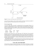
Figure 16.1 Bull spread expiry payoff profile
likely to increase over the next few months, although within a tightly defined range. The trader
contacts an option dealer and constructs a bull spread with the following components. The net
premium payable on the trade is 3.57. (The currency units are not important here, they could
be pence, cents or any other unit.)
Contract Expiry Strike Premium

Long call on XYZ share 3 months 100 −6.18
Short call on XYZ share 3 months 110 +2.61
Figure 16.1 shows the payoff profile of the bull spread at the expiry of the options. The
maximum loss is the net premium. The potential profit is capped at 6.43 when the share price
is trading at 110, the strike of the short call. The break-even point is reached when the stock is
trading at 103.57. The advantage of this strategy compared to buying the 100 strike call on its
own is that the net premium payable is reduced.
Figure 16.2 takes a rather different perspective on the deal. It looks at the value of the strategy
on the day it is put in place, not at expiry, and assumes that the spot price changes on that day
in the range 70–130, with all the other inputs to pricing the option being constant. If the share
price increases then the trade can be unwound by selling the 100 strike call and buying back
the 110 strike call. The maximum profit is still 6.43 (ignoring the time value of money effects).
The bull spread can also be constructed using put options. In this case it would involve
selling an in-the-money put struck at 110 and buying an out-of-the-money put struck at 100.
The advantage here is that net premium would be received rather than paid at the outset,
although taking the time value of money fully into account there is actually no difference in
the ultimate payoff.
BULL POSITION WITH DIGITAL OPTIONS
An alternative to the bull spread is to buy a digital or binary call option on the underlying
share XYZ. The net premium payable on the bull spread in the previous section was 3.57. At
roughly the same cost a dealer could offer a three-month cash-or-nothing (CON) digital call
Option Trading Strategies 163
-8
-3
3
8
70 90 110 130
Spot share price
Profit/loss
Figure 16.2 Bull spread profit and loss on the initial trade date

-10
-5
0
5
10
90 100 110 120
Share price at expiry
Profit/loss
Figure 16.3 Profit/loss at expiry on digital call option with strike 105 and cash payout 10
option on the share struck at 105 and with a cash payout of 10. The CON call works as follows:
if at expiry the share price is above 105 and the option is in-the-money then the payout is 10;
otherwise it is zero. Figure 16.3 illustrates the position at expiry. The net profit and loss is the
payout (either 0 or 10) less the premium. The maximum profit is 10 less the premium while
the maximum loss is simply the premium.
In this case the premium on the digital option is roughly the same as for the bull spread, the
maximum loss and the maximum profit at expiry are about the same, but the nature of the bet
is a little different. The digital option is for someone who is convinced that the share price is
going to be trading above (but not much above) 105 at expiry. If it is in the range 100 to 105
the CON call pays out nothing at all – unlike the bull spread – but if the spot is higher than
164 Derivatives Demystified
0
5
10
15
20
90 95 100 105 110 115 120
Spot price of share
Value
105 CON call
105 vanilla call

Figure 16.4 Value of a cash-or-nothing call for different spot prices
105 the entire cash payout of 10 is due. The payout on the CON call could be increased, but
at the expense of additional premium. For example, a cash-or-nothing call with similar terms
but a payout of 20 would cost about twice as much in premium.
The behaviour of a digital option in response to changes in the spot price of the underlying
is interesting. This is illustrated in Figure 16.4. The dotted line in the graph shows the value of
a 105 strike standard or vanilla call option. The solid line is a 105 strike cash-or-nothing call
with a payout of 10. In both cases there are three months to expiry. As the share price increases,
the value of the vanilla call continues to rise and begins to behave rather like a long position
in the underlying. However, the value of the CON call converges on the cash payout (actually
its present value). The probability of exercise is approaching 100% but the payout is fixed at
10 and cannot be any higher regardless of the value of the underlying in the spot market.
There are many other variants available. For example, an asset-or-nothing (AON) option
pays out the value of the underlying asset if it expires in-the-money, otherwise nothing. In
other cases binary options are structured such that they only pay out if the underlying has hit
a threshold or barrier level during a defined period of time.
BEAR SPREAD
A bear spread gains from a fall in the value of the underlying but with limited profit and loss
potential. In the following example the strategy is assembled using European puts on the same
underlying share considered in the previous sections with a spot price of 100. The net premium
payable on the trade is 2.22, which is also the maximum loss. The maximum profit is achieved
when the underlying share is trading at 95. Below that level any gains on the long 100 strike put
are offset by losses on the short 95 strike put. The expiry payoff profile is shown in Figure 16.5.
Contract Expiry Strike Premium
Long put 3 months 100 −5.68
Short put 3 months 95 +3.46
Option Trading Strategies 165
Table 16.1 Greeks for the bear spread
Theta Vega Rho
Option Delta Gamma (1day) (1%) (1%)

Long 100 put −0.455 0.026 −0.029 0.197 −0.128
Short 95 put 0.325 −0.024 0.027 −0.179 0.090
Net: bear spread −0.130 0.002 −0.002 0.018 −0.038
-5
0
5
90 95 100 105
Share price at expiry
Profit/loss
Figure 16.5 Bear spread expiry payoff profile
It is not necessary, of course, to maintain a position like this all the way to the expiry of the
two options. It could be closed out at any point by selling a 100 strike put and buying a 95
strike put on the same underlying with the same time to expiry. Whether this realizes a profit
or a loss depends on what has happened to the share price in the meantime, and to changes in
the other factors that determine the values of the two options.
To give an idea of the exposures that are involved, Table 16.1 shows the values of the ‘Greeks’
for the long 100 put, the short 95 call, and the net of these values. (For more information on
the Greeks and how they are used by traders see Chapters 14 and 15.)
The Greeks for the bear spread are the sums of the values of the components of the strategy.
As always, the assumption is that all other inputs to the pricing model remain constant. For
example, the delta assumes that the time to expiry, volatility and net carry remain the same,
and only the spot price of the underlying is changed. The vega assumes that the spot, the time
to expiry and the carry are held constant and only the volatility is changed. The values in
Table 16.1 are interpreted as follows (again, the units might be pence, cents or some other
small unit):
r
Delta −0.13. For a small rise (fall) in the price of the underlying of 1 unit the bear spread
shows a loss (a profit) of approximately 0.13 units per share. The fact that delta is negative
indicates that this is a bear strategy – it profits from a fall in the share price.
r

Gamma 0.002. For a small rise of 1 unit in the price of the underlying the delta will change
from −0.13 to −0.13 + 0.002 =−0.128. For a fall of 1 unit in the underlying the delta will
move to −0.13 − 0.002 =−0.132.
166 Derivatives Demystified
r
Theta −0.002. If one day elapses (all other factors remaining constant) the bear spread will
lose approximately 0.002 units in value. The strategy will suffer a little from time value
decay though not to any great extent. It consists of a long and a short three-month option
and the theta effects more-or-less cancel out.
r
Vega 0.018. If volatility increases (decreases) by 1% p.a. the bear spread will increase
(decrease) in value by 0.018 units. The strategy is not particularly sensitive to changes in
volatility.
r
Rho −0.038. If interest rates rise (fall) by 1% p.a. the bear spread will decrease (increase)
in value by 0.038 units. Again the rho is not high. The values on the short and long puts just
about cancel out.
The key exposure with this trade is the negative delta. It tells us that this is indeed a bear
strategy. The other Greeks are not high values, although the slightly positive gamma may be a
small benefit. When the gamma on an option strategy is positive this is an example of what is
sometimes called a ‘right-way’ exposure. This means that if the price of the underlying falls
the strategy either becomes more of a short position or less of a long position, and if the price
rises it becomes more of a long position or less of a short position. However, the gamma effect
is rather limited in this example since one option was bought and another was sold.
A more clear-cut example of a positive gamma trade would consist of buying a call that is
at-the-money and approaching expiry (a put would display similar characteristics). The delta
of the call will be around plus 0.5 and the gamma positive. It will behave rather like a position
in half a share. But if the spot price falls the delta will be less positive, to the limit of zero, at
which point there is no effective exposure to the share price, and if the spot rises the delta will
become more positive, to the limit of 1 or 100%, at which point the call will behave like a long

position in the share. Later examples in this chapter show that negative gamma positions are
‘wrong way’ exposures. Whether the underlying rises or falls, the exposure to changes in the
price of the underlying tends to move in exactly the wrong direction.
PUT OR BEAR RATIO SPREAD
In the spread trades examined so far in thischapter, a long call or put on oneshareis balanced out
by a short call or put also on one share. It is possible to construct spread trades using different
ratios. The ratio spread trade shown below uses European put options. The underlying is the
same as before and the spot price is 100. The net premium payable is 0.8 (again, the units
could be pence, cents or in some other currency).
Contract Expiry Strike Premium per share Total premium
Long put on 1 XYZ share 3 months 100 −5.68 −5.68
Short put on 2 XYZ shares 3 months 92 +2.44 +4.88
Figure 16.6 shows the expiry payoff profile. At a spot price of 100 and above, all the options
expire worthless. The overall loss is the net premium. Below 100 the long 95 strike put is
in-the-money. The maximum profit of 7.2 is reached when the share price is at 92. It consists
of 8 intrinsic value on the long 100 strike put, less the net premium. Below 92 the short put
comes into effect. However, since it is written on two shares in this case, the line does not
flatten out but falls at a 45 degree angle.
The bear ratio spread is a useful strategy when a trader believes the share price is likely to
fall, but to a limited extent. The loss is restricted if the share price actually rises. However the
Option Trading Strategies 167
-15
-10
-5
0
5
10
15
75 80 85 90 95 100 105
Share price at expiry

Profit/loss
Maximum profit = 7.2
Figure 16.6 Bear ratio spread expiry payoff profile
potential losses if it crashes are quite considerable. At a share price of zero the loss on the
strategy is 84.8. The rate of loss depends on the ratio of options bought and sold. For example,
the trader could increase the proportion to 1:3. This is a much more risky trade, although in
this example net premium would be received at the outset.
LONG STRADDLE
A long straddle is essentially a bet on rising volatility levels. It consists of a long call and a
long put on the same underlying with the same strike and the same time to expiry. The strike
is often set around the at-the-money level, as in the following example, which uses the same
underlying share from previous sections, trading at 100 in the spot market.
Contract Expiry Strike Premium
Long call 3 months 100 −6.18
Long put 3 months 100 −5.68
The disadvantage of the trade is that two lots of premium have to be paid, totalling 11.86. On
the other hand, this is the maximum loss. Figure 16.7 shows the expiry payoff profile. The
break-even points are reached when the underlying is trading at 88.14 or at 111.86. As long as
the price has broken out of that range, in either direction, the strategy shows a profit. The trade
is suitable for someone who considers that the share is set to rise or fall sharply over the next
few months, but is not sure of the direction the movement will take. The stimulus could be
the immanent release of financial results that are likely to impact on the share price, positively
or negatively; or simply a period of uncertainty ahead, which will move the price out of its
current trading range.
A long straddle is long volatility trade – the vega is positive. In other words (all other factors
remaining constant), if the volatility assumption used to price the two options rises, they will
increase in value and the long straddle will move into profit.
The delta at the outset, with at-the-money options, is normally quite close to zero. The
gamma is positive which means that it is a ‘right-way’ exposure. If the spot price continues to
168 Derivatives Demystified

-25
-15
-5
5
15
25
75 85 95 105 115 125
Share price at expiry
Profit/loss
Figure 16.7 Long straddle expiry payoff profile
-25
-15
-5
5
15
25
75 85 95 105 115 125
Spot share price
Profit/loss
At outset
1 month later, volatility
down 5%
Figure 16.8 Profit/loss on straddle in response to changes in the spot price
rise, the straddle will become delta positive, i.e. it will behave increasingly like a long position
in the underlying. If the spot continues to fall, it will become delta negative, i.e. it will behave
increasingly like a short position. Unfortunately the strategy is normally also theta negative so
that it tends to suffer from time value decay.
The solid line in Figure 16.8 shows how the profit and loss on the strategy is affected by
changes in the spot price of the underlying on the day it is put in place. Other factors are held
constant – there is still three months to expiry, the volatility and the carry have not changed.

The effects of bid–offer spreads are also ignored. At a spot price of 100 the profit is zero. The
long straddle could be sold back into the market for exactly the same premium at which it was
purchased. But if the spot price rises, the call will move increasingly in-the-money. The put
Option Trading Strategies 169
will lose value, but the maximum loss is the initial premium paid. Similarly, if the spot falls
the put will move in-the-money but the loss on the call is restricted to the premium paid.
The dotted line in Figure 16.8 shows the profit and loss on the straddle after one month
has elapsed and with the assumption that volatility has declined by 5%. The curve has shifted
downwards because the two options have lost time value. Roughly speaking, the spot price of
the underlying would have to have risen or fallen by about 11 to compensate for the losses
resulting from falling volatility and time decay (the vega and the theta effects).
CHOOSER OPTION
The problem with the long straddle is that premium has to be paid on both the call and the put.
The strategy tends to suffer from time value decay and is sensitive to declining volatility. The
time decay effect will become more exaggerated if the options are still around the at-the-money
level as the expiry date approaches. One way to reduce the net premium is to buy a chooser
option. Here the buyer has the right to decide, after a set period of time, whether it is to be
a call or a put. The example in this section is based on the same underlying used previously,
trading at 100 in the spot market. The details of the contract are as follows:
Contract Expiry Strike Time to choose Premium
Long chooser 3 months 100 1 month −9.40
After one month the owner must decide whether it is to be a call or a put. In either case the
strike will be 100 and the time remaining to expiry at that point will be two months. Figure 16.9
shows the profit or loss profile for this chooser option on the day it is purchased, in response
to immediate changes in the spot price, with all the other factors that determine its value held
constant. The curve is similar to that for the long straddle.
The value of the long chooser at any time is the value of the call or the put option it can
become, whichever is the greater of the two. If the spot rises (falls) from the initial level it will
behave like a long call (put) since it is most likely that that will be selected. The gamma (the
-25

-15
-5
5
15
25
75 85 95 105 115 125
Spot share price
Profit/loss
Figure 16.9 Profit/loss on chooser option for changes in the spot price
170 Derivatives Demystified
curvature in the graph) is positive. This tells us that we have a ‘right-way’ exposure. The more
the spot price rises (falls) the more the chooser will behave like a long (short) position in the
underlying and its delta will move towards +1(−1).
The chooser might sound like an extremely exotic structure, although in fact it can be
assembled from quite standard components and is therefore quite easily priced. Ignoring the
complications of carry, the chooser just considered could be replicated by buying a three-month
put and a one-month call, both struck at 100.
SHORT STRADDLE
A short straddle consists of a short call and put on the same underlying with the same strike
and the same time to expiry. It is a short volatility (short vega) trade, since if volatility declines
then (all other factors remaining constant) both options will fall in value. The short straddle
can then be closed out by repurchasing the options for less than the premium at which they
were sold. To illustrate the nature of the strategy, we will take the exact reverse of the long
straddle deal previously discussed. The underlying is the same and is trading at 100.
Contract Expiry Strike Premium
Short call 3 months 100 +6.18
Short put 3 months 100 +5.68
Figure 16.10 shows the expiry payoff profile. The maximum profit is the combined premium,
achieved when the underlying is trading at 100. The seller of the straddle is looking for a dull
market in which the underlying trades in a narrow range around the original spot price of 100.

As long as the underlying is trading in a range somewhere between 88 and 112 the strategy
will make a profit at expiry.
Next, the solid line in Figure 16.11 shows the profit and loss on the short straddle at the outset,
when it has just been sold, in response to immediate changes in the spot price of the underlying.
When the underlying is trading at 100 the strategy is approximately delta neutral, which means
-25
-15
-5
5
15
25
75 85 95 105 115 125
Share price at expiry
Profit/loss
Figure 16.10 Expiry payoff profile of short straddle
Option Trading Strategies 171
-25
-15
-5
5
15
25
75 85 95 105 115 125
Spot share price
Profit/loss
At outset
After 1 month, volatility
down 5%
Figure 16.11 Profit/loss on short straddle for changes in the spot price
that for small movements in the spot the profits and losses net out to approximately zero. There

is no directional exposure to small changes in the price of the underlying. If the share price rises
a little, the short call will move into loss; it would cost more to repurchase than the premium at
which it was sold. However, the put option will move out-of-the-money and become slightly
cheaper to repurchase. Similarly, if the share price falls a little, then losses on the short put are
offset by gains on the short call.
However, the shape of the curvature in the graph reveals the fact that this is a negative gamma
position. This is a classic ‘wrong-way’ exposure. If the share price rises sharply the delta will
become negative and the losses on the short call will greatly exceed the profit on the short
put (the maximum of which is the initial premium at which it was sold). If the share price
continues to rise the delta of the strategy will become increasingly negative and converge on
−1or−100%. At that point the straddle behaves just like a short position in the underlying.
Similarly, if the share price falls, the delta of the straddle will become increasingly positive.
The losses on the put will exceed the gains on the call. Eventually the straddle will behave just
like a long position in the underlying.
Figure 16.11 shows clearly that the trade loses money if the market moves in either direction,
except if the movement is very small. How, then, does it make money? The answer is provided
by the dotted line in the graph, which shows the profit and loss profile after one month has
elapsed, assuming a 5% drop in volatility. As long as the spot price has not changed by more
than about 11 in either direction, the short straddle is in profit, since it can be repurchased for
less than the premium at which it was sold. A short straddle is usually theta positive and as
time goes by both options become cheaper to repurchase. It is also vega negative; if volatility
declines both options lose value.
MANAGING THE GAMMA RISK
The major risk involved in selling a straddle is the negative gamma. As we have seen, this is a
‘wrong way’ exposure. The higher the gamma, the more quickly the delta neutrality will break
down, and the faster the strategy will lose money as the spot price of the underlying fluctuates.
172 Derivatives Demystified
-15
-5
5

15
85 95 105 115
Share price at expiry
Profit/loss
Maximum profit = 7.36
Figure 16.12 Limiting the potential losses on a short straddle
One way to reduce the risk is to sell a straddle and at the same time buy out-of-the-money
call and put options. Figure 16.12 shows the expiry payoff profile of the short straddle struck
at 100 combined with a long call struck at 110 and a long put struck at 90. The straddle is sold
for a premium of 11.86. The premium paid on the long call and put combined is 4.5. Therefore,
the net premium received this time is only 7.36, which is also the maximum profit that can be
achieved on the strategy.
The effect of buying the out-of-the-money call and put is to limit the potential losses on the
combined strategy. It also has the effect of reducing the negative gamma, which means from a
trading perspective that the trade will stay approximately delta neutral for fairly large swings
in the spot price of the underlying. The problem with this solution is that it costs premium to
buy the two options, which reduces the available profit. (The strategy is sometimes called an
iron butterfly.)
Another way to try to combat the negative gamma on a short straddle is to monitor the position
and manage the risk dynamically. For example, if the spot price of the underlying rises, the
short straddle will become delta negative and the losses on the position will accelerate, as
Figure 16.11 illustrates. This can be combated by ‘buying delta’, e.g. buying some of the
underlying. This helps to neutralize losses arising from further increases in the share price.
There is, however, a potential difficulty. If the spot price subsequently falls back again, the
shares that were purchased to achieve delta neutrality will no longer be required. They would
have to be sold for less than the purchase price, realizing a loss.
The same thing would happen in reverse, if the underlying share price fell. The short straddle
would become delta positive, like a long position in the stock. One way to combat this is to
short the underlying, but if the spot price subsequently increased then the short position would
have to be closed out at a loss. As we saw in Chapter 15, chasing the delta in this way can be

extremely costly. The lesson is that a trader who sells a straddle has to be confident about the
volatility forecast. If the underlying trades in a narrow range then the risks on the trade can be
managed at reasonable cost and overall a profit will be realized. However, if the underlying
turns out to be much more volatile than forecast, then the losses realized by managing the delta
exposure will exceed the premium charged at the outset.
Option Trading Strategies 173
CALENDAR OR TIME SPREAD
A calendar spread is designed primarily to take advantage of the different rates of time decay on
options with different expiry dates. It is not based on a view on which direction the share price
is likely to move. The delta – the exposure to small changes in the price of the underlying – is
normally quite close to zero. In the following example a three-month call is purchased and a
one-month call is sold on the same underlying, both European-style and struck at-the-money.
The spot price of the underlying is currently 100 and the net premium paid is 2.62.
Contract Expiry Strike Premium
Long call 3 months 100 −6.18
Short call 1 month 100 +3.56
The positive and negative deltas from the long and the short call will cancel out. However the
theta, the rate of time decay, will be different on the two options. The one-month call will lose
value more quickly since it is closer to expiry than the three-month contract. This is beneficial,
since to close out the trade the one-month call has to be repurchased and the three-month
call sold. In this example, with the same input values for the underlying used throughout this
chapter, the net theta on the strategy is about 0.024. This means that if one day elapses (all
other factors remaining constant) the strategy will gain in value by roughly 0.024 units.
However, the rate of time decay on an option is non-linear, so the daily profit increases as
time goes by. For example, if five days elapse the profit is not 5 × 0.024 = 0.12. It is in fact
0.13. To illustrate this effect, Figure 16.13 shows the decay in the time value of each option over
the course of one month starting from the date the strategy is first established. This assumes
that all other inputs are held constant, and in particular that the spot price and volatility are
unchanged throughout.
There are of course drawbacks to the calendar spread strategy. It is gamma negative, because

the negative gamma of the short-dated option exceeds the positive gamma of the longer-dated
0
2
4
6
8
10
01015202530
Days elapsed
Value
3-month call
1-month call
5
Figure 16.13 Time decay on calls with different expiry dates
174 Derivatives Demystified
option. In practical terms this means that the delta neutrality may break down if the spot
price changes to any significant extent, and the position would then be exposed to directional
movements in the value of the underlying.
CHAPTER SUMMARY
Options can be used to take trading positions in the underlying with a wide variety of risk/return
characteristics. A bull spread is a trade with a maximum loss if the price of the underlying falls
and a capped profit if it rises. A bear spread gains from a fall in the price of the underlying but
the profits and losses cannot exceed defined levels. Options can also be combined in different
ratios. Digital or binary options add to the trading strategies available. A cash-or-nothing digital
option pays out a fixed amount of money if it expires in-the-money, otherwise it pays nothing.
Some strategies are designed to take advantage of changes in volatility or the passage of time
rather than directional movements in the underlying. A long straddle profits if volatility rises.
It also tends to suffer from time value decay and costs two lots of premium. A long chooser
option has a similar profile; the buyer has the right to decide after a period of time whether
it is a call or a put. A short straddle gains if volatility declines, all other factors remaining

constant. It is often set up such that there is little exposure to small movements in the price of
the underlying. However, if the price move is substantial the strategy will move into loss. A
calendar spread is designed to exploit the different rates of time decay on options on the same
underlying that have different expiry dates.
17
Convertible and Exchangeable Bonds
INTRODUCTION
A convertible bond (also known as a convert or CB) is a bond that can be converted into a
fixed number of (normally) ordinary shares, at the choice of the investor. The shares are those
of the issuer of the bond. Often conversion can take place during the whole life of the bond
with the exception of short periods. The number of shares it can be converted into is called the
conversion ratio. The current value of those shares is known as the parity or conversion value
of the CB.
An investor in a convertible has the right to return the bond to the issuer and receive shares
according to the conversion ratio. The bond has embedded within it a call option on the
underlying shares, which will increase in value if the share price performs well. The option
is embedded in the sense that it cannot be split off and traded separately from the convertible
bond. It can only be exercised through conversion. When a convertible bond is first issued the
investors do not pay a premium to the issuer for the embedded option. Instead, they receive a
lower coupon or interest rate on the CB than they would on a standard or straight bond from
the same issuer, i.e. one without the conversion feature.
The first cousin of the convertible is the exchangeable bond. This is exchangeable for shares
of a company other than the issuer of the bond. Issuers include companies that hold significant
stakes in other firms (known as cross-shareholdings) who wish to dispose of those stakes in an
orderly and effective manner. They borrow at a relatively cheap rate by selling exchangeable
bonds and, assuming exchange takes place, are spared the need to redeem the bonds for cash.
Other deals are based on the privatization of assets. For example, in July 2003 the German
state-owned development bank KfW issued €5 billion of bonds exchangeable into Deutsche
Telekom shares. The deal was led by Deutsche Bank and JP Morgan.
In some respects an exchangeable bond is the easier of the two to analyse. An investor in a

convertible has two types of exposure to the issuing company. Firstly, he or she is exposed to
changes in the company’s share price, since this will affect the value of the bond. Secondly, the
CB will lose value if the credit rating of the issuing company is cut and/or the market becomes
increasingly concerned about the prospects of a ratings downgrade or outright default. In
practice these factors are likely to be quite closely related. A collapse in a company’s share
price may well be accompanied by a reduction in its credit rating, and the convertible bond
will suffer twice over. The advantage of an exchangeable is that changes to the credit rating
of the issuer are unlikely to be quite so closely correlated with movements in the price of the
shares, since they are those of a separate organization.
One other problem with a CB is that normally upon conversion the issuing company creates
the new shares to deliver to the investors. This has the effect of diluting the value of the existing
equity, since the profits of the company are now distributed more widely. The advantage of an
exchangeable bond is that it is exchangeable for existing shares and there is no dilution as such.
However, this does not mean that there will be no effect at all on the price of the underlying
176 Derivatives Demystified
share when an exchangeable bond issue is announced. The market might regard the bond as
a means of disposing of a large block of shares, albeit deferred to a later date, and this could
depress the share price on the market. In practice the effect can be rather muted, which is
one reason why a company might decide to dispose of surplus cross-shareholdings by issuing
exchangeable bonds rather than through an outright sale of the shares on the stock market.
Collectively, securities such as convertible and exchangeable bonds are known as equity-
linked issues, because their values are tied to the value of a single share or (sometimes) to
a basket of shares. The equity-linked market is now very big business indeed. According to
research firm Dealogic, global convertible issuance reached $165 billion in 2001.
INVESTORS IN CONVERTIBLE BONDS
Buyers of CBs tend to fall into two main categories. The first consists of hedge funds and
traders searching for arbitrage and relative value transactions. If a CB is relatively cheap then
arbitrageurs can buy the bond (thereby acquiring an inexpensive embedded call option) and
hedge out the directional exposure to the underlying by shorting the stock, using the delta
hedging technique explained in Chapter 15. Essentially what remains is a ‘long volatility’

position, i.e. one that profits from significant swings in the price of the underlying share in
either direction, somewhat like the long straddle trade explored in Chapter 16. A CB is also
sensitive to changes in market interest rates and to the credit rating of the issuer. However,
these can be hedged using interest rate and credit default swaps. It is not uncommon for more
than 50% of a CB issue to be taken up by arbitrageurs.
The second category of buyers of CBs are the more traditional or ‘outright’ investors.
These include fund managers who are seeking to generate additional returns by taking an
equity exposure but who also wish to ensure that the value of the capital invested in the
fund is not placed at undue risk. Convertibles offer clear advantages for the more risk-averse
investors.
r
Capital protection. There is no obligation to convert a CB. If the share performs badly a CB
can always be retained as a bond, earning a regular coupon stream and with the principal
or par value repaid at maturity. On a day-to-day basis, even if the value of the embedded
call option has collapsed, a CB will not trade below its value considered purely as a straight
bond. In the market this is sometimes called the CB’s bond floor.
r
Upside potential. On the other hand, if the share performs well then the investor in a CB
can convert into a predetermined quantity of shares at a favourable price. In the jargon of
the market, a CB offers upside potential (because of the embedded call option) but also
downside protection (because of the bond floor).
r
Income enhancement (versus equity). The coupon or interest rate on the CB may be higher
than the dividends an investor could receive if he or she bought the underlying shares, at
least for a period of time. If so, the investor will earn an enhanced income until conversion.
However, if the embedded call is particularly attractive this may not be the case. Some CBs
pay no interest at all.
r
Higher ranking than equity. CBs are higher ranking than straight equity (ordinary shares or
common stock). A company must make interest and principal payments to bond investors

before the ordinary shareholders are paid anything.
r
Equity-like bond. Professional investors managing fixed-income funds can face restrictions
on purchasing ordinary shares. The advantage of a CB is that it is structured as a bond
Convertible and Exchangeable Bonds 177
although it has an equity-linked return. If the share price rises the convertible will also
increase in value.
Research notes issued by CB analysts in investment banks and aimed at the more traditional
investor group normally discuss the ‘equity story’. In other words, they explain why the analyst
believes that the share price has the potential to increase over some defined investment horizon.
Since the value of the CB is linked to the share price, such an investor will not buy the convertible
unless he or she feels positive about the issuing company and is convinced that its shares have
profit potential.
Typically, the note will also explain the kind of return the investor can expect to achieve
on the CB for given changes in the price of the underlying share. This is often called the
participation rate, and the concept will be explored further in a later section of this chapter.
The research note may also discuss the level of capital protection investors can expect from the
CB and compare this with the potential losses that could be suffered if the underlying shares
are purchased. Techniques for valuing convertible bonds are now more widely understood than
previously and the note will probably also refer to the fair value of the call option embedded
in the CB (established using a pricing model).
ISSUERS OF CONVERTIBLE BONDS
Historically CB issuance in the USA was dominated by high-growth companies with lower
credit ratings, especially in the technology and biotechnology sectors. In recent times more
highly-rated issuers have been attracted to the market as the appetite among investors for
equity-linked bonds has increased. Something of the reverse process has occurred in Europe,
with increased sub-investment grade issuance in recent years.
A lower-rated corporate may find it difficult to obtain an acceptable price for selling its
shares. The stock may be perceived by investors as too risky. On the other hand, if it issued
regular or straight bonds the coupon rate demanded by investors may be too high. Or there may

be no takers at all. If so, the company might find that it can raise capital more effectively by
tapping the convertible bond market. A CB provides investors with a good measure of capital
protection in the shape of the bond floor, while offering the prospects of attractive returns if
the share price performs well. In addition, if the issue is keenly priced, it will attract hedge
funds and other traders seeking to construct arbitrage strategies. In summary, CBs can provide
a useful source of capital for companies. There are a number of potential advantages for the
issuer compared to selling shares or regular straight bonds.
r
Cheaper debt. Because investors have an option to convert into shares, the coupon paid by
the issuer of a CB will be less than the company would have to pay on regular or straight
bonds (without the conversion feature). In addition, issuance costs are usually lower and it
is not normally essential to obtain a credit rating.
r
Selling equity at a premium. The conversion price of a CB is what it would cost an investor
to acquire a share by purchasing and then converting the bond. When a CB is issued the
conversion price can be set at a premium of 25% and more to the price of the share in the
cash market. (Recently there has been a trend towards very high premiums, sometimes over
50%.) Investors accept this because they believe there is a good chance that the share price
will rise by at least this percentage over the life of the bond. For the issuer this is equivalent
to selling shares substantially above the level of the share price at issue (assuming the bonds
are converted).
178 Derivatives Demystified
r
Tax deductibility. Usually companies can offset interest payments against tax, but not div-
idends. A corporate that issues a CB can have the benefit of this so-called tax shield until
such time as the investors decide to convert and the company issues them with shares.
r
Weaker credits. The CB market can help lower credit-rated corporates tap the capital markets.
In such cases the share price is often highly volatile which increases the potential payout
from the embedded call and can make the CB attractive to hedge funds.

CB MEASURES OF VALUE
In order to explore the nature of convertible bonds further we will take a simple example and
consider some valuation issues, in particular the relationship between the value of a CB and
the price of the underlying share. The CB we will consider was issued some time ago at par, i.e.
$100, and now has five years remaining until maturity. Further details are given in Table 17.1.
When the CB was first issued, the coupon rate was set below that for a straight bond. So
its value at issue considered as a bond (i.e. the present value of the interest and principal cash
flows) was actually less than $100. However, investors were prepared to buy the CB at par
because of the value of the embedded call option. At issue, typically somewhere around 75%
of the value of a CB consists in bond value and the rest is option value.
In this example, we are looking at the value of the CB not at issue, but some time later and
with five years remaining to maturity. We will assume that the required return on the market
for straight debt of this credit rating is now 5% p.a., exactly the same as the coupon rate on the
CB. This means that the bond value of the CB is now exactly par, i.e. $100. The CB should
not trade below its bond value (also known as its bond floor) since this represents the value in
today’s money of the future interest and principal cash flows. Does this mean that the CB now
is only worth $100? The answer depends on the current share price. Suppose that the market
cash price of the share is now $5. This allows us to calculate the bond’s parity or conversion
value.
Parity or conversion value now = $5 × 25 = $125
Parity measures the equity value of the CB. In other words, it measures the current value of the
package of shares into which the bond can be converted. Just as a CB should not trade below its
bond value, it should not be possible to purchase a CB for less than its parity value, assuming
that immediate conversion is permitted. The reason once again is the possibility of arbitrage.
If we could buy the bond for less than $125 and immediately convert into shares worth $125
we would make a risk-free profit. Market forces should prevent this from happening and the
CB should trade for at least its parity value. Parity is related to the modern concept of intrinsic
value. The CB should not trade below its parity value in the same way that an American-style
call option should not trade below its intrinsic value.
Table 17.1 Details of the bond

Issuer: XYZ inc.
Par or nominal value: $100
Conversion ratio: Convertible into 25 XYZ shares
Coupon rate: 5% p.a.
Conversion dates: Any business day up to maturity
Convertible and Exchangeable Bonds 179
Does this mean that the XYZ convertible should only trade at its parity value? No, for at
least two reasons. Firstly, unlike an investment in the underlying shares, the CB offers capital
protection in the shape of the bond floor. Secondly, the CB still has five years to maturity
and there is a good chance that the share price will increase over that time, which would
drive the value of the CB up still further. The CB contains an embedded call option on 25
underlying XYZ shares with five years to expiry, which has significant time value. The amount
that investors are prepared to pay over the parity or conversion value of a convertible bond is
called conversion premium or premium-over-parity. Suppose the XYZ share price is $5 and the
parity value of the convertible bond is $125. If the CB is trading for (say) $156 in the market
then its conversion premium is calculated as follows:
Conversion premium = $156 − $125 = $31
Percentage conversion premium = $31/$125 = 24.8%
Conversion premium per share = $31/25 shares = $1.24
If an investor buys the CB for $156 and immediately converts, then the cost of buying the
equity through this means is $6.24 per share. This is $1.24 or 24.8% more than it would cost
to buy the share in the cash market. It also means that the share price would have to rise by at
least 24.8% before it would make any sense for the investor to convert the bond into shares.
Note that the term ‘conversion premium’ does not quite mean the same thing as the modern
expression ‘option premium’ though it is related, as we will see in more detail in the next
section.
CONVERSION PREMIUM AND PARITY
To help to explore these issues further, Figure 17.1 illustrates the basic relationship between
bond value, parity and conversion premium for the XYZ bond. The bond value (bond floor) is
0

50
100
150
200
250
300
12345678910
XYZ share price $
Value $
Bond floor
Parity
CB value
Figure 17.1 CB value, parity and bond floor
180 Derivatives Demystified
assumed to be $100 and there are now five years to maturity. The CB has been priced assuming
a 30% p.a. volatility for the underlying shares and assuming that they pay no dividends. Since
the CB has a 5% coupon this means that an investor has an income advantage in holding
the convertible bond. In the graph parity is shown as a solid diagonal line. Since the bond is
always convertible into exactly 25 shares the relationship between the share price and parity
is perfectly linear. If the share price is very low at (say) $1, then the parity or equity value
of the bond is only $25. At a share price of $10 parity is $250. The bond floor is shown as a
horizontal line; the bond value of the CB is taken to be $100 whatever the current share price
level. The total CB value is a curved dotted line.
The difference between the total CB value and the parity value of the bond at a given share
price is the conversion premium. There are two main factors that determine the conversion
premium for this bond, and the one that predominates depends on where the share price is
trading.
1. Bond floor. At very low share prices the value of the CB reverts to its bond floor. It is
extremely unlikely that it will ever be converted and the value of the embedded call option
is almost zero. It is deeply out-of-the-money. At this level conversion premium is largely

determined by the fact that the holder of the CB is not obliged to convert and has the comfort
of being able to retain the security as a pure bond investment. If the investor owned shares
instead, then the value of those shares would be sliding down the diagonal parity line.
2. Embedded call. At very high share prices the value of the CB converges on its parity value.
The CB starts to trade like a package of 25 shares since it is almost 100% certain that it will
be converted. There is very little uncertainty about the eventual outcome. The embedded
call is deeply in-the-money and (as is the case with such options) the time value component
is very low.
OTHER FACTORS AFFECTING CB VALUE
It is often said in the markets that ‘a CB is just a bond with an option’. This is a good enough
definition when explaining the basic structure of the instrument, but it can be a little misleading
in practice and needs a few words of qualification. Firstly, a CB can normally be converted
over a period of time and not just at maturity. The pricing methodology has to take into account
the fact that it should not trade at less than its parity value, otherwise arbitrage opportunities
would be created.
Secondly, when a CB is converted the issuing company normally creates new shares. This has
the unfortunate effect of diluting the value of the equity. Thirdly, we assumed in constructing
the graph in Figure 17.1 that the bond floor of the CB (its value considered purely as a straight
bond) is unaffected by changes in the share price. In practice this is unlikely. A CB is issued
by a company and the bond is convertible into the shares of the same company. If the share
price collapses we might well expect the bond floor to shift downwards because of fears that
the company might default on its debt or declare bankruptcy. In assessing the value of the CB
we should properly make some assumptions about the relationship between movements in the
share price and the value of the bond floor.
We noted before that an exchangeable bond is in some ways easier to analyse. The bond is
issued by one company but is exchangeable for the shares of another. This means that the credit
risk on the bond and the value of the shares are not quite so intimately related. An investor
who is weighing up the ‘equity story’ on the shares and considering whether they offer profit
Convertible and Exchangeable Bonds 181
potential can assess this possibility quite separately from any questions about the credit or

default risk on the bond. Exchangeables are often issued by highly-rated organizations that
wish to sell off and ‘monetize’ the value of stakes in other businesses that were acquired for
historical reasons that are no longer relevant.
As a final valuation issue, it is important to understand that many CB issues incorporate
complex early redemption provisions. The issuer may have the power to ‘call’ the bond back
early at par or just above if it is trading above a certain trigger level for a period of time.
To return to our example, suppose that XYZ company has the right to retire the CB at par
if it trades above $175 for a period of two weeks. This would occur if the XYZ share price
had risen sharply and driven up the parity value of the CB. By putting out the ‘call’ or early
retirement notice the company is effectively forcing investors to convert. It could then issue
new convertible bonds at a conversion price set above the current share price. The call feature
is obviously an advantage to the issuer and a disadvantage to the investor and this fact should
be reflected in the market value of the CB.
The position on early retirement of CBs tends to be quite complex and to require some fairly
sophisticated valuation. A convertible may incorporate a number of separate call features, some
of which allow the issuer to ‘call’ the bond back early after a period of time whatever its value
in the market; and others which are only triggered when the CB trades above a certain level for
a period of time. In addition, the terms of the bond may grant the investor the right in certain
circumstances to ‘put’ or return the bond back to the investor for cash. This is obviously an
advantage to the investor, who can have his or her capital returned early if the CB is found to be a
poor investment. As such, the put feature should be reflected in the market value of the security.
PARTICIPATION RATES
The participation rate of a CB tells an investor the rate of return he or she might expect to
achieve for a given change in the share price, other factors remaining constant. To explore this
concept further, we return to the XYZ convertible bond analysed in the previous sections. The
details of the bond were as given in Table 17.2 (there are no call or put features).
If we imagine that the XYZ share price is currently $5, then the parity value of the CB
is $125. However, the bond still has five years to maturity; it offers a 5% coupon while the
underlying share pays no dividends; and unlike an investment in the share the bond offers
capital protection. For all these reasons the CB will be worth more than its parity value.

Suppose that the CB is in fact trading at $156 in the market. Table 17.3 shows what would (in
theory) happen to the value of the CB if the share price suddenly jumped to $6 or fell to $4.The
method employed here was to revalue the embedded call assuming that the only variable that
changes is the underlying share price. The table also shows the percentage change in the share
price starting from $5 and the resulting percentage change in the value of the CB.
Table 17.2 Details of the bond
Issuer: XYZ inc.
Par or nominal value: $100
Conversion ratio: Convertible into 25 XYZ shares
Coupon rate: 5% p.a.
Remaining maturity: 5 years
Conversion dates: Any business day up to maturity
182 Derivatives Demystified
Table 17.3 Participation rate calculations for convertible bond
Share price ($) Change (%) CB value ($) Change (%) Participation (%)
4 −20 136 −13 64
5 0 156 0 0
6 20 178 14.1 71
100
150
200
4
Share price $
Value $
Shares value
CB value
5
6
Figure 17.2 CB compared with investment in the underlying shares
The table also shows that if the share price rises from $5 to $6 (an increase of 20%) the

percentage rise in the value of the CB is about 14%. An investor who bought the CB at $156
would only achieve 71% of the gains that he or she would have achieved if the money had
been used instead to buy XYZ shares. This is the upside participation rate, the rate at which
the CB investor would participate in the rise in the share to a target level of $6.
Upside participation rate = 14.1%/20% = 71%
On the other hand, if the share price falls to $4 then an investor in the CB would only suffer
64% of the losses he or she would have made on the underlying shares; and if the share price
collapses, the value of the CB will revert to its bond floor. The dotted line in Figure 17.2
illustrates how, in theory, the CB will change in value for a given change in the underlying
share price. The solid line shows what would happen if, rather than investing in the CB, an
investor used the money to buy XYZ shares in the cash market at $5 each.
MANDATORILY CONVERTIBLES AND EXCHANGEABLES
A mandatorily convertible (MC) is, as the name suggests, a bond which the investor must
convert on a future date. As an example, Deutsche Telekom launched a €2.3 billion MC bond
in February 2003 in order to reduce its debt burden, which then amounted to over €60 billion.
The deal was successful and about three times over-subscribed.
Convertible and Exchangeable Bonds 183
Table 17.4 The terms of the ME bond
Bond issue price: $100
Maturity: 1 year
Exchange ratio: Each bond is mandatorily exchangeable
into one share at maturity.
Coupon rate: 0%
A mandatorily exchangeable (ME) might be issued by a company that has a cross-holding
of shares in another business which it definitely wishes to dispose of on some future date. In
effect the bond is a deferred or forward sale of the shares but with the cash proceeds received
up front. There are many reasons why the company might wish to dispose of the shares in this
way rather than by simply selling them in a cash market transaction.
r
It may be more tax efficient.

r
The market impact may be lower – announcing a cash market sale of a large block of shares
could seriously affect the market price. This would be particularly painful if the company
intended to retain some of its holding.
r
There may be legal or regulatory restrictions on selling the shares until some period of time
has elapsed.
A very simple example may help to explain the basic idea. A more detailed (and realistic)
example is given in the next section. Let us suppose that a company owns a block of shares it
wishes to dispose of in one year’s time. The current share price is $100, the annual dividend
is $1 per share and the one-year interest rate is 5% p.a. The one-year fair forward price,
established using the cash-and-carry method explained in Chapter 2, is therefore $100 + $5
− $1 = $104.
The company could go to a dealer and agree to sell the shares forward in an over-the-counter
transaction. If it contracts the forward deal at $104 per share then it could borrow money today
against the future cash flow guaranteed by this transaction. It is due to receive $104 per share
in one year’s time so, at an interest rate of 5% p.a., it could borrow just over $99 per share
today. Alternatively, rather than agree the forward, the company might get a better deal by
selling a mandatorily exchangeable bond to investors through the public markets. The terms
of the bond might be as shown in Table 17.4.
In this structure, investors buy a bond for $100 and one year later they receive (without any
choice) one share per bond. In effect, the company is selling the shares to the bond investors
in a year’s time but receiving the proceeds up front. The advantage is that it is receiving $100
per share up front rather than the $99 that could be borrowed against a forward sale of the
shares. In practice mandatorily convertible and exchangeable bonds can be constructed such
that investors have some protection against a fall in the share price. Alternatively, there is no
capital protection as such, but investors receive an attractive coupon in compensation for the
requirement to exchange the bond for shares. An example is explored in the next section.
STRUCTURING A MANDATORILY EXCHANGEABLE
The advantage of these types of deals is that they can be packaged in different ways to make

them more attractive to investors. One technique used by investment banks is to issue a ME bond
with a coupon rate that is appreciably higher than the dividends investors would receive if they
bought the underlying shares in the cash market. However, investors are obliged to exchange