essentials of investments with s p bind in card phần 8 pps
Bạn đang xem bản rút gọn của tài liệu. Xem và tải ngay bản đầy đủ của tài liệu tại đây (1.73 MB, 77 trang )
Bodie−Kane−Marcus:
Essentials of Investments,
Fifth Edition
V. Derivative Markets 15. Option Valuation
© The McGraw−Hill
Companies, 2003
considered relatively expensive because a higher standard deviation is required to justify its
price. The analyst might consider buying the option with the lower implied volatility and writ-
ing the option with the higher implied volatility.
The Black-Scholes call-option valuation formula, as well as implied volatilities, are eas-
ily calculated using an Excel spreadsheet, as in Figure 15.4. The model inputs are listed in
15 Option Valuation 545
TABLE 15.2
(concluded)
dN(d ) dN(d ) dN(d )
0.06 0.5239 0.86 0.8051 1.66 0.9515
0.08 0.5319 0.88 0.8106 1.68 0.9535
0.10 0.5398 0.90 0.8159 1.70 0.9554
0.12 0.5478 0.92 0.8212 1.72 0.9573
0.14 0.5557 0.94 0.8264 1.74 0.9591
0.16 0.5636 0.96 0.8315 1.76 0.9608
0.18 0.5714 0.98 0.8365 1.78 0.9625
0.20 0.5793 1.00 0.8414 1.80 0.9641
0.22 0.5871 1.02 0.8461 1.82 0.9656
0.24 0.5948 1.04 0.8508 1.84 0.9671
0.26 0.6026 1.06 0.8554 1.86 0.9686
0.28 0.6103 1.08 0.8599 1.88 0.9699
0.30 0.6179 1.10 0.8643 1.90 0.9713
0.32 0.6255 1.12 0.8686 1.92 0.9726
0.34 0.6331 1.14 0.8729 1.94 0.9738
0.36 0.6406 1.16 0.8770 1.96 0.9750
0.38 0.6480 1.18 0.8810 1.98 0.9761
0.40 0.6554 1.20 0.8849 2.00 0.9772
0.42 0.6628 1.22 0.8888 2.05 0.9798
0.44 0.6700 1.24 0.8925 2.10 0.9821
0.46 0.6773 1.26 0.8962 2.15 0.9842
0.48 0.6844 1.28 0.8997 2.20 0.9861
0.50 0.6915 1.30 0.9032 2.25 0.9878
0.52 0.6985 1.32 0.9066 2.30 0.9893
0.54 0.7054 1.34 0.9099 2.35 0.9906
0.56 0.7123 1.36 0.9131 2.40 0.9918
0.58 0.7191 1.38 0.9162 2.45 0.9929
0.60 0.7258 1.40 0.9192 2.50 0.9938
0.62 0.7324 1.42 0.9222 2.55 0.9946
0.64 0.7389 1.44 0.9251 2.60 0.9953
0.66 0.7454 1.46 0.9279 2.65 0.9960
0.68 0.7518 1.48 0.9306 2.70 0.9965
0.70 0.7580 1.50 0.9332 2.75 0.9970
0.72 0.7642 1.52 0.9357 2.80 0.9974
0.74 0.7704 1.54 0.9382 2.85 0.9978
0.76 0.7764 1.56 0.9406 2.90 0.9981
0.78 0.7823 1.58 0.9429 2.95 0.9984
0.80 0.7882 1.60 0.9452 3.00 0.9986
0.82 0.7939 1.62 0.9474 3.05 0.9989
0.84 0.7996 1.64 0.9495
Bodie−Kane−Marcus:
Essentials of Investments,
Fifth Edition
V. Derivative Markets 15. Option Valuation
© The McGraw−Hill
Companies, 2003
546
column B, and the outputs are given in column E. The formulas for d
1
and d
2
are provided in
the spreadsheet, and the Excel formula NORMSDIST(d
1
) is used to calculate N(d
1
). Cell E6
contains the Black-Scholes call option formula. To compute an implied volatility, we can use
the Solver command from the Tools menu in Excel. Solver asks us to change the value of one
cell to make the value of another cell (called the target cell) equal to a specific value. For ex-
ample, if we observe a call option selling for $7 with other inputs as given in the spreadsheet,
we can use Solver to find the value for cell B2 (the standard deviation of the stock) that will
make the option value in cell E6 equal to $7. In this case, the target cell, E6, is the call price,
and the spreadsheet manipulates cell B2. When you ask the spreadsheet to “Solve,” it finds
that a standard deviation equal to .2783 is consistent with a call price of $7; therefore, 27.83%
would be the call’s implied volatility if it were selling at $7.
7. Consider the call option in Example 15.2 If it sells for $15 rather than the value of
$13.70 found in the example, is its implied volatility more or less than 0.5?
The Put-Call Parity Relationship
So far, we have focused on the pricing of call options. In many important cases, put prices can
be derived simply from the prices of calls. This is because prices of European put and call
EXCEL Applications www.mhhe.com/bkm
Black-Scholes Option Pricing
Figure 15.4 captures a portion of the Excel model “B-S Option.” The model is built to value puts
and calls and extends the discussion to include analysis of intrinsic value and time value of op-
tions. The spreadsheet contains sensitivity analyses on several key variables in the Black-Scholes
pricing model.
You can learn more about this spreadsheet model by using the interactive version available on
our website at www
.mhhe.com/bkm.
>
Concept
CHECK
>
FIGURE 15.4
Spreadsheet to calculate Black-Scholes call-option values
Bodie−Kane−Marcus:
Essentials of Investments,
Fifth Edition
V. Derivative Markets 15. Option Valuation
© The McGraw−Hill
Companies, 2003
options are linked together in an equation known as the put-call parity relationship. Therefore,
once you know the value of a call, put pricing is easy.
To derive the parity relationship, suppose you buy a call option and write a put option, each
with the same exercise price, X, and the same expiration date, T. At expiration, the payoff on
your investment will equal the payoff to the call, minus the payoff that must be made on the
put. The payoff for each option will depend on whether the ultimate stock price, S
T
, exceeds
the exercise price at contract expiration.
S
T
Յ XS
T
Ͼ X
Payoff of call held 0 S
T
Ϫ X
ϪPayoff of put written Ϫ(X Ϫ S
T
)0
Total S
T
Ϫ XS
T
Ϫ X
Figure 15.5 illustrates this payoff pattern. Compare the payoff to that of a portfolio made
up of the stock plus a borrowing position, where the money to be paid back will grow, with
interest, to X dollars at the maturity of the loan. Such a position is a levered equity position in
15 Option Valuation 547
FIGURE 15.5
The payoff pattern of
a long call–short
put position
S
T
Payoff
Payoff
Payoff
X
S
T
S
T
X
Long call
+ Short put
= Leveraged equity
Bodie−Kane−Marcus:
Essentials of Investments,
Fifth Edition
V. Derivative Markets 15. Option Valuation
© The McGraw−Hill
Companies, 2003
which X/(1 ϩ r
f
)
T
dollars is borrowed today (so that X will be repaid at maturity), and S
0
dol-
lars is invested in the stock. The total payoff of the levered equity position is S
T
Ϫ X, the same
as that of the option strategy. Thus, the long call–short put position replicates the levered
equity position. Again, we see that option trading provides leverage.
Because the option portfolio has a payoff identical to that of the levered equity position, the
costs of establishing them must be equal. The net cash outlay necessary to establish the option
position is C Ϫ P: The call is purchased for C, while the written put generates income of P.
Likewise, the levered equity position requires a net cash outlay of S
0
Ϫ X/(1 ϩ r
f
)
T
, the cost of
the stock less the proceeds from borrowing. Equating these costs, we conclude
C Ϫ P ϭ S
0
Ϫ X/(1 ϩ r
f
)
T
(15.2)
Equation 15.2 is called the put-call parity relationship because it represents the proper re-
lationship between put and call prices. If the parity relationship is ever violated, an arbitrage
opportunity arises.
Equation 15.2 actually applies only to options on stocks that pay no dividends before the
maturity date of the option. It also applies only to European options, as the cash flow streams
from the two portfolios represented by the two sides of Equation 15.2 will match only if each
position is held until maturity. If a call and a put may be optimally exercised at different times
548 Part FIVE Derivative Markets
put-call parity
relationship
An equation
representing the
proper relationship
between put and call
prices.
15.3 EXAMPLE
Put-Call
Parity
Suppose you observe the following data for a certain stock.
Stock price $110
Call price (six-month maturity, X ϭ $105) 17
Put price (six-month maturity, X ϭ $105) 5
Risk-free interest rate 10.25% effective annual
yield (5% per 6 months)
We use these data in the put-call parity relationship to see if parity is violated.
C Ϫ P S
0
Ϫ X/(1 ϩ r
f
)
T
17 Ϫ 5 110 Ϫ 105/1.05
12 10
This result, a violation of parity (12 does not equal 10) indicates mispricing and leads to an
arbitrage opportunity. You can buy the relatively cheap portfolio (the stock plus borrowing
position represented on the right-hand side of the equation) and sell the relatively expensive
portfolio (the long call–short put position corresponding to the left-hand side, that is, write a
call and buy a put).
Let’s examine the payoff to this strategy. In six months, the stock will be worth S
T
. The
$100 borrowed will be paid back with interest, resulting in a cash outflow of $105. The writ-
ten call will result in a cash outflow of S
T
Ϫ $105 if S
T
exceeds $105. The purchased put
pays off $105 Ϫ S
T
if the stock price is below $105.
Table 15.3 summarizes the outcome. The immediate cash inflow is $2. In six months, the
various positions provide exactly offsetting cash flows: The $2 inflow is realized risklessly with-
out any offsetting outflows. This is an arbitrage opportunity that investors will pursue on a
large scale until buying and selling pressure restores the parity condition expressed in Equa-
tion 15.2.
Bodie−Kane−Marcus:
Essentials of Investments,
Fifth Edition
V. Derivative Markets 15. Option Valuation
© The McGraw−Hill
Companies, 2003
before their common expiration date, then the equality of payoffs cannot be assured, or even
expected, and the portfolios will have different values.
The extension of the parity condition for European call options on dividend-paying stocks
is, however, straightforward. Problem 22 at the end of the chapter leads you through the
extension of the parity relationship. The more general formulation of the put-call parity con-
dition is
P ϭ C Ϫ S
0
ϩ PV(X) ϩ PV(dividends) (15.3)
where PV(dividends) is the present value of the dividends that will be paid by the stock dur-
ing the life of the option. If the stock does not pay dividends, Equation 15.3 becomes identi-
cal to Equation 15.2.
Notice that this generalization would apply as well to European options on assets other than
stocks. Instead of using dividend income in Equation 15.3, we would let any income paid out
by the underlying asset play the role of the stock dividends. For example, European put and
call options on bonds would satisfy the same parity relationship, except that the bond’s coupon
income would replace the stock’s dividend payments in the parity formula.
Let’s see how well parity works using real data on the Microsoft options in Figure 14.1
from the previous chapter. The April maturity call with exercise price $70 and time to expira-
tion of 105 days cost $4.60 while the corresponding put option cost $5.40. Microsoft was sell-
ing for $68.90, and the annualized 105-day interest rate on this date was 1.6%. Microsoft was
paying no dividends at this time. According to parity, we should find that
P ϭ C ϩ PV(X) Ϫ S
0
ϩ PV(dividends)
5.40 ϭ 4.60 ϩϪ68.90 ϩ 0
5.40 ϭ 4.60 ϩ 69.68 Ϫ 68.90
5.40 ϭ 5.38
So, parity is violated by about $0.02 per share. Is this a big enough difference to exploit? Prob-
ably not. You have to weigh the potential profit against the trading costs of the call, put, and
stock. More important, given the fact that options trade relatively infrequently, this deviation
from parity might not be “real” but may instead be attributable to “stale” (i.e., out-of-date)
price quotes at which you cannot actually trade.
Put Option Valuation
As we saw in Equation 15.3, we can use the put-call parity relationship to value put options
once we know the call option value. Sometimes, however, it is easier to work with a put option
70
(1.016)
105/365
15 Option Valuation 549
TABLE 15.3
Arbitrage strategy
Cash Flow in Six Months
Position Immediate Cash Flow S
T
Ͻ 105 S
T
Ն 105
Buy stock Ϫ110 S
T
S
T
Borrow X/(1 ϩ r
f
)
T
ϭ $100 ϩ100 Ϫ105 Ϫ105
Sell call ϩ17 0 Ϫ(S
T
Ϫ 105)
Buy put Ϫ5 105 Ϫ S
T
0
Total 2 0 0
Bodie−Kane−Marcus:
Essentials of Investments,
Fifth Edition
V. Derivative Markets 15. Option Valuation
© The McGraw−Hill
Companies, 2003
valuation formula directly. The Black-Scholes formula for the value of a European put op-
tion is
3
P ϭ Xe
ϪrT
[1 Ϫ N(d
2
)] Ϫ S
0
e
Ϫ␦T
[1 Ϫ N(d
1
)] (15.4)
Equation 15.4 is valid for European puts. Listed put options are American options that offer
the opportunity of early exercise, however. Because an American option allows its owner to
exercise at any time before the expiration date, it must be worth at least as much as the corre-
sponding European option. However, while Equation 15.4 describes only the lower bound on
the true value of the American put, in many applications the approximation is very accurate.
15.4 USING THE BLACK-SCHOLES FORMULA
Hedge Ratios and the Black-Scholes Formula
In the last chapter, we considered two investments in Microsoft: 100 shares of Microsoft stock
or 700 call options on Microsoft. We saw that the call option position was more sensitive to
swings in Microsoft’s stock price than the all-stock position. To analyze the overall exposure
to a stock price more precisely, however, it is necessary to quantify these relative sensitivities.
A tool that enables us to summarize the overall exposure of portfolios of options with various
exercise prices and times to maturity is the hedge ratio. An option’s hedge ratio is the change
in the price of an option for a $1 increase in the stock price. A call option, therefore, has a pos-
itive hedge ratio, and a put option has a negative hedge ratio. The hedge ratio is commonly
called the option’s delta.
If you were to graph the option value as a function of the stock value as we have done for
a call option in Figure 15.6, the hedge ratio is simply the slope of the value function evaluated
at the current stock price. For example, suppose the slope of the curve at S
0
ϭ $120 equals
0.60. As the stock increases in value by $1, the option increases by approximately $0.60, as
the figure shows.
For every call option written, 0.60 shares of stock would be needed to hedge the investor’s
portfolio. For example, if one writes 10 options and holds six shares of stock, according to the
hedge ratio of 0.6, a $1 increase in stock price will result in a gain of $6 on the stock holdings,
550 Part FIVE Derivative Markets
3
This formula is consistent with the put-call parity relationship, and in fact can be derived from it. If you want to try to
do so, remember to take present values using continuous compounding, and note that when a stock pays a continuous
flow of income in the form of a constant dividend yield, ␦, the present value of that dividend flow is S
0
(1 Ϫ e
Ϫ␦T
).
(Notice that e
Ϫ␦T
approximately equals 1 Ϫ␦T, so the value of the dividend flow is approximately ␦TS
0
.)
15.4 EXAMPLE
Black-Scholes
Put Option
Valuation
Using data from the Black-Scholes call option in Example 15.2 we find that a European put
option on that stock with identical exercise price and time to maturity is worth
$95e
Ϫ.10 ϫ .25
(1 Ϫ .5714) Ϫ $100(1 Ϫ .6664) ϭ $6.35
Notice that this value is consistent with put-call parity:
P ϭ C ϩ PV(X) Ϫ S
0
ϭ 13.70 ϩ 95e
Ϫ.10 ϫ .25
Ϫ 100 ϭ 6.35
As we noted traders can do, we might then compare this formula value to the actual put
price as one step in formulating a trading strategy.
hedge ratio
or delta
The number of shares
of stock required to
hedge the price risk
of holding one option.
Bodie−Kane−Marcus:
Essentials of Investments,
Fifth Edition
V. Derivative Markets 15. Option Valuation
© The McGraw−Hill
Companies, 2003
while the loss on the 10 options written will be 10 ϫ $0.60, an equivalent $6. The stock price
movement leaves total wealth unaltered, which is what a hedged position is intended to do.
The investor holding both the stock and options in proportions dictated by their relative price
movements hedges the portfolio.
Black-Scholes hedge ratios are particularly easy to compute. The hedge ratio for a call is
N(d
1
), while the hedge ratio for a put is N(d
1
) Ϫ 1. We defined N(d
1
) as part of the Black-
Scholes formula in Equation 15.1. Recall that N(d ) stands for the area under the standard nor-
mal curve up to d. Therefore, the call option hedge ratio must be positive and less than 1.0,
while the put option hedge ratio is negative and of smaller absolute value than 1.0.
Figure 15.6 verifies the insight that the slope of the call option valuation function is less
than 1.0, approaching 1.0 only as the stock price becomes extremely large. This tells us that
option values change less than one-for-one with changes in stock prices. Why should this be?
Suppose an option is so far in the money that you are absolutely certain it will be exercised.
In that case, every $1 increase in the stock price would increase the option value by $1. But if
there is a reasonable chance the call option will expire out of the money, even after a moder-
ate stock price gain, a $1 increase in the stock price will not necessarily increase the ultimate
payoff to the call; therefore, the call price will not respond by a full $1.
The fact that hedge ratios are less than 1.0 does not contradict our earlier observation that
options offer leverage and are sensitive to stock price movements. Although dollar move-
ments in option prices are slighter than dollar movements in the stock price, the rate of return
volatility of options remains greater than stock return volatility because options sell at lower
prices. In our example, with the stock selling at $120, and a hedge ratio of 0.6, an option with
exercise price $120 may sell for $5. If the stock price increases to $121, the call price would
be expected to increase by only $0.60, to $5.60. The percentage increase in the option value is
$0.60/$5.00 ϭ 12%, however, while the stock price increase is only $1/$120 ϭ 0.83%. The
ratio of the percent changes is 12%/0.83% ϭ 14.4. For every 1% increase in the stock price,
the option price increases by 14.4%. This ratio, the percent change in option price per percent
change in stock price, is called the option elasticity.
The hedge ratio is an essential tool in portfolio management and control. An example will
show why.
15 Option Valuation 551
FIGURE 15.6
Call option value
and hedge ratio
Value of a call (C )
S
0
40
20
0
120
Slope = .6
option elasticity
The percentage
increase in an
option’s value
given a 1% increase
in the value of the
underlying security.
Bodie−Kane−Marcus:
Essentials of Investments,
Fifth Edition
V. Derivative Markets 15. Option Valuation
© The McGraw−Hill
Companies, 2003
8. What is the elasticity of a put option currently selling for $4 with exercise price
$120, and hedge ratio ؊0.4 if the stock price is currently $122?
Portfolio Insurance
In Chapter 14, we showed that protective put strategies offer a sort of insurance policy on an
asset. The protective put has proven to be extremely popular with investors. Even if the asset
price falls, the put conveys the right to sell the asset for the exercise price, which is a way to
lock in a minimum portfolio value. With an at-the-money put (X ϭ S
0
), the maximum loss that
can be realized is the cost of the put. The asset can be sold for X, which equals its original
price, so even if the asset price falls, the investor’s net loss over the period is just the cost of
the put. If the asset value increases, however, upside potential is unlimited. Figure 15.7 graphs
the profit or loss on a protective put position as a function of the change in the value of the
underlying asset.
While the protective put is a simple and convenient way to achieve portfolio insurance,
that is, to limit the worst-case portfolio rate of return, there are practical difficulties in trying
to insure a portfolio of stocks. First, unless the investor’s portfolio corresponds to a standard
market index for which puts are traded, a put option on the portfolio will not be available for
purchase. And if index puts are used to protect a nonindexed portfolio, tracking error can re-
sult. For example, if the portfolio falls in value while the market index rises, the put will fail
to provide the intended protection. Tracking error limits the investor’s freedom to pursue ac-
tive stock selection because such error will be greater as the managed portfolio departs more
substantially from the market index.
Moreover, the desired horizon of the insurance program must match the maturity of a
traded put option in order to establish the appropriate protective put position. Today, long-term
index options called LEAPS (for Long-Term Equity AnticiPation Securities) trade on the
Chicago Board Options Exchange with maturities of several years. However, in the mid-
1980s, while most investors pursuing insurance programs had horizons of several years, ac-
tively traded puts were limited to maturities of less than a year. Rolling over a sequence of
short-term puts, which might be viewed as a response to this problem, introduces new risks
because the prices at which successive puts will be available in the future are not known today.
Providers of portfolio insurance with horizons of several years, therefore, cannot rely on
the simple expedient of purchasing protective puts for their clients’ portfolios. Instead, they
follow trading strategies that replicate the payoffs to the protective put position.
552 Part FIVE Derivative Markets
15.5 EXAMPLE
Portfolio
Hedge
Ratios
Consider two portfolios, one holding 750 IBM calls and 200 shares of IBM and the other
holding 800 shares of IBM. Which portfolio has greater dollar exposure to IBM price move-
ments? You can answer this question easily using the hedge ratio.
Each option changes in value by H dollars for each dollar change in stock price, where H
stands for the hedge ratio. Thus, if H equals 0.6, the 750 options are equivalent to 450
(ϭ 0.6 ϫ 750) shares in terms of the response of their market value to IBM stock price
movements. The first portfolio has less dollar sensitivity to stock price change because the
450 share-equivalents of the options plus the 200 shares actually held are less than the 800
shares held in the second portfolio.
This is not to say, however, that the first portfolio is less sensitive to the stock’s rate of re-
turn. As we noted in discussing option elasticities, the first portfolio may be of lower total
value than the second, so despite its lower sensitivity in terms of total market value, it might
have greater rate of return sensitivity. Because a call option has a lower market value than
the stock, its price changes more than proportionally with stock price changes, even though
its hedge ratio is less than 1.0.
Concept
CHECK
>
portfolio
insurance
Portfolio
strategies that limit
investment losses
while maintaining
upside potential.
Bodie−Kane−Marcus:
Essentials of Investments,
Fifth Edition
V. Derivative Markets 15. Option Valuation
© The McGraw−Hill
Companies, 2003
Here is the general idea. Even if a put option on the desired portfolio with the desired ex-
piration date does not exist, a theoretical option-pricing model (such as the Black-Scholes
model) can be used to determine how that option’s price would respond to the portfolio’s value
if the option did trade. For example, if stock prices were to fall, the put option would increase
in value. The option model could quantify this relationship. The net exposure of the (hypo-
thetical) protective put portfolio to swings in stock prices is the sum of the exposures of the
two components of the portfolio: the stock and the put. The net exposure of the portfolio
equals the equity exposure less the (offsetting) put option exposure.
We can create “synthetic” protective put positions by holding a quantity of stocks with the
same net exposure to market swings as the hypothetical protective put position. The key to this
strategy is the option delta, or hedge ratio, that is, the change in the price of the protective put
option per change in the value of the underlying stock portfolio.
15 Option Valuation 553
EXAMPLE 15.6
Synthetic
Protective
Puts
Suppose a portfolio is currently valued at $100 million. An at-the-money put option on the
portfolio might have a hedge ratio or delta of Ϫ0.6, meaning the option’s value swings $0.60
for every dollar change in portfolio value, but in an opposite direction. Suppose the stock port-
folio falls in value by 2%. The profit on a hypothetical protective put position (if the put existed)
would be as follows (in millions of dollars):
Loss on stocks 2% of $100 ϭ $2.00
ϩGain on put: 0.6 ϫ $2.00 ϭ 1.20
Net loss $0.80
We create the synthetic option position by selling a proportion of shares equal to the put
option’s delta (i.e., selling 60% of the shares) and placing the proceeds in risk-free T-bills. The
rationale is that the hypothetical put option would have offset 60% of any change in the stock
portfolio’s value, so one must reduce portfolio risk directly by selling 60% of the equity and
FIGURE 15.7
Profit on a
protective
put strategy
0
0
ϪP
Cost of put
Change in value
of protected position
Change in value
of underlying asset
Bodie−Kane−Marcus:
Essentials of Investments,
Fifth Edition
V. Derivative Markets 15. Option Valuation
© The McGraw−Hill
Companies, 2003
The difficulty with synthetic positions is that deltas constantly change. Figure 15.8 shows
that as the stock price falls, the absolute value of the appropriate hedge ratio increases. There-
fore, market declines require extra hedging, that is, additional conversion of equity into cash.
This constant updating of the hedge ratio is called dynamic hedging, as discussed in Section
15.2. Another term for such hedging is delta hedging, because the option delta is used to de-
termine the number of shares that need to be bought or sold.
Dynamic hedging is one reason portfolio insurance has been said to contribute to market
volatility. Market declines trigger additional sales of stock as portfolio insurers strive to in-
crease their hedging. These additional sales are seen as reinforcing or exaggerating market
downturns.
In practice, portfolio insurers do not actually buy or sell stocks directly when they update
their hedge positions. Instead, they minimize trading costs by buying or selling stock index fu-
tures as a substitute for sale of the stocks themselves. As you will see in the next chapter, stock
prices and index future prices usually are very tightly linked by cross-market arbitrageurs
so that futures transactions can be used as reliable proxies for stock transactions. Instead of
554 Part FIVE Derivative Markets
putting the proceeds into a risk-free asset. Total return on a synthetic protective put position
with $60 million in risk-free investments such as T-bills and $40 million in equity is
Loss on stocks: 2% of $40 ϭ $0.80
ϩLoss on bills: 0
Net loss ϭ $0.80
The synthetic and actual protective put positions have equal returns. We conclude that if
you sell a proportion of shares equal to the put option’s delta and place the proceeds in cash
equivalents, your exposure to the stock market will equal that of the desired protective put
position.
FIGURE 15.8
Hedge ratios change
as the stock price
fluctuates
0
Value of a put (P)
S
0
Low slope =
Low hedge ratio
Higher slope =
High hedge ratio
dynamic hedging
Constant updating of
hedge positions as
market conditions
change.
Bodie−Kane−Marcus:
Essentials of Investments,
Fifth Edition
V. Derivative Markets 15. Option Valuation
© The McGraw−Hill
Companies, 2003
selling equities based on the put option’s delta, insurers will sell an equivalent number of
futures contracts.
4
Several portfolio insurers suffered great setbacks during the market “crash” of October 19,
1987, when the Dow Jones Industrial Average fell more than 20%. A description of what
happened then should help you appreciate the complexities of applying a seemingly straight-
forward hedging concept.
1. Market volatility at the crash was much greater than ever encountered before. Put option
deltas computed from historical experience were too low; insurers underhedged, held too
much equity, and suffered excessive losses.
2. Prices moved so fast that insurers could not keep up with the necessary rebalancing. They
were “chasing deltas” that kept getting away from them. The futures market saw a “gap”
opening, where the opening price was nearly 10% below the previous day’s close. The
price dropped before insurers could update their hedge ratios.
3. Execution problems were severe. First, current market prices were unavailable, with trade
execution and the price quotation system hours behind, which made computation of
correct hedge ratios impossible. Moreover, trading in stocks and stock futures ceased
during some periods. The continuous rebalancing capability that is essential for a viable
insurance program vanished during the precipitous market collapse.
555
Delta-Hedging for Portfolio Insurance
Portfolio insurance, the high-tech hedging strategy that
helped grease the slide in the 1987 stock market crash,
is alive and well.
And just as in 1987, it doesn’t always work out as
planned, as some financial institutions found out in the
recent European bond market turmoil.
Banks, securities firms, and other big traders rely
heavily on portfolio insurance to contain their potential
losses when they buy and sell options. But since port-
folio insurance got a bad name after it backfired on in-
vestors in 1987, it goes by an alias these days—the
sexier, Star Trek moniker of “delta-hedging.”
Whatever you call it, the recent turmoil in European
bond markets taught some practitioners—including
banks and securities firms that were hedging op-
tions sales to hedge funds and other investors—the
same painful lessons of earlier portfolio insurers: Delta-
hedging can break down in volatile markets, just when
it is needed most.
How you delta-hedge depends on the bets you’re
trying to hedge. For instance, delta-hedging would
prompt options sellers to sell into falling markets and
buy into rallies. It would give the opposite directions to
options buyers, such as dealers who might hold big op-
tions inventories.
In theory, delta-hedging takes place with computer-
timed precision, and there aren’t any snags. But in real
life, it doesn’t always work so smoothly. “When volatility
ends up being much greater than anticipated, you
can’t get your delta trades off at the right points,” says
an executive at one big derivatives dealer.
How does this happen? Take the relatively simple
case of dealers who sell “call” options on long-term
Treasury bonds. Such options give buyers the right to
buy bonds at a fixed price over a specific time period.
And compared with buying bonds outright, these op-
tions are much more sensitive to market moves.
Because selling the calls made those dealers vulner-
able to a rally, they delta-hedged by buying bonds. As
bond prices turned south [and option deltas fell], the
dealers shed their hedges by selling bonds, adding to
the selling orgy. The plunging markets forced them to
sell at lower prices than expected, causing unexpected
losses on their hedges.
Source: Abridged from Barbara Donnelly Granito, “Delta-Hedging:
The New Name in Portfolio Insurance,” The Wall Street Journal,
March 17, 1994, p. C1. Reprinted by permission of Dow Jones &
Company, Inc. via Copyright Clearance Center, Inc., © 1994 Dow
Jones & Company, Inc. All Rights Reserved Worldwide.
4
Notice, however, that the use of index futures reintroduces the problem of tracking error between the portfolio and
the market index.
Bodie−Kane−Marcus:
Essentials of Investments,
Fifth Edition
V. Derivative Markets 15. Option Valuation
© The McGraw−Hill
Companies, 2003
4. Futures prices traded at steep discounts to their proper levels compared to reported stock
prices, thereby making the sale of futures (as a proxy for equity sales) to increase hedging
seem expensive. While you will see in the next chapter that stock index futures prices
normally exceed the value of the stock index, Figure 15.9 shows that on October 19,
futures sold far below the stock index level. When some insurers gambled that the futures
price would recover to its usual premium over the stock index and chose to defer sales,
they remained underhedged. As the market fell farther, their portfolios experienced
substantial losses.
While most observers believe that the portfolio insurance industry will never recover from
the market crash, the nearby box points out that delta hedging is still alive and well on Wall
Street. Dynamic hedges are widely used by large firms to hedge potential losses from the op-
tions they write. The article also points out, however, that these traders are increasingly aware
of the practical difficulties in implementing dynamic hedges in very volatile markets.
15.5 EMPIRICAL EVIDENCE
There have been an enormous number of empirical tests of the Black-Scholes option-pricing
model. For the most part, the results of the studies have been positive in that the Black-Scholes
model generates option values quite close to the actual prices at which options trade. At the
same time, some smaller, but regular empirical failures of the model have been noted. For ex-
ample, Geske and Roll (1984) have argued that these empirical results can be attributed to the
failure of the Black-Scholes model to account for the possible early exercise of American calls
on stocks that pay dividends. They show that the theoretical bias induced by this failure cor-
responds closely to the actual “mispricing” observed empirically.
Whaley (1982) examines the performance of the Black-Scholes formula relative to that
of more complicated option formulas that allow for early exercise. His findings indicate that
formulas that allow for the possibility of early exercise do better at pricing than the Black-
Scholes formula. The Black-Scholes formula seems to perform worst for options on stocks
with high dividend payouts. The true American call option formula, on the other hand, seems
to fare equally well in the prediction of option prices on stocks with high or low dividend
payouts.
556 Part FIVE Derivative Markets
FIGURE 15.9
S&P 500 cash-to-
futures spread in
points at 15-minute
intervals
Source: From The Wall Street
Journal. Reprinted by
permission of Dow Jones &
Company, Inc. via Copyright
Clearance Center, Inc.
© 1987 Dow Jones &
Company, Inc. All Rights
Reserved Worldwide.
10
0
–10
–20
–30
–40
10111212341011121234
October 19 October 20
NOTE: Trading in futures contracts halted between 12:15 and 1:05.
Bodie−Kane−Marcus:
Essentials of Investments,
Fifth Edition
V. Derivative Markets 15. Option Valuation
© The McGraw−Hill
Companies, 2003
Rubinstein (1994) points out that the performance of the Black-Scholes model has deteri-
orated in recent years in the sense that options on the same stock with the same expiration
date, which should have the same implied volatility, actually exhibit progressively different
implied volatilities as strike prices vary. He attributes this to an increasing fear of another
market crash like that experienced in 1987, and he notes that, consistent with this hypothesis,
out-of-the-money put options are priced higher (that is, with higher implied volatilities) than
other puts.
15 Option Valuation 557
www.mhhe.com/bkm
SUMMARY
• Option values may be viewed as the sum of intrinsic value plus time or “volatility” value.
The volatility value is the right to choose not to exercise if the stock price moves against
the holder. Thus, option holders cannot lose more than the cost of the option regardless of
stock price performance.
• Call options are more valuable when the exercise price is lower, when the stock price is
higher, when the interest rate is higher, when the time to maturity is greater, when the
stock’s volatility is greater, and when dividends are lower.
• Options may be priced relative to the underlying stock price using a simple two-period,
two-state pricing model. As the number of periods increases, the model can approximate
more realistic stock price distributions. The Black-Scholes formula may be seen as a
limiting case of the binomial option model, as the holding period is divided into
progressively smaller subperiods.
• The put-call parity theorem relates the prices of put and call options. If the relationship is
violated, arbitrage opportunities will result. Specifically, the relationship that must be
satisfied is
P ϭ C Ϫ S
0
ϩ PV(X) ϩ PV(dividends)
where X is the exercise price of both the call and the put options, and PV(X) is the present
value of the claim to X dollars to be paid at the expiration date of the options.
• The hedge ratio is the number of shares of stock required to hedge the price risk involved
in writing one option. Hedge ratios are near zero for deep out-of-the-money call options
and approach 1.0 for deep in-the-money calls.
• Although hedge ratios are less than 1.0, call options have elasticities greater than 1.0. The
rate of return on a call (as opposed to the dollar return) responds more than one-for-one
with stock price movements.
• Portfolio insurance can be obtained by purchasing a protective put option on an equity
position. When the appropriate put is not traded, portfolio insurance entails a dynamic
hedge strategy where a fraction of the equity portfolio equal to the desired put option’s
delta is sold, with proceeds placed in risk-free securities.
KEY
TERMS
binomial model, 539
Black-Scholes pricing
formula, 540
delta, 550
dynamic hedging, 554
hedge ratio, 550
implied volatility, 543
intrinsic value, 532
option elasticity, 551
portfolio insurance, 552
put-call parity
relationship, 548
PROBLEM
SETS
1. We showed in the text that the value of a call option increases with the volatility of the
stock. Is this also true of put option values? Use the put-call parity relationship as well as
a numerical example to prove your answer.
Bodie−Kane−Marcus:
Essentials of Investments,
Fifth Edition
V. Derivative Markets 15. Option Valuation
© The McGraw−Hill
Companies, 2003
2. In each of the following questions, you are asked to compare two options with
parameters as given. The risk-free interest rate for all cases should be assumed to be 6%.
Assume the stocks on which these options are written pay no dividends.
a. Price of
Put TX Option
A 0.5 50 0.20 10
B 0.5 50 0.25 10
Which put option is written on the stock with the lower price?
(1) A
(2) B
(3) Not enough information
b. Price of
Put TX Option
A 0.5 50 0.2 10
B 0.5 50 0.2 12
Which put option must be written on the stock with the lower price?
(1) A
(2) B
(3) Not enough information
c. Price of
Call SX Option
A 50 50 0.20 12
B 55 50 0.20 10
Which call option must have the lower time to maturity?
(1) A
(2) B
(3) Not enough information
d. Price of
Call TX S Option
A 0.5 50 55 10
B 0.5 50 55 12
Which call option is written on the stock with higher volatility?
(1) A
(2) B
(3) Not enough information
558 Part FIVE Derivative Markets
www.mhhe.com/bkm
Bodie−Kane−Marcus:
Essentials of Investments,
Fifth Edition
V. Derivative Markets 15. Option Valuation
© The McGraw−Hill
Companies, 2003
e. Price of
Call TX S Option
A 0.5 50 55 10
B 0.5 55 55 7
Which call option is written on the stock with higher volatility?
(1) A
(2) B
(3) Not enough information
3. Reconsider the determination of the hedge ratio in the two-state model, where we
showed that one-half share of stock would hedge one option. What is the hedge ratio at
each of the following exercise prices: $115, $100, $75, $50, $25, and $10? What do you
conclude about the hedge ratio as the option becomes progressively more in the money?
4. Show that Black-Scholes call option hedge ratios also increase as the stock price
increases. Consider a one-year option with exercise price $50 on a stock with annual
standard deviation 20%. The T-bill rate is 8% per year. Find N(d
1
) for stock prices $45,
$50, and $55.
5. We will derive a two-state put option value in this problem. Data: S
0
ϭ 100; X ϭ 110;
1 ϩ r ϭ 1.1. The two possibilities for S
T
are 130 and 80.
a. Show that the range of S is 50 while that of P is 30 across the two states. What is the
hedge ratio of the put?
b. Form a portfolio of three shares of stock and five puts. What is the (nonrandom)
payoff to this portfolio? What is the present value of the portfolio?
c. Given that the stock currently is selling at 100, show that the value of the put must
be 10.91.
6. Calculate the value of a call option on the stock in problem 5 with an exercise price of
110. Verify that the put-call parity relationship is satisfied by your answers to problems
5 and 6. (Do not use continuous compounding to calculate the present value of X in this
example, because the interest rate is quoted as an effective annual yield.)
7. Use the Black-Scholes formula to find the value of a call option on the following stock:
Time to maturity ϭ 6 months
Standard deviation ϭ 50% per year
Exercise price ϭ $50
Stock price ϭ $50
Interest rate ϭ 10%
8. Find the Black-Scholes value of a put option on the stock in the previous problem with
the same exercise price and maturity as the call option.
9. What would be the Excel formula in Figure 15.4 for the Black-Scholes value of a
straddle position?
10. Recalculate the value of the option in problem 7, successively substituting one of the
changes below while keeping the other parameters as in problem 7:
a. Time to maturity ϭ 3 months
b. Standard deviation ϭ 25% per year
c. Exercise price ϭ $55
d. Stock price ϭ $55
e. Interest rate ϭ 15%
15 Option Valuation 559
www.mhhe.com/bkm
Bodie−Kane−Marcus:
Essentials of Investments,
Fifth Edition
V. Derivative Markets 15. Option Valuation
© The McGraw−Hill
Companies, 2003
Consider each scenario independently. Confirm that the option value changes in
accordance with the prediction of Table 15.1.
11. Would you expect a $1 increase in a call option’s exercise price to lead to a decrease
in the option’s value of more or less than $1?
12. All else being equal, is a put option on a high beta stock worth more than one on a low
beta stock? The firms have identical firm-specific risk.
13. All else being equal, is a call option on a stock with a lot of firm-specific risk worth
more than one on a stock with little firm-specific risk? The betas of the stocks are equal.
14. All else being equal, will a call option with a high exercise price have a higher or lower
hedge ratio than one with a low exercise price?
15. Should the rate of return of a call option on a long-term Treasury bond be more or less
sensitive to changes in interest rates than the rate of return of the underlying bond?
16. If the stock price falls and the call price rises, then what has happened to the call
option’s implied volatility?
17. If the time to maturity falls and the put price rises, then what has happened to the put
option’s implied volatility?
18. According to the Black-Scholes formula, what will be the value of the hedge ratio of a
call option as the stock price becomes infinitely large? Explain briefly.
19. According to the Black-Scholes formula, what will be the value of the hedge ratio of
a put option for a very small exercise price?
20. The hedge ratio of an at-the-money call option on IBM is 0.4. The hedge ratio of an
at-the-money put option is Ϫ0.6. What is the hedge ratio of an at-the-money straddle
position on IBM?
21. These three put options all are written on the same stock. One has a delta of Ϫ0.9, one
a delta of Ϫ0.5, and one a delta of Ϫ0.1. Assign deltas to the three puts by filling in the
table below.
Put X Delta
A10
B20
C30
22. In this problem, we derive the put-call parity relationship for European options on
stocks that pay dividends before option expiration. For simplicity, assume that the stock
makes one dividend payment of $D per share at the expiration date of the option.
a. What is the value of the stock-plus-put position on the expiration date of the option?
b. Now consider a portfolio comprising a call option and a zero-coupon bond with the
same maturity date as the option and with face value (X ϩ D). What is the value of
this portfolio on the option expiration date? You should find that its value equals that
of the stock-plus-put portfolio, regardless of the stock price.
c. What is the cost of establishing the two portfolios in parts (a) and (b)? Equate the
cost of these portfolios, and you will derive the put-call parity relationship,
Equation 15.3.
23. A collar is established by buying a share of stock for $50, buying a six-month put option
with exercise price $45, and writing a six-month call option with exercise price $55.
Based on the volatility of the stock, you calculate that for an exercise price of $45 and
maturity of six months, N(d
1
) ϭ .60, whereas for the exercise price of $55, N(d
1
) ϭ .35.
560
Part FIVE Derivative Markets
www.mhhe.com/bkm
Bodie−Kane−Marcus:
Essentials of Investments,
Fifth Edition
V. Derivative Markets 15. Option Valuation
© The McGraw−Hill
Companies, 2003
15 Option Valuation 561
www.mhhe.com/bkm
a. What will be the gain or loss on the collar if the stock price increases by $1?
b. What happens to the delta of the portfolio if the stock price becomes very large?
Very small?
24. You are very bullish (optimistic) on stock EFG, much more so than the rest of the
market. In each question, choose the portfolio strategy that will give you the biggest
dollar profit if your bullish forecast turns out to be correct. Explain your answer.
a. Choice A: $100,000 invested in calls with X ϭ 50.
Choice B: $100,000 invested in EFG stock.
b. Choice A: 10 call options contracts (for 100 shares each), with X ϭ 50.
Choice B: 1,000 shares of EFG stock.
25. Imagine you are a provider of portfolio insurance. You are establishing a four-year
program. The portfolio you manage is currently worth $100 million, and you promise to
provide a minimum return of 0%. The equity portfolio has a standard deviation of 25%
per year, and T-bills pay 5% per year. Assume for simplicity that the portfolio pays no
dividends (or that all dividends are reinvested).
a. What fraction of the portfolio should be placed in bills? What fraction in equity?
b. What should the manager do if the stock portfolio falls by 3% on the first day of
trading?
26. You would like to be holding a protective put position on the stock of XYZ Co. to lock
in a guaranteed minimum value of $100 at year-end. XYZ currently sells for $100. Over
the next year, the stock price will either increase by 10% or decrease by 10%. The T-bill
rate is 5%. Unfortunately, no put options are traded on XYZ Co.
a. Suppose the desired put option were traded. How much would it cost to purchase?
b. What would have been the cost of the protective put portfolio?
c. What portfolio position in stock and T-bills will ensure you a payoff equal to the
payoff that would be provided by a protective put with X ϭ $100? Show that the
payoff to this portfolio and the cost of establishing the portfolio matches that of the
desired protective put.
27. You are attempting to value a call option with an exercise price of $100 and one year
to expiration. The underlying stock pays no dividends, its current price is $100, and
you believe it has a 50% chance of increasing to $120 and a 50% chance of decreasing
to $80. The risk-free rate of interest is 10%. Calculate the call option’s value using the
two-state stock price model.
28. Consider an increase in the volatility of the stock in problem 27. Suppose that if the
stock increases in price, it will increase to $130, and that if it falls, it will fall to $70.
Show that the value of the call option is now higher than the value derived in
problem 27.
29. Return to Example 15.1. Use the binomial model to value a one-year European put
option with exercise price $110 on the stock in that example. Does your solution for
the put price satisfy put-call parity?
Bodie−Kane−Marcus:
Essentials of Investments,
Fifth Edition
V. Derivative Markets 15. Option Valuation
© The McGraw−Hill
Companies, 2003
562 Part FIVE Derivative Markets
www.mhhe.com/bkm
WEBMASTER
Option Value and Greeks
Go to http://www
.thegumpinvestor.com/options/home.asp. This site offers extensive in-
formation on options. From the quote tab, find the option quotes for both puts and
calls for Dell Computer (DELL). Select the item that shows options within nine months
to expiration with strike prices that are close to the underlying stock price (near the
money). After examining the data, answer the following questions.
1. Does the Black-Scholes model predict the option prices perfectly?
2. What is the largest error noted in your screen?
3. What do the delta and theta of an option indicate?
4. Are the estimates of implied volatility similar for all of the options?
SOLUTIONS TO
1. Yes. Consider the same scenarios as for the call.
Stock price $10 $20 $30 $40 $50
Put payoff 20 10 0 0 0
Stock price 20 25 30 35 40
Put payoff 10 5 0 0 0
The low volatility scenario yields a lower expected payoff.
2. If This Variable Increases . . . The Value of a Put Option
S Decreases
X Increases
Increases
T Increases/Uncertain*
r
f
Decreases
Dividend payouts Increases
*For American puts, increase in time to expiration must increase value. One can always
choose to exercise early if this is optimal; the longer expiration date simply expands the
range of alternatives open to the option holder, thereby making the option more valuable.
For a European put, where early exercise is not allowed, longer time to expiration can
have an indeterminate effect. Longer maturity increases volatility value since the final
stock price is more uncertain, but it reduces the present value of the exercise price that
will be received if the put is exercised. The net effect on put value is ambiguous.
3. Because the option now is underpriced, we want to reverse our previous strategy.
Cash Flow in 1 Year for Each
Possible Stock Price
Initial
Cash Flow S ؍ $50 S ؍ $200
Buy 2 options $Ϫ 48 $ 0 $ 150
Short-sell 1 share 100 Ϫ 50 Ϫ 200
Lend $52 at 8% interest rate Ϫ 52 56.16 56.16
Total $ 0 $ 6.16 $ 6.16
Concept
CHECKS
>
Bodie−Kane−Marcus:
Essentials of Investments,
Fifth Edition
V. Derivative Markets 15. Option Valuation
© The McGraw−Hill
Companies, 2003
4. a. C
+
Ϫ C
Ϫ
ϭ $6.984 Ϫ 0 ϭ $6.984
b. S
ϩ
ϪS
Ϫ
ϭ $110 Ϫ $95 ϭ $15
c. 6.984/15 ϭ .4656
d. Value in Next Period as
Function of Stock Price
Action Today (time 0) S
؉
ϭ $95 S
؊
ϭ $110
Buy .4656 shares at price S ϭ $100 $44.232 $51.216
Write 1 call at price C 0 Ϫ6.984
Total $44.232 $44.232
The portfolio must have a market value equal to the present value of $44.232.
e. $44.232/1.05 ϭ $42.126
f. .4656 ϫ $100 Ϫ C ϭ $42.126
C ϭ $46.56 Ϫ $42.126 ϭ $4.434
5. Higher. For deep out-of-the-money options, an increase in the stock price still leaves the option
unlikely to be exercised. Its value increases only fractionally. For deep in-the-money options,
exercise is likely, and option holders benefit by a full dollar for each dollar increase in the stock,
as though they already own the stock.
6. Because ϭ0.6,
2
ϭ 0.36.
d
1
ϭϭ0.4043
d
2
ϭ d
1
Ϫ 0.6͙0.25ළළළළ ϭ 0.1043
Using Table 15.2 and interpolation, or a spreadsheet function,
N(d
1
) ϭ 0.6570
N(d
2
) ϭ 0.5415
C ϭ 100 ϫ 0.6570 Ϫ 95e
Ϫ0.10 ϫ 0.25
ϫ 0.5415 ϭ 15.53
7. Implied volatility exceeds 0.5. Given a standard deviation of 0.5, the option value is $13.70.
A higher volatility is needed to justify the actual $15 price.
8. A $1 increase in stock price is a percentage increase of 1/122 ϭ 0.82%. The put option will fall by
(0.4 ϫ $1) ϭ $0.40, a percentage decrease of $0.40/$4 ϭ 10%. Elasticity is Ϫ10/0.82 ϭϪ12.2.
ln(100/95) ϩ (0.10 ϩ 0.36/2)0.25
0.6͙0.25ළළළළ
15 Option Valuation
563
www.mhhe.com/bkm
Bodie−Kane−Marcus:
Essentials of Investments,
Fifth Edition
V. Derivative Markets 16. Futures Markets
© The McGraw−Hill
Companies, 2003
16
564
AFTER STUDYING THIS CHAPTER
YOU SHOULD BE ABLE TO:
Calculate the profit on futures positions as a function of
current and eventual futures prices.
Formulate futures market strategies for hedging or
speculative purposes.
Compute the futures price appropriate to a given price on
the underlying asset.
Design arbitrage strategies to exploit futures market
mispricing.
FUTURES MARKETS
>
>
>
>
Bodie−Kane−Marcus:
Essentials of Investments,
Fifth Edition
V. Derivative Markets 16. Futures Markets
© The McGraw−Hill
Companies, 2003
Related Websites
/>
The above sites are good places to start when looking
for websites in futures and derivatives. They contain
information on services and other links.
The above sites have extensive information available on
financial futures, including index products. Most of the
material is downloadable and clarifies key elements of
the futures markets.
(Minneapolis Grain
Exchange)
http://www
.nybot.com (New York Board of Trade)
http://www
.nymex.com (New York Mercantile
Exchange)
http://www
.cme.com (Chicago Mercantile
Exchange)
http://www
.cbot.com (Chicago Board of Trade)
http://www
.kcbt.com (Kansas City Board of Trade)
These sites are exchange sites.
F
utures and forward contracts are like options in that they specify the purchase
or sale of some underlying security at some future date. The key difference is
that the holder of an option to buy is not compelled to buy and will not do so if
the trade is unprofitable. A futures or forward contract, however, carries the obliga-
tion to go through with the agreed-upon transaction.
A forward contract is not an investment in the strict sense that funds are paid for
an asset. It is only a commitment today to transact in the future. Forward arrange-
ments are part of our study of investments, however, because they offer a powerful
means to hedge other investments and generally modify portfolio characteristics.
Forward markets for future delivery of various commodities go back at least to
ancient Greece. Organized futures markets, though, are a relatively modern develop-
ment, dating only to the 19th century. Futures markets replace informal forward con-
tracts with highly standardized, exchange-traded securities.
Figure 16.1 documents the tremendous growth of trading activity in futures mar-
kets since 1976. The figure shows that trading in financial futures has grown partic-
ularly rapidly and that financial futures now dominate the entire futures market.
This chapter describes the workings of futures markets and the mechanics of
trading in these markets. We show how futures contracts are useful investment vehi-
cles for both hedgers and speculators and how the futures price relates to the spot
price of an asset. Finally, we take a look at some specific financial futures contracts—
those written on stock indexes, foreign exchange, and fixed-income securities.
Bodie−Kane−Marcus:
Essentials of Investments,
Fifth Edition
V. Derivative Markets 16. Futures Markets
© The McGraw−Hill
Companies, 2003
16.1 THE FUTURES CONTRACT
To see how futures and forwards work and how they might be useful, consider the portfolio
diversification problem facing a farmer growing a single crop, let us say wheat. The entire
planting season’s revenue depends critically on the highly volatile crop price. The farmer can’t
easily diversify his position because virtually his entire wealth is tied up in the crop.
The miller who must purchase wheat for processing faces a portfolio problem that is the
mirror image of the farmer’s. He is subject to profit uncertainty because of the unpredictable
future cost of the wheat.
Both parties can reduce this source of risk if they enter into a forward contract requiring
the farmer to deliver the wheat when harvested at a price agreed upon now, regardless of the
market price at harvest time. No money need change hands at this time. A forward contract is
simply a deferred-delivery sale of some asset with the sales price agreed upon now. All that is
required is that each party be willing to lock in the ultimate price to be paid or received for de-
livery of the commodity. A forward contract protects each party from future price fluctuations.
566 Part FIVE Derivative Markets
FIGURE 16.1
CBOT trading volume in futures contracts
1986
1987
1988
1989
1990
1991
1992
1993
1994
1995
1996
1997
1998
1999
2000
2001
300
280
260
240
220
200
180
160
140
120
100
80
60
40
20
0
Financial Futures and Options
Agricultural Futures and Options
Metals and Energy
99.0
22.1
.8
124.5
.7
26.8
141.8
.7
43.1
137.2
.4
35.4
153.3
.2
38.8
138.7
.1
37.0
149.7
.1
36.9
178.6
.1
42.2
219.5
.1
42.3
210.7
.1
50.3
222.4
.1
65.4
242.7
.07
62
281.1
.05
58.7
254.5
233.5
260.3
.03
.02
59.4
.1
.02
60.3
60.8
Contracts (in millions)
forward contract
An arrangement
calling for future
delivery of an asset at
an agreed-upon price.
Bodie−Kane−Marcus:
Essentials of Investments,
Fifth Edition
V. Derivative Markets 16. Futures Markets
© The McGraw−Hill
Companies, 2003
Futures markets formalize and standardize forward contracting. Buyers and sellers do not
have to rely on a chance matching of their interests; they can trade in a centralized futures
market. The futures exchange also standardizes the types of contracts that may be traded: It es-
tablishes contract size, the acceptable grade of commodity, contract delivery dates, and so
forth. While standardization eliminates much of the flexibility available in informal forward
contracting, it has the offsetting advantage of liquidity because many traders will concentrate
on the same small set of contracts. Futures contracts also differ from forward contracts in that
they call for a daily settling up of any gains or losses on the contract. In contrast, in the case
of forward contracts, no money changes hands until the delivery date.
In a centralized market, buyers and sellers can trade through brokers without personally
searching for trading partners. The standardization of contracts and the depth of trading in
each contract allows futures positions to be liquidated easily through a broker rather than per-
sonally renegotiated with the other party to the contract. Because the exchange guarantees the
performance of each party to the contract, costly credit checks on other traders are not neces-
sary. Instead, each trader simply posts a good faith deposit, called the margin, in order to guar-
antee contract performance.
The Basics of Futures Contracts
The futures contract calls for delivery of a commodity at a specified delivery or maturity date,
for an agreed-upon price, called the futures price, to be paid at contract maturity. The contract
specifies precise requirements for the commodity. For agricultural commodities, the exchange
sets allowable grades (e.g., No. 2 hard winter wheat or No. 1 soft red wheat). The place or
means of delivery of the commodity is specified as well. Delivery of agricultural commodities
is made by transfer of warehouse receipts issued by approved warehouses. In the case of fi-
nancial futures, delivery may be made by wire transfer; in the case of index futures, delivery
may be accomplished by a cash settlement procedure such as those used for index options.
(Although the futures contract technically calls for delivery of an asset, delivery rarely occurs.
Instead, parties to the contract much more commonly close out their positions before contract
maturity, taking gains or losses in cash.)
1
Because the futures exchange specifies all the terms of the contract, the traders need bar-
gain only over the futures price. The trader taking the long position commits to purchasing the
commodity on the delivery date. The trader who takes the short position commits to deliver-
ing the commodity at contract maturity. The trader in the long position is said to “buy” a con-
tract; the short-side trader “sells” a contract. The words buy and sell are figurative only,
because a contract is not really bought or sold like a stock or bond; it is entered into by mutual
agreement. At the time the contract is entered into, no money changes hands.
Figure 16.2 shows prices for futures contracts as they appear in The Wall Street Journal. The
boldface heading lists in each case the commodity, the exchange where the futures contract is
traded in parentheses, the contract size, and the pricing unit. For example, the first contract listed
under “Grains and Oilseeds” is for corn, traded on the Chicago Board of Trade (CBT). Each con-
tract calls for delivery of 5,000 bushels, and prices in the entry are quoted in cents per bushel.
The next several rows detail price data for contracts expiring on various dates. The March
2002 maturity corn contract, for example, opened during the day at a futures price of 211 cents
per bushel. The highest futures price during the day was 214, the lowest was 210, and the
16 Futures Markets 567
futures price
The agreed-upon
price to be paid on a
futures contract at
maturity.
1
We will show you how this is done later in the chapter.
long position
The futures trader
who commits to
purchasing the asset.
short position
The futures trader
who commits to
delivering the asset.
Bodie−Kane−Marcus:
Essentials of Investments,
Fifth Edition
V. Derivative Markets 16. Futures Markets
© The McGraw−Hill
Companies, 2003
568 Part FIVE Derivative Markets
FIGURE 16.2
Futures listings
Bodie−Kane−Marcus:
Essentials of Investments,
Fifth Edition
V. Derivative Markets 16. Futures Markets
© The McGraw−Hill
Companies, 2003
16 Futures Markets 569
FIGURE 16.2
(Continued)
Source: From The Wall Street Journal, January 16, 2002, Reprinted by permission of Dow Jones & Company, Inc., via Copyright Clearance Center, Inc.