A Principles of Hyperplasticity Part 3 ppt
Bạn đang xem bản rút gọn của tài liệu. Xem và tải ngay bản đầy đủ của tài liệu tại đây (820.23 KB, 25 trang )
2.5 Restrictions on Plasticity Theories 31
users in the past, and these are discussed below. Both bear a superficial similarity
to thermodynamic laws, and both lead to normality relationships, but neither
embodies any thermodynamic principles.
2.5.1 Drucker's Stability Postulate
Drucker (1951) proposed a “stability postulate” for plastically deforming mate-
rials. Although not a thermodynamic statement, it bears a passing resemblance
to the Second Law of Thermodynamics and is therefore referred to as a “quasi-
thermodynamic” postulate for classifying materials. It can be stated in a variety
of equivalent ways, but represents the idea that, if a material is in a given state of
stress and some “external agency” applies additional stresses, then “The work
done by the external agency on the displacements it produces must be positive
or zero” (Drucker, 1959). If the external agency applies a stress increment
GV
ij
that causes additional strains
GH
ij
, then the postulate is that
GV GH t 0
ij ij
. The
product
G
V
G
H
ij ij
is often called the second order work.
In the one-dimensional case shown in Figure 2.6a, the postulate states that the
area ABC must be positive. Strain-softening behaviour is thus excluded. In the
one-dimensional case, a strain-softening material is mechanically unstable un-
der stress control, and this is linked to the identification of the postulate as
a “stability postulate”. Unfortunately, this has led to the interpretation that
a material which does not obey the postulate will exhibit mechanically unstable
behaviour. The obvious corollary is that a material which is mechanically stable
must therefore obey the postulate. The identification of the postulate with me-
chanical stability for the multidimensional case is, however, erroneous. The
conclusion that mechanically stable materials must obey Drucker’s postulate is
therefore equally erroneous.
Figure 2.6. One-dimensional illustrations of (a,b) Drucker’s postulate and (c) Il’iushin’s postulate
32 2 Classical Elasticity and Plasticity
If the external agency first applies then removes the stress increment
GV
ij
,
such that the additional strain remaining after this stress cycle is
GH
p
ij
, then it
also follows from the postulate that
GV GH t 0
p
ij
ij
. Thus in the one-dimensional
case shown in Figure 2.6b, the area ABD must be zero or positive.
We do not elaborate the proof here, but it can be shown that Drucker’s postu-
late leads to the requirement that the flow is associated for a conventional plas-
ticity model (
i.
e., that the yield surface and plastic potential are identical). Fur-
thermore, it follows that the yield surface for a multidimensional model must be
convex (or at least non-concave) in stress space. Strictly these results apply to
uncoupled materials, in which the elastic properties do not depend on plastic
strains. For
coupled materials in which the elastic properties are changed by
plastic straining, the results are modified, but for realistic levels of coupling the
effects are rather minor.
Many advantages follow from the use of associated flow. For instance, for per-
fectly plastic materials with associated flow, it is possible to prove that (a)
a unique collapse load exists for any problem of proportionate loading and (b)
this collapse load can be bracketed by the Lower Bound Theorem and Upper
Bound Theorem. In numerical analysis, associated flow guarantees that the ma-
terial stiffness matrix is symmetrical, which has important benefits for the effi-
ciency and stability of numerical algorithms. Furthermore, for many materials
(notably metals), associated flow is an excellent approximation to the observed
behaviour. For all these reasons, it is understandable therefore why many practi-
tioners are reluctant to adopt models that depart from associated flow.
Frictional materials (soils), however, undoubtedly exhibit behaviour which
can only be described with any accuracy with non-associated flow. If a purely
frictional material with a constant angle of friction were to exhibit associated
flow, then it would dissipate no energy, which is clearly at variance with com-
mon sense. With some reluctance, therefore, we must seek more general theo-
ries, which can accommodate non-associated behaviour.
2.5.2 Il'iushin's Postulate of Plasticity
The “postulate of plasticity” proposed by Il’iushin (1961) is similar to Drucker’s
postulate, but significantly it uses a cycle of strain rather than a cycle of stress. It
is simply stated as follows. Consider a cycle of strain which, to avoid complica-
tions from thermal strains, takes place at constant temperature. It is assumed
that the material is in equilibrium throughout, and that the strain (for a suffi-
ciently small region under consideration) is homogeneous. The material is said
to be plastic if, during the cycle, the total work done is positive, and is said to be
elastic if the work done is zero. The postulate excludes the possibility that the
work done might be negative. This is illustrated for the one-dimensional case in
Figure 2.6c, where the postulate states that the area ABE must be non-negative.
2.5 Restrictions on Plasticity Theories 33
The postulate has certain advantages over Drucker’s statement because it uses
a strain cycle. Drucker’s statement depends on consideration of a cycle of stress,
which is not attainable in certain cases such as strain softening. On the other
hand, almost all materials can always be subjected to a strain cycle. The excep-
tions are rather unusual materials which exhibit “locking” behaviour (in the
one-dimensional case this involves a response in which an increase in stress
results in a decrease in strain). It may be in any case that such materials are no
more than conceptual oddities, and we have never encountered them. A more
significant limitation is Il’iushin’s assumption that the strain is homogeneous. It
may well be that for some cases (
e.
g. strain-softening behaviour), homogeneous
strain is not possible, and bifurcation must occur.
Il’iushin’s postulate seems even more like a thermodynamic statement (and
specifically a restatement of the Second Law) than Drucker’s postulate, but again
it is not. A cycle of strain is not a true cycle in the thermodynamic sense because
the material is not necessarily returned to identically the same state at the end of
the cycle. The specific recognition that a cycle of strain would result in a change
of stress is an acknowledgment that the state of the material changes. In later
chapters, it will be seen that one interpretation of this is that a cycle of strain
may involve changes in the internal variables. Il’iushin’s postulate is therefore
no more than a classifying postulate.
Even though it holds intuitive appeal – that a deformation cycle should in-
volve positive or zero work – it is possible to find materials (both real and con-
ceptual) that violate the postulate. Such materials would release energy during
a cycle of strain, and in so doing would change their state.
Il’iushin showed that his postulate also leads to the requirement that, in
a conventionally expressed plasticity theory, the plastic strain increment vector
should be normal to the yield surface; in other words, the yield surface and plas-
tic potential are identical. Since many materials, notably soils, violate this condi-
tion, we must conclude on experimental grounds that Il’iushin’s postulate is
overrestrictive, and in later chapters, we seek a broader, less restrictive frame-
work.
Chapter 3
Thermodynamics
3.1 Classical Thermodynamics
3.1.1 Introduction
In the following, we establish the thermodynamic terminology we shall use,
keeping as close as possible to conventional usage in the thermodynamics of
fluids. We shall not attempt here a comprehensive introduction to thermody-
namics. Numerous texts deal with this thoroughly. We shall assume therefore
a certain familiarity with thermodynamic principles and provide simply a re-
minder of some important points.
It is important to note that our objective is not to provide a rigorously estab-
lished generalization of thermodynamics as a field theory. For reasons discussed
in Chapter 4, this is an area which is fraught with difficulties. Instead, our more
limited objective in later chapters is to set out a formalism for plasticity theory
that is consistent with accepted thermodynamic principles. We shall therefore
define materials which are a subset of all those that could be described within
a rigorously defined thermodynamic approach. It is for the reader to decide
whether this subset is sufficiently wide that it describes materials of practical
importance.
First we establish some basic definitions. A thermodynamic closed system (for
brevity just system) is a body of material separated from its surroundings by
certain walls. The state of the system is characterized by a certain number of
state variables. A complete definition of the system will also require knowledge
of certain constants (for instance, the mass of material within the system), but
these will be of less direct concern to us here. For instance, if the system were to
consist of a certain mass of a “perfect gas,” then the chosen state variables could
be the volume of the gas and the temperature T. A proper choice of state vari-
ables is such that they are both necessary and sufficient to describe the current
state of the system at the level of accuracy that a particular application demands.
36 3 Thermodynamics
Any quantity that can be uniquely determined as a function of the state vari-
ables is called a property. In the example above, for instance, the pressure p is
a property of the system because
p
vR T for a perfect gas, where v is the spe-
cific volume (volume per unit mass) and
R the gas constant. Such a relation is
called an
equation of state. The existence of such relationships means that the
roles of state variables and properties can be interchanged. For instance, pres-
sure and temperature could be considered state variables, and the specific vol-
ume would be determined as a property. Such an interchange of variables will be
an important theme in Chapter 4 and afterwards in this book.
The concepts of state variables and properties are rigorously defined only for
systems that are in thermodynamic equilibrium. If this restriction were to be
enforced strictly, however, classical thermodynamics could be applied only to
processes that are infinitesimally slow. In practice, the concepts of classical
thermodynamics can be applied successfully to rapidly changing systems, and
we allow this possibility here. There is of course an important discipline of non-
equilibrium thermodynamics, but there are a number of different approaches to
studying it, and a discussion is beyond the scope of this book.
In classical thermodynamics, the “Zeroth”, First, Second and Third “Laws”
are defined. As for any “Laws” of nature, they are empirically based and are
therefore unprovable: they could be falsified by counterexample but cannot be
proven. However, they fit into a sufficiently logical framework that they are
almost universally accepted as “true” by the scientific community.
The Zeroth Law states that two bodies that are each in thermal equilibrium
with a third body are also in thermal equilibrium with each other. It provides
a rigorous basis for the definition of the temperature
T as a property of a body
that is internally in thermal equilibrium. (Throughout this book, we use
T for
the thermodynamic, or absolute, temperature, which is always positive.)
We shall return to the First and Second Laws below. They establish the exis-
tence of two further properties of a body in thermodynamic equilibrium: the
internal energy and the entropy. The Third Law then requires that entropy is
zero at zero temperature. Whilst important in other contexts, it does not enter
our discussions here.
3.1.2 The First Law
We consider a closed system isolated from its surroundings by certain walls.
A
process involves interaction between the system and its surroundings and can
involve transfer of two types of energy: heat flow
Q
into the system from the
surroundings and mechanical power input
W
, also from the surroundings. The
First Law is usually stated in the following form: for a system in thermodynamic
equilibrium, there is a property of the system, called internal energy
U, such that
QW U
(3.1)
3.1 Classical Thermodynamics 37
Note very importantly, however, that
Q
and
W
are not each separately inte-
grable with time to give properties
Q and W, and in fact no such properties exist.
The above equation is a somewhat simplified form of the First Law, in that it
does not expressly account for energy input from, for instance, a gravitational
field or from the flow of electrical current. Also it ignores the fact that some of
the input power may, in general, cause an increase in kinetic and potential ener-
gies, which are conventionally separated from internal energy. However, Equa-
tion (3.1) expresses the essential principle of conservation of energy: the sum of
all the sources of power input to a body is equal to the rate of increase of the
energy of the body. Furthermore, the most important sources of power we must
consider are mechanical power and heat supply.
There is, however, one term that is sometimes mistakenly included in Equa-
tion (3.1) but which we explicitly exclude, and that is a source of heat from within
the body itself. In a number of texts, it will be found that an additional term of
this sort is added, but the introduction of such a term, allowing energy to be
magically conjured up inside the body, is nothing more nor less than a complete
denial of the validity of the First Law! Why then do some authors resort to this
approach? The explanation is that they find it necessary when they attempt to
define the properties of a system in terms of an inadequate set of state parame-
ters. An example offers the simplest explanation. Suppose that the body in ques-
tion consists of a radioactive metal, surrounded by conducting walls. It will be
observed that a significant amount of heat leaves the body, whilst the body itself
appears to suffer no change in state. It is tempting to attribute this observation to
a “heat source” somewhere within the body. However, a proper description of
the state of the body requires the amounts of the different isotopes present to be
known, and each of these will have a different internal energy. As one isotope
decays to another, the internal energy of the body decreases, and it is this de-
crease that is reflected in the outward flow of heat. If the internal composition in
terms of isotopes is (mistakenly) ignored, then it becomes necessary to include
the mysterious internal heat source in Equation (3.1).
It is often convenient to consider a system that is
unchanged by a certain
process. This simply means that all state variables (and therefore all properties)
of the system are the same after completion of the process as they were at the
beginning. They may of course have taken some different values at some point
during the process.
Consider the process shown in Figure 3.1a, in which an unchanged system re-
ceives an amount of work
WX
from the surroundings and also receives some
amount of heat
Q
. Since the system is unchanged,
0U , and a trivial applica-
tion of the first Law shows that
QX
, so that the system must reject to the
surroundings exactly as much energy as it received in work. Many simple de-
vices operate in the way shown in Figure 3.1a. For instance, a frictional brake
(once it has reached a steady temperature) converts work input to heat output.
The pure conversion of work to heat is called
dissipation.
38 3 Thermodynamics
XW
XQ
XW
XQ
Figure 3.1. Possible and impossible processes
3.1.3 The Second Law
In the following, it will be necessary to consider a number of processes in which
systems interact with their surroundings. The surroundings themselves will have
certain properties, and in particular the temperature of the surroundings will be
important. A part of the surroundings which is sufficiently large that its proper-
ties can be regarded as unchanged by any interactions with the system is said to
be a
reservoir.
The Second Law is considerably more subtle than the First and can be ex-
pressed in a number of equivalent ways. It applies certain restrictions to the
processes that can occur. For instance, one of the basic consequences of the
Second Law is that work can be dissipated in the form of heat, but that heat
cannot be changed into work without some side effects occurring too. Thus the
process in Figure 3.1a (in which
X is a positive quantity) is physically possible,
whilst that in Figure 3.1b is not, even though it too obeys the First Law. We shall
return to this example shortly.
There are a number of ways by which the Law can be expressed, but the most
useful is in the form of the Clausius-Duhem inequality. To express the First Law,
we had to introduce the concept of a property called the internal energy
U. The
Second Law is also best expressed by making the hypothesis that there is a fur-
ther property, called entropy
S. Most people find entropy a more abstract con-
cept than internal energy, and perhaps the most useful approach is initially to
treat it simply as a mathematical abstraction without seeking a physical meaning.
The Clausius-Duhem inequality states that, for a system that exchanges heat
with
n reservoirs at temperatures
i
T , the change of entropy is such that
1
n
i
i
i
Q
S
t
T
¦
(3.2)
where
i
Q
is the rate of heat input from reservoir i. It can readily be seen that
inequality (3.2) does not permit the process in Figure 3.1b. For the unchanged
system,
0S , so that inequality (3.2) requires that 0Q d
for a system exchang-
ing heat with only a single reservoir (since the temperature must be positive).
A consequence of the Second Law is that heat cannot spontaneously flow
from a colder place to a hotter one. Consider the process shown in Figure 3.2 in
which an unchanged system exchanges heat with two reservoirs at different
temperatures. The First Law clearly requires that
12
0QQ
. We shall assume
3.1 Classical Thermodynamics 39
that
1
Q
is positive and
2
Q
negative. Since
0S
for the unchanged system, the
Second Law requires
12
12
0
t
TT
(3.3)
Rearranging this as
11
12
0
t
TT
, then using the fact that
1
T , T
2
and
1
Q
are
all positive gives
12
TtT, so that in a process of pure heat transfer, heat can only
flow from a hotter place to a colder one.
Now consider the process shown in Figure 3.3, in which an unchanged system
(a heat engine) receives heat
1
Q
from one reservoir at
1
T and rejects a fraction
of this (so that
2
Q
is negative and
21
QQ
) to another reservoir at
21
TT. The
process produces a power output
W , which (since
0
U
for the unchanged
system) is determined by the First Law as
12
0WQ Q !
. Now we consider
the maximum possible
thermodynamic efficiency of the system, which is the
ratio of useful output work to the input heat flow:
12
2
11 1
1
Q
W
QQ Q
(3.4)
Since
0
S
for the unchanged system, from the Second Law,
12
12
0
t
TT
(3.5)
which can be rearranged as
22
11
Q
Q
T
d
T
(3.6)
1
Q
W
2
Q
Figure 3.3. A heat engine exchanging heat with two reservoirs
1
Q
2
Q
Figure 3.2. An unchanged system exchanging heat with two reservoirs
40 3 Thermodynamics
(using the fact that both
1
Q
and
2
T are positive). Substituting this in the expres-
sion for the efficiency, we obtain:
2
11
1
W
Q
T
d
T
(3.7)
so that the maximum possible efficiency of such a process is
21
1T T , and it
can be shown that this can be attained only by an ideal system in which there is
no dissipation (in which case, the equality holds in (3.2)). We can see that 100%
efficiency is approached only as
2
0To . So to achieve maximum efficiency
from a heat engine, one needs to have available a reservoir at near absolute zero
temperature!
Countless other examples of the implications of the Second Law can be found
in thermodynamics textbooks, but these examples serve our purpose here to
demonstrate the role of entropy and the important qualitative difference that the
Second Law introduces between mechanical work and heat supply.
An important concept in thermodynamics is that of
reversibility. A process is
reversible if all the directions of the heat and work flows into or out of the sys-
tem can be reversed simultaneously and the resulting process still obeys the
Second Law. It is straightforward to show that reversibility is possible only when
equality rather than inequality holds for the Clausius-Duhem relationship for
the process. So for all reversible processes,
1
n
i
i
i
Q
S
T
¦
(3.8)
In practice, almost all the materials we shall encounter in this book do not
exhibit purely reversible behaviour, in that they are
dissipative. We shall address
this in much more detail below, but first we explore the behaviour of simple
reversible materials to gain some familiarity with thermodynamic functions.
3.2 Thermodynamics of Fluids
The classical thermodynamics of fluids uses the intensive quantities, pressure p
and temperature
T, which are properties that do not depend on the amount of
fluid in the system. There are also
extensive quantities, which are quantities that
(for given values of the intensive quantities) take values directly proportional to
the mass of the system. The volume is the most obvious example, but internal
energy and entropy are also extensive. It is convenient to normalize all extensive
quantities to obtain
specific values of them, i.
e. values per unit mass. We have
already introduced the specific volume
v (volume per unit mass). The specific
internal energy is
u and the specific entropy is s. By convention, lowercase letters
are used for specific quantities.
3.2 Thermodynamics of Fluids 41
Consider again a simple material that can undergo reversible processes. In
practice, this means that the process must be sufficiently slow that the sample
can always be considered in a state of equilibrium, and that the sample does not
dissipate energy. (There will be much further discussion of dissipation in the
remainder of this book). A perfect gas, which is discussed further below, would
be an example of such a material. We write the First and Second Laws for a vol-
ume element of the material in the form,
,ii
vu
qp
vv
(3.9)
,
i
i
q
s
v
§·
t
¨¸
T
©¹
(3.10)
where we note that if
i
q ist the heat flux per unit area, the rate of heat supply per
unit volume is
,ii
q , and the work input per unit volume is
p
vv
. The terms
in
u
and
s
are divided by v to convert them to a per-unit-volume basis.
Now consider the reversal of the process. We make two observations. Firstly
the sign of
s
and
i
q in the first part of inequality (3.10) will change, so that we
can deduce that the equality must hold:
,
i
i
q
s
v
§·
¨¸
T
©¹
(3.11)
Secondly, we expand the right-hand side of this equation as
,,
2
,
ii i i
i
i
q
T
§·
¨¸
TT
©¹
T
(3.12)
and make the empirical observation that the direction of heat flow is always in
the direction opposite to the temperature gradient, so that the sign of
,i
T will
change at the same time as
i
q , and the second term on the right-hand side of
(3.12) does not change sign as the process is reversed. The only way (3.12) can be
true for both forward and reverse processes is therefore, in the limit as the tem-
perature gradients become sufficiently small, that this term becomes negligible.
It follows that for a reversible process,
,ii
q
s
v
T
(3.13)
Now we can eliminate the divergence of the heat flux between Equations (3.9)
and (3.13) to obtain for our “reversible” material,
uspv T
(3.14)
Since the directions of temperature gradient and heat flux are opposed, the
term
,ii
qT T is always positive and is called the thermal dissipation.
42 3 Thermodynamics
3.2.1 Energy Functions
Bearing in mind that the First Law states that u is a property of a material, it can
be expressed as a function of an appropriate choice of state variables. Equation
(3.14) suggests that just such a choice would be
v and s, and we choose these as
our independent variables, writing
,uuvs . It follows that
uu
uvs
vs
ww
ww
(3.15)
Comparing with Equation (3.14), we obtain
0
uu
p
vs
vs
ww
§·§·
T
¨¸¨¸
ww
©¹©¹
(3.16)
Now if v and s are an appropriate choice of state variables, they can be varied
independently, from which we immediately deduce the classical results,
u
p
v
w
w
(3.17)
u
s
w
T
w
(3.18)
This demonstrates the vitally important role of the internal energy u; it serves
as a potential from which (with knowledge of the independent quantities v
and s) one can determine both the dependent variables p and T. Thus from
a single function
,uuvs , we deduce (by the thermodynamic principles de-
scribed above) two relationships
,
p
pvs and
,vsT T . This illustrates two
advantages of the thermodynamic approach that are central to the theme of the
remainder of this book.
The thermodynamic approach is mathematically concise and efficient. In this
case, we specify only one function and from that deduce all other aspects of the
constitutive behaviour (in fact two further functions).
On the other hand, if we had arbitrarily specified
,
p
pvs and
,vsT T
as our starting point, it would be quite possible (indeed likely) that we would
choose functions that were not consistent with derivation from an energy poten-
tial, and so these functions would violate thermodynamic principles.
Three other energy functions may be defined; the specific Helmholtz free en-
ergy f, specific enthalpy h, and specific Gibbs free energy g. The choice of which
of the four energies are used depends on which variables are used as independ-
ent state parameters. The choices are between pressure and specific volume and
between temperature and entropy. The four energies are related through a series
of Legendre transforms, shown in Table 3.1. The Legendre transform plays an
extremely important role in this book and is discussed extensively in Appendix
C. Readers not familiar with this transformation should study Appendix C Sec-
tions 3.1–3.5 before proceeding further. Callen (1960) also provides a useful
discussion of the Legendre transform in this context.
3.2 Thermodynamics of Fluids 43
Each of the different forms of energy function are most convenient for differ-
ent types of problem. For instance, for isothermal (constant temperature) prob-
lems, the Helmholtz or Gibbs free energies are most convenient because they
employ temperature as a state variable. In contrast, internal energy or enthalpy
are more convenient for isentropic (constant entropy) problems. The latter are
important because entropy changes are solely related to heat transfer for a re-
versible process. An adiabatic process is one in which no heat transfer occurs
(the system is thermally insulated). Reversible adiabatic processes are isentropic.
The starting point is internal energy, and when expressed as a function of the
extensive parameters v and s, the intensive parameters p and T are obtained by
the differentials shown in the first column of Table 3.1. The Helmholtz free en-
ergy is a Legendre transform of the internal energy, in which the roles of s and T
are interchanged. The enthalpy and the Gibbs free energy are obtained by fur-
ther Legendre transformations. The well-known Maxwell’s relations arise from
further partial differentiation of the expressions in the last row of Table 3.1.
Table 3.1. Energy definitions for classical thermodynamics of fluids
Internal energy Helmholtz free energy Enthalpy Gibbs free energy
,uuvs
,ffv T
fus T
,hhps
hupv
,
g
p T
g
hs
f
pv
T
u
p
v
w
w
u
s
w
T
w
f
p
v
w
w
f
s
w
wT
h
v
p
w
w
h
s
w
T
w
g
v
p
w
w
g
s
w
wT
3.2.2 An Example of an Internal Energy Function
To understand the role of internal energy further, we briefly explore the implica-
tions of specific terms in the internal energy function. Consider an internal en-
ergy that is a simple second-order function of specific volume and entropy:
22
01 2 3 4 5
uu uvusuv uvsus
(3.19)
The pressure and temperature are obtained by applying Equations (3.17) and
(3.18) to give
134
2
u
p
uuvus
v
w
w
(3.20)
24 5
2
u
uuvus
s
w
T
w
(3.21)
44 3 Thermodynamics
Further differentiation then gives the incremental relationships which can be
expressed conveniently in matrix form:
34
45
2
2
uu
dp dv
uu
dds
ªº
ªº ªº
«»
«» «»
T
¬¼ ¬¼
¬¼
(3.22)
Now we consider the roles of the different terms in the internal energy ex-
pression.
The constant term
0
u disappears on differentiation and plays no part in the
relationships between the properties p, v, T and s. It simply determines the refer-
ence point for internal energy.
The linear terms
1
uv and
2
us disappear on the second differentiation, and
play no part in the incremental relationships between p, v, T and s. They simply
determine reference points for these properties.
The quadratic term
2
3
uv determines the incremental relationship between
pressure and specific volume, that is to say the stiffness of the material. Specifi-
cally, the isentropic (adiabatic) bulk modulus is
3
2uv
. Any higher order terms
in v would relate to more complex stiffness relationships.
The quadratic term
2
5
us determines the incremental relationship between
temperature and entropy. Entropy changes are in turn related to heat flow to or
from the material, so this term defines the
specific heat of the material. In par-
ticular, the specific heat at constant volume is
5
12u T . Any higher order terms
in
s would define more complex specific heat relationships.
The cross term
4
uvs introduces a coupling between volume and temperature
(and symmetrically between pressure and entropy). Therefore it defines the
thermal expansion of the material.
We shall not pursue this simple model further here, but simply use it to illus-
trate the fact that each term in the internal energy expression is related to a par-
ticular aspect of the physical behaviour of the material. Once a familiarity is
established with the aspects of behaviour that are related to particular terms in
the energy expression, then the process can be reversed. If it is wished to specify
a material with certain chosen properties, it is possible to deduce the expected
form of the energy expression. Sometimes, on differentiation of the energy, it
will be found that unexpected phenomena will be predicted. For instance, we
observe that any coupling between volume and temperature must be accompa-
nied by a similar coupling between pressure and entropy. Not only are such
relationships required theoretically, but they are also confirmed by experiments.
3.2.3 Perfect Gases
Since one of the simplest of all materials to be described by thermodynamic
functions is a perfect gas, it is useful to show how this is described by the ther-
modynamic functions described above. This section can, however, be omitted at
a first reading, and the reader can proceed directly to Section 3.3.
3.2 Thermodynamics of Fluids 45
Firstly, perfect gases are non-dissipative, so the behaviour of the gas is speci-
fied entirely by knowledge of any one of the four energy functions
u, f, g or h.
To define the behaviour of a gas, it is necessary to specify some reference val-
ues for the units. The most convenient way to do this is to take a reference tem-
perature
o
T and a reference specific volume
o
v . The properties of the gas are
defined by two material constants, which we will take as
R (the gas constant) and
v
c
(which we shall demonstrate is the specific heat at constant volume). Both
constants have the dimension of specific entropy. It is convenient to define the
following derived quantities: a reference pressure
ooo
pRv T , a quantity that
we shall show is the
specific heat at constant pressure
p
v
cRc
, and the ratio
of the specific heats
p
v
cc
J
. We consider here the simplest form of perfect
gas, which has constant values of specific heats.
The internal energy of a perfect gas is
§·
§·
T
¨¸
¨¸
©¹
©¹
,exp
v
Rc
o
vo
v
v
s
uvs c
vc
(3.23)
from which, using the standard results, we immediately derive
J
§·
T
w
§·
¨¸
¨¸
w
©¹
©¹
§·
§·
¨¸
¨¸
©¹
©¹
exp
exp
vv
Rc c
oo
ov
o
o
v
Rv
us
p
vv v c
v
s
p
vc
(3.24)
J
§·
w
§·
T T
¨¸
¨¸
w
©¹
©¹
§·
§·
T
¨¸
¨¸
©¹
©¹
1
exp
exp
v
Rc
o
o
v
o
o
v
v
us
sv c
v
s
vc
(3.25)
Dividing the two above equations to eliminate the entropy, we obtain
oo
o
p
v
p
v
TT
, which can be rearranged to give the famous equation of state for
a perfect gas
p
vR T. The equations can also be manipulated to eliminate in
turn each of the other variables
p, v, and T to give alternative equations of state,
which we express as
1
exp
oo v
p
s
p
c
J J
§· §· §·
T
¨¸ ¨¸ ¨¸
T
©¹ ©¹ ©¹
(3.26)
1
exp
oo v
vs
vc
J
§· §·
T
¨¸ ¨¸
T
©¹ ©¹
(3.27)
exp
oo v
p
vs
p
vc
J
§· §·
¨¸ ¨¸
©¹ ©¹
(3.28)
46 3 Thermodynamics
Carrying out the appropriate Legendre transforms, it is straightforward to de-
rive the following alternative energy expressions:
1
,exp
1
o
o
v
p
s
h p s u pv pv
pc
J
ªº
§·
J
«»
¨¸
J
«»
©¹
¬¼
(3.29)
, 1 log 1 log
v
oo
v
f
vus c
v
ªº
§· §·
T
T T J T
«»
¨¸ ¨¸
T
«»
©¹ ©¹
¬¼
(3.30)
, log 1 log
v
oo
p
g
phs c
p
ªº
§· §·
T
T T JJ J T
«»
¨¸ ¨¸
T
«»
©¹ ©¹
¬¼
(3.31)
To demonstrate that
v
c and
p
c
are specific heats, it is most straightforward
first to recast the expressions for the internal energy and enthalpy in terms of
temperature rather than entropy. Simple manipulation shows that both are lin-
ear functions of temperature:
,
v
uuv c
T
T T, and
,
p
hhp c
T
T T
. For an
infinitesimal process of pure heating at constant volume, the First Law gives
dq pdv dq du where dq is the heat supplied, so that the specific heat at
constant volume is simply
v
v
u
dq
c
d
T
w
TwT
. Similarly, for an infinitesimal proc-
ess at constant pressure, the First Law gives
dq pdv du dh pdv vdp
dh pdv , so that dq dh and the specific heat in this case is
p
p
h
dq
c
d
T
w
TwT
.
To allow comparison with some materials that we shall encounter later, it is
worth exploring some of the other properties of a perfect gas. Using the loga-
rithmic strain
log
o
vvH , the (bulk) coefficient of thermal expansion is
1
pp
v
v
wH w
D
wT wT
. The equation of state leads immediately to 1D T. Similarly,
the isothermal bulk stiffness can be derived as
dp dp
Kvp
ddv
T
TT
H
, and the
isentropic (adiabatic) bulk stiffness as
s
ss
dp dp
Kvp
ddv
J
H
. Therefore,
perfect gases have the property that their stiffness is proportional to the pressure.
Note for completeness that the above equations contravene the Third Law be-
cause they imply that as
0To
,
s
o
f
, rather than
0s o
. This problem can-
not be circumvented simply by shifting the reference point for entropy (
e.
g. by
replacing each occurrence of
exp
v
sc by
exp
ov
ss c ). We conclude
therefore that the above relations are applicable only within a certain range of
temperatures for which the ideal gas idealisation is reasonable, and that at
a sufficiently low temperature, modification would be required to make the
relationships consistent with the Third Law.
3.3 Thermomechanics of Continua 47
3.3 Thermomechanics of Continua
3.3.1 Terminology
In the following, we use the terminology of classical thermodynamics as far as
possible, but some minor changes are convenient. We now highlight the areas
where our notation departs from the terminology used in the thermodynamics
of fluids, as described above.
In applying thermodynamics to solids undergoing small strains, it is neces-
sary to replace the role of the pressure by the stress tensor
ij
V and the specific
volume by the small strain tensor
ij
H . Using the conventional tensile positive
convention,
1
3
kk
p V
and
1
okk
vv H, where
o
v is the initial specific vol-
ume. In a direct mapping of the conventional notation to that for a solid,
p
would therefore be replaced by
ij
V
and v by
1
3
oijij
v GH
. Thus pv would be
replaced by
1
3
ij o ij ij
vV G H
1
3
okkijij
vVVH
o o ij ij
p
vvVH.
It is clearly more straightforward to express
,
ij
uu s H
rather than
1
,
3
oijij
uuv s
§·
§·
GH
¨¸
¨¸
©¹
©¹
, and it follows (using
,
ij
uu s H
) that
ij o ij
uV U wwH
, where 1
oo
vU is the initial density. This then suggests the
transforms
oijij
huv VH
and
oijij
g
hs uv s T VHT
oijij
fvVH
. The
values of
h and g are therefore slightly different from those in the classical defi-
nition because
oijij
p
vvzVH
. The value of fus T is not, however, changed
from that used in the classical approach. The differences are mentioned here
purely for clarification, and have no material affect on the subsequent deriva-
tions, because these derivations all involve differentials of the energy functions.
The other three energies may be expressed in the form
,
ij
ff HT
,
,
ij
hh s V
, and
,
ij
g VT
, and the following relationships are then readily
obtained:
ij o o
ij ij
f
u
w
w
V U U
wH wH
and
ij o o
ij ij
g
h
w
w
H U U
wV wV
In small strain analysis, the factor
o
U simply appears as a multiplier through-
out the analysis. If the specific extensive quantities are all converted to a per-
unit-volume basis, rather than per-unit-mass, then this factor disappears, con-
siderably simplifying the notation. Note that u, f, h, g, and s now have slightly
different meanings from those in the classical formulation, but their roles are
48 3 Thermodynamics
analogous. For clarity, the definitions equivalent to those in Table 3.1 for classi-
cal thermodynamics of fluids are given in Table 3.2 for small strain continuum
mechanics.
3.3.2 Thermoelasticity
Before moving on to the more complex behaviour of dissipative materials, it is
worth describing non-dissipative (thermoelastic) materials. Fung (1965) pro-
vides an excellent classification of the different forms of elastic model, which has
been covered in Section 2.1. Within this classification, the formulation used here
requires all materials to be hyperelastic because this is the only means by which
the material is guaranteed to obey the First Law of Thermodynamics. This sec-
tion can be omitted on first reading, and the reader can proceed to Section 3.3.3.
The behaviour of a hyperelastic material is defined entirely by a Helmholtz
free energy function
,
ij
ff HT
. The stresses are given by
ij ij
fV w wH
(see
Table 3.2), and the incremental response is obtained by further differentiation:
22
ij kl
ij kl ij
f
fww
V H T
wH wH wH wT
(3.32)
in which the term
2
ij kl
fwwHwH
is the isothermal stiffness matrix.
Alternatively, one can start from the Gibbs free energy (often in this context
referred to as the (negative) complementary energy)
,
ij
gg VT
. This is the
Legendre transformation of
f in which the roles of the stress and strain are inter-
changed (see Table 3.2). It follows that
ij ij
g
H w wV
and
22
ij kl
ij kl ij
g
gww
H V T
wV wV wV wT
(3.33)
Table 3.2. Energy definitions for use in small strain continuum mechanics
Internal energy Helmholtz free energy Enthalpy Gibbs free energy
,
ij
uu s H
,
ij
ff HT
fus T
,
ij
hh s V
ij ij
hu VH
,
ij
g VT
ij ij
g
hs
f
T
VH
ij
ij
uw
V
wH
u
s
w
T
w
ij
ij
f
w
V
wH
f
s
w
wT
ij
ij
hw
H
wV
h
s
w
T
w
ij
ij
g
w
H
wV
g
s
w
wT
3.3 Thermomechanics of Continua 49
The term
2
ij kl
g
w
wV wV
is the isothermal compliance matrix and
2
ij
g
w
wV wT
the matrix
of coefficients of thermal expansion. Note that
g and f cannot be separately and
arbitrarily defined because they are functionally related by the Legendre trans-
formation (Appendix C). Once one is specified, the other can be found, although
for certain choices of the functions, it may not be possible to express one or the
other in terms of conventional mathematical expressions. Further transforma-
tions of internal energy or enthalpy are useful if adiabatic conditions are to be
considered. The complete set of the energy functions for isotropic thermoelas-
ticity is presented in Section 7.1.
Hill (1981) explores many of the relationships between the different moduli
which can be derived from the above approach; in particular, he examines the
relationships between isothermal and adiabatic moduli.
3.3.3 Internal Variables and Dissipation
Most materials which will be of concern to us in this book do not in general
undergo reversible processes, but show irreversible or dissipative behaviour.
A feature of this type of behaviour is that the response of the material depends
not only on the current values of the state variables that we have already intro-
duced, but also on the history of how the material arrived at that state. There are
broadly two approaches to dealing with this problem:
x “Rational mechanics” in which the response is made not simply a function of
the current state but a functional of the whole history of state. Thermody-
namic principles are then applied to ensure that the equations for the evolu-
tion of the dependent variables are consistent with the Laws of Thermody-
namics.
x “Generalised thermodynamics” in which the history of the state is encapsu-
lated within certain
internal variables. A full description of the state then re-
quires both the variables we have already introduced and the internal vari-
ables. This approach is also called “thermodynamics with internal variables”
(TIV). This is the approach that we shall adopt here.
For convenience, we shall introduce an internal variable
ij
D
which is tenso-
rial in form and kinematic, that is to say strain-like in nature. Although it is not
strictly necessary, the internal variable will often be found to play the same role
as the plastic strain
p
ij
H
. It may be convenient to think of it in these terms, but
we use the
ij
D
notation to emphasize the generality. The internal energy now
takes the form
,,
ij ij
uu s HD
, and so we write
ij ij
ij ij
uuu
us
s
www
H D
wH wD w
(3.34)
50 3 Thermodynamics
Now consider the Second Law, which we rewrite in the form,
,
0
t
i
i
q
d
s
§·
t
¨¸
TT
©¹
(3.35)
Note by comparison with inequality (3.10) that the factor
v has disappeared
because we are now using specific quantities per unit volume, applicable only
for small strains. We call
t
d
the total dissipation, which must always be non-
negative. Noting the First Law in the form
,ij ij i i
uq V H
, we can combine the
two Laws to eliminate the divergence of heat flux and obtain
,ii
t
ij ij
q
usd
T
V H T
T
(3.36)
Equating this with (3.34) and grouping terms, we obtain
,
0
ii
t
ij ij ij
ij ij
q
uuu
sd
s
§·
T
www
§·
V HT D
¨¸
¨¸
¨¸
wH w wD T
©¹
©¹
(3.37)
The quantity
,ii
qT T is readily identified as the dissipation due to heat flow
and is often termed
thermal dissipation. The remaining part of the dissipation
,
t
ii
dd q TT
is termed mechanical dissipation. Whilst the Second Law
requires only that the total dissipation be non-negative, it is common to assume
that the processes of mechanical dissipation and heat flow are independent, so
that the thermal and mechanical dissipations are each required to be non-
negative. Thus we would write
0
ij ij ij
ij ij
uuu
sd
s
§·
www
§·
V HT D
¨¸
¨¸
¨¸
wH w wD
©¹
©¹
(3.38)
with the requirement that
0d t . We shall return to the matter of total and me-
chanical dissipation in Chapter 12.
At this point, different treatments of the thermodynamics of irreversible be-
haviour of materials tend to diverge. A common point of agreement is, however,
to consider that the relationships
ij ij
uV w wH
and usT w w derived for non-
dissipative material continue to apply, so that we can write
0
ij
ij
u
d
w
D t
wD
(3.39)
At the very minimum, one can then specify certain
evolution equations for
ij
D
, and ensure by applying checks to them that they are always consistent with
the inequality in Equation (3.39). We find, however, that this approach is unsat-
isfactory for two reasons. Firstly, it is mathematically inconvenient in that a set
of tensorial evolution equations have to be specified. Secondly, it is essential that
all possible conditions be checked to ensure compliance with the inequality, and
3.3 Thermomechanics of Continua 51
this process may not be straightforward. In the next chapter, we describe an
approach in which we avoid both of these problems, at the expense of imposing
slightly more stringent conditions than are made necessary by (3.39).
In the above development, we avoided some important issues relating to the
rigour of the definitions of properties. These are defined only when the material
is in a state of
thermodynamic equilibrium. This requires that all processes occur
on a timescale that is long with respect to any relaxation time relevant to the
phenomena that are occurring. In practice, the application of “equilibrium
thermodynamics”, even to a rapidly evolving process, is very successful. In this
book, we shall be concerned mainly with rate-independent materials, and when
these exhibit irreversible behaviour, they effectively achieve a state of “frozen”
inequilibrium in the thermodynamic sense, in which relaxation times are infi-
nitely long. Therefore we have to make the bold assumption that quantities
strictly defined for thermodynamic equilibrium conditions also are applicable to
these states of “frozen” inequilibrium.
Chapter 4
The Hyperplastic Formalism
4.1 Introduction
In the previous chapter, we used thermodynamics to derive certain restrictions
on the form of constitutive models. The approach used there was entirely
conventional within the context of thermodynamics with internal variables. We
arrive simply at an inequality, Equation (3.39), which succinctly expresses the
Second Law in the form that the dissipation should be positive. This inequality is
insufficient, however, to determine the evolution equations for internal variables.
In this chapter, we introduce an additional assumption that allows us to
satisfy the dissipation inequality but which also allows us to derive the evolution
equations for internal variables. The assumption we make is essentially identical
to the “orthogonality condition” introduced by Ziegler (1977), although we
develop the analysis in a different way. For completeness in the following, we
repeat some of the analysis from the previous chapter, although with a different
emphasis.
4.2 Internal Variables and Generalised Stress
In Section 3.3.3, we introduced the concept that the thermodynamic state of
a material depends on internal kinematic variables as well as on strain and
temperature. For convenience, we shall consider a single kinematic internal
variable of tensorial form
ij
D
. This is chosen because, in the following, it will be
found that the internal variable is often conveniently identified with the plastic
strain. Generalization either to other forms of internal variable (in particular to
a scalar) or to multiple internal variables is straightforward.
The internal energy now takes the form
,,
ij ij
uu s HD
, and the transformed
energies take the corresponding forms
,,
ij ij
ff HDT
,
,
,
ij ij
hh s VD
, and
54 4 The Hyperplastic Formalism
,,
ij ij
gg VDT
. Corresponding to the kinematic variable, we define
a “generalised stress”
ij ij
uF w wD
. Then it follows from the properties
of the Legendre transformations between the energies that
ij
ij ij ij
f
g
h
ww
w
F
wD wD wD
.
4.3 Dissipation and Dissipative Generalised Stress
The principal motivation for the introduction of internal variables is to enable
the study of dissipative materials. The development used here differs from that
used by Ziegler (1983) and by Collins and Houlsby (1997), but is entirely
consistent with this earlier work. The reason for the new approach is that we
consider that it leads more straightforwardly to the potential formulation and is
more accessible to those unfamiliar with thermodynamics.
4.3.1 The Laws of Thermodynamics
In generalised thermodynamics, a central hypothesis is that the state of
a material is entirely determined by the values of a certain set of independent
variables: the kinematic variables (strain and internal variables) and the
temperature. Properties are functions of state.
The First Law of Thermodynamics states that there is a property (the internal
energy) u such that
WQu
(4.1)
where
ij ij
W V H
is the mechanical work input and
,kk
Qq
is the heat supply
to an element of volume (recall that we use here the comma notation to indicate
a spatial differential).
The Second Law of Thermodynamics can be expressed in various ways, but
the most convenient here is to state that there is a property (the entropy) s such
that
,
k
k
q
s
§·
t
¨¸
T
©¹
(4.2)
where
k
q T is the entropy flux. Equation (4.2) can be restated as
,
,
0
kk
kk
q
sq
T
T t
T
(4.3)
We recall that the first two terms
,kk
sq dT
are the mechanical dissipation.
The third term
,kk
qT T is the thermal dissipation. The thermal dissipation is
4.3 Dissipation and Dissipative Generalised Stress 55
always non-negative because heat flux is always in the direction of the negative
thermal gradient. The third term becomes small by comparison with the first
two for slow processes, so it is argued that the mechanical dissipation must itself
be non-negative. Requiring both
,
0
kk
sq dT t
and
,
0
kk
qTTt
is
a slightly more stringent condition than the Second Law (4.3) but is widely
accepted. In the following, we shall require that
0d t . (Total dissipation is
treated in Chapter 12.)
4.3.2 Dissipation Function
From (4.1) and the definition of d, it follows that
,ij ij k k ij ij
uq sd V H V H T
(4.4)
The internal energy is a function of the state. In writing this function, it is
convenient to choose entropy rather than temperature as the independent
variable, so that we write (as above)
,,
ij ij
uu s HD
, and further that
ij ij
ij ij
uuu
us
s
www
H D
wH wD w
(4.5)
Noting that the increments of the variables are independent of the state and
comparing (4.4) and (4.5),
ij ij
uV w wH
and usT w w . Furthermore, noting the
definition of the generalised stress
ij ij
uF wwD
, then it follows that
ij ij
d F D
(4.6)
The dissipation function must of course depend functionally on some set of
variables, and we assume that the dissipation function is a function of the
thermodynamic state of the material and also of the rate of change of state. It is
found in the following that it is sufficient to consider just those mechanisms
where dissipation depends only on the rate of change of the internal variable,
ij
D
. The dissipation function is written variously as
,,, 0
,,, 0
,,, 0
,,, 0
u
ij ij ij
f
ij ij ij
h
ij ij ij
g
ij ij ij
dd s
dd
dd s
dd
½
HDDt
°
°
HDTDt
°
¾
VDDt
°
°
°
VDTDt
¿
(4.7)
according to which form of the energy is specified. In principle, it would be
possible to define the dissipation function in terms of a set of variables different
from the energy function, but only in rather particular circumstances might this
be useful.
56 4 The Hyperplastic Formalism
4.3.3 Dissipative Generalised Stress
In each case, we define the “dissipative generalised stress” as
e
ij
ij
dw
F
wD
, where e
stands for any of u, f, h, or g. For a rate-independent material, the dissipation
must be a homogeneous first-order function in the rates
ij
D
because (for fixed
ratios between the rates) the magnitude of dissipated energy must be directly
proportional to the magnitude of deformation. For a homogeneous first-order
function, Euler’s theorem gives
e
ij ij ij
ij
d
d
w
D FD
wD
(4.8)
Comparing Equation (4.6) with (4.8), we immediately obtain
0
ij ij ij
FF D
(4.9)
At first sight, this appears to imply that
0
ij ij
FF
since the
ij
D
’s are
apparently arbitrary. But we must note that
ij
F
may be a function of
ij
D
, so that
we can draw from (4.9) only the much weaker conclusion that
ij ij
FF
is
always orthogonal to
ij
D
. Ziegler (1983) argues, however, that the stronger
statement
0
ij ij
FF
can be made, and we follow this approach here. As
discussed in Chapter 1, we do not regard the debate whether Ziegler’s hypothesis
is proven or not as important here. Instead, we examine the subset of idealised
material models for which
0
ij ij
FF
. We conclude that this subset is
sufficiently wide to provide realistic descriptions of many materials, including
some that involve frictional dissipation, that is to say dissipation which depends
on the applied pressure and (in the terminology of plasticity theory) non-
associated flow.
The fundamental constitutive hypothesis (equivalent to Ziegler’s
orthogonality condition) therefore is that
ij ij
F F. Although, throughout the
following, we shall assume that this is the case,
ij
F and
ij
F need be kept as
separate variables for formal purposes.
4.4 Yield Surface
4.4.1 Definition
The roles of the rate of the internal variable
ij
D
and the dissipative generalised
stress
ij
F
can now be interchanged by a further Legendre transform
(Appendix C). As discussed in Collins and Houlsby (1997), this transformation
4.4 Yield Surface 57
is a degenerate special case of the Legendre transformation because the
dissipation is homogeneous and first-order in the rates. The degenerate
transform of a first-order function of
ij
D
is a function of the conjugate variables
ij
F
. However, it has the remarkable property that the value of the function is
always identically zero. Thus the transform of the dissipation results in an
equation that must be satisfied by generalised stresses. This relationship is none
other than the yield function, expressed in terms of generalised stresses. The
existence of the yield surface therefore arises as a consequence of the rate-
independence of the material behaviour. Rate independence requires that the
dissipation be first-order in the rates, and this in turn implies the existence of
the yield surface. This contrasts sharply with the conventional approach to
plasticity theory, in which the existence of a yield surface is the starting point for
the theory. There is a further important distinction. In hyperplasticity, the yield
surface is expressed as a function of the generalised stresses, not the true
stresses. Later, we shall explore the relationship between the two.
We express the yield surface by first writing
0
ij ij
wd F D
(4.10)
Since
0w
, we find that it can be determined only to within an arbitrary
multiplicative constant. Therefore, it is useful to decompose w as 0wy
O
where
O is an arbitrary non-negative multiplier. In later sections, we shall find it
useful to explore the two solutions
0
O
and 0y . We can identify y as the
yield surface, which is written in one of the following forms:
,,, 0
,,, 0
,,, 0
,,, 0
u
ij ij ij
f
ij ij ij
h
ij ij ij
g
ij ij ij
yy s
yy
yy s
yy
½
HDF
°
°
HDTF
°
¾
VDF
°
°
°
VDTF
¿
(4.11)
4.4.2 The Flow Rule
The differential of the transformed function 0y
O
gives the flow rule:
e
ij
ij
y
w
D O
wF
(4.12)
As discussed below,
ij
D
can be identified with conventionally defined plastic
strain rates. Collins and Houlsby (1997) discuss the fact that Equation (4.12) links
these strain rates to the differential of the yield surface with respect to
generalised stresses
ij
F
. Contrast this with conventional plasticity theory in
Chapter 2, in which they would be related to the differential of the plastic