A Principles of Hyperplasticity Part 4 ppt
Bạn đang xem bản rút gọn của tài liệu. Xem và tải ngay bản đầy đủ của tài liệu tại đây (457.95 KB, 25 trang )
58 4 The Hyperplastic Formalism
potential (the yield surface for the case of associated flow) with respect to stresses
ij
V
. Collins and Houlsby also discuss the fact that a yield surface in stress space
can be derived by elimination of generalised stresses from Equations (4.11). They
also demonstrate that non-associated flow (in the sense of conventional plasticity
theory) can be derived within this framework and is intimately linked to stress-
dependence of the dissipation function. This issue is addressed in Section 4.10.
4.4.3 Convexity
Since
0
ij ij
d F D t
, it follows that the condition on
e
y is
0
e
ij
ij
yw
Ft
wF
(because
0
O
t
). This has a straightforward geometric interpretation and is simply the
condition that the surface
0
e
y
contains the origin in generalised stress space
and satisfies certain convexity conditions. It does not require, however, that the
yield surface should be strictly convex either in generalised stress space or in
stress space.
4.4.4 Uniqueness of the Yield Function
There are also relationships for each of the passive variables
ij
x
of the form:
e
e
ij ij
y
d
xx
w
w
O
ww
(4.13)
where x stands for any of
,,,
ij ij ij
sHVD
, or T. These relationships demonstrate
that there is a close relationship between the functional forms of
e
d
and
e
y .
Note that, because of the nature of the singular transformation, the functional
form of
e
y
is not uniquely determined. In particular, the dimension of
e
y
is
not determined. However, the product
e
yO must have the dimension
(stress) (strain rate)u . If, for instance, O is chosen to have the dimension of
strain rate (i.
e. the same dimension as
ij
D
), then it follows that
e
y must be
a homogeneous first-order function in stress. Note, however, that quantities
with the dimension of stress might include the stresses
ij
V
, generalised stresses
ij
F
, and material properties with the dimension of stress. An alternative is that
O could be chosen with the dimensions of (stress) (strain rate)u , in which case
the yield function must be dimensionless. We place here no particular
requirement on the form of the yield function. In Chapter 13, in which we
express hyperplasticity in a convex analytical framework, we will find that it is
possible to select a preferred form for the yield function, and we shall call this
the canonical yield function.
4.6 A Complete Formulation 59
4.5 Transformations from Internal Variable
to Generalised Stress
For each of the functions e (u, f, h or g), a further transformation is possible,
changing the independent variable from
ij
D
to
ij
F
in the form
ij ij
ee FD
.
Correspondingly, the relevant passive variable in
e
d
or
e
y
is changed from
ij
D
to
ij
F
. After the transformation, note the results
ij
ij
ew
D
wF
and
ij ij
ee
xx
ww
ww
,
where
ij
x
is any of the passive variables
,,
ij ij
sHV
or T. This last result gives
alternative forms for the differentiation to obtain the appropriate
complementary variables.
4.6 A Complete Formulation
Adopting the approach described above, the constitutive behaviour is entirely
defined by the specification of two potentials. The first is an energy potential,
and the second either a dissipation function or the yield surface. There are
a total of 16 different possibilities, however, for the choice of the potentials,
representing all permutations of the following possibilities:
x choice of u, f, h or g or for the energy function
x dissipation function
e
d
or yield surface
e
y
x transformation between
ij
D and
ij
F for the energy function
The possibilities are illustrated in Table 4.1. In principle any of the 16
formulations could be used to provide a complete specification of the
constitutive behaviour of a material. In each case, two potentials are specified.
Technically, it would be possible to specify the energy potential from one of the
16 boxes and the dissipation or yield function from another, but presumably
such a mixed form would be adopted only in rather special circumstances. The
choice of formulation will depend on the application in hand. For instance, the
four forms of the energy potential in classical thermodynamics are adopted in
different cases (e.
g. isothermal problems, adiabatic problems, etc.).
On differentiating the energy function and dissipation or yield functions with
respect to the appropriate variables, the relationships in Table 4.2 are obtained.
Once the chosen two scalar functions have been specified, the entire constitutive
behaviour can be derived from the differentials in the appropriate box in
Table 4.2, together with the condition
ij ij
F F
.
60 4 The Hyperplastic Formalism
Table 4.1. The 16 possible formulations
Energy function
u or
u
f or f
Dissipation function
0
e
d t
ij
D
,,
ij ij
usHD
,,,
u
ij ij ij
dsHD D
,,
ij ij
f HDT
,,,
f
ij ij ij
d HDTD
ij
F
,,
ij ij
usHF
,,,
u
ij ij ij
dsHF D
,,
ij ij
f HFT
,,,
f
ij ij ij
d HFTD
Yield surface
0
e
y
ij
D
,,
ij ij
usHD
,,,
u
ij ij ij
ysHD F
,,
ij ij
f HDT
,,,
f
ij ij ij
y HDTF
ij
F
,,
ij ij
usHF
,,,
u
ij ij ij
ysHF F
,,
ij ij
f HFT
,,,
f
ij ij ij
y HFTF
Energy function
h or
h
g or
g
Dissipation function
0
e
d t
ij
D
,
,
ij ij
hsVD
,,,
h
ij ij ij
dsVD D
,,
ij ij
g VDT
ij
ij ij
g
h
w
w
H
wV wV
ij
F
,
,
ij ij
hsVF
,,,
h
ij ij ij
dsVF D
,,
ij ij
g VFT
,,,
g
ij ij ij
d VFTD
Yield surface
0
e
y
ij
D
,
,
ij ij
hsVD
,,,
h
ij ij ij
ysVD F
,,
ij ij
g VDT
,,,
g
ij ij ij
y VDTF
ij
F
,
,
ij ij
hsVF
,,,
h
ij ij ij
ysVF F
,,
ij ij
g VFT
,,,
g
ij ij ij
y VFTF
4.6 A Complete Formulation 61
Table 4.2. Results from differentiation of energy and dissipation functions
Energy function
u or
u
f or
f
h or
h
g or
g
Dissipation
function
0
e
d t
ij
D
ij
ij
uw
V
wH
u
s
w
T
w
ij
ij
uw
F
wD
u
ij
ij
dw
F
wD
ij
ij
f
w
V
wH
f
s
w
wT
ij
ij
f
w
F
wD
f
ij
ij
dw
F
wD
ij
ij
hw
H
wV
h
s
w
T
w
ij
ij
hw
F
wD
h
ij
ij
dw
F
wD
ij
ij
g
w
H
wV
g
s
w
wT
ij
ij
g
w
F
wD
g
ij
ij
dw
F
wD
ij
F
ij
ij
uw
V
wH
u
s
w
T
w
ij
ij
uw
D
wF
u
ij
ij
dw
F
wD
ij
ij
f
w
V
wH
f
s
w
wT
ij
ij
f
w
D
wF
f
ij
ij
dw
F
wD
ij
ij
hw
H
wV
h
s
w
T
w
ij
ij
hw
D
wF
h
ij
ij
dw
F
wD
ij
ij
g
w
H
wV
g
s
w
wT
ij
ij
g
w
D
wF
g
ij
ij
dw
F
wD
Yield
surface
0
e
y
ij
D
ij
ij
uw
V
wH
u
s
w
T
w
ij
ij
uw
F
wD
u
ij
ij
y
w
D O
wF
ij
ij
f
w
V
wH
f
s
w
wT
ij
ij
f
w
F
wD
f
ij
ij
y
w
D O
wF
ij
ij
hw
H
wV
h
s
w
T
w
ij
ij
hw
F
wD
h
ij
ij
y
w
D O
wF
ij
ij
g
w
H
wV
g
s
w
wT
ij
ij
g
w
F
wD
g
ij
ij
y
w
D O
wF
ij
F
ij
ij
uw
V
wH
u
s
w
T
w
ij
ij
uw
D
wF
u
ij
ij
y
w
D O
wF
ij
ij
f
w
V
wH
f
s
w
wT
ij
ij
f
w
D
wF
f
ij
ij
y
w
D O
wF
ij
ij
hw
H
wV
h
s
w
T
w
ij
ij
hw
D
wF
h
ij
ij
y
w
D O
wF
ij
ij
g
w
H
wV
g
s
w
wT
ij
ij
g
w
D
wF
g
ij
ij
y
w
D O
wF
62 4 The Hyperplastic Formalism
4.7 Incremental Response
In the numerical analysis of problems involving non-linear materials, the
incremental form of the constitutive relationship is usually required. This, for
instance, often forms a central part of a finite element analysis. Therefore, one of
the most important criteria that needs to be applied to the formulation of any
model is that the incremental form of the constitutive relationship should be
derived solely by applying standard procedures, without the need to introduce
either ad hoc procedures or additional assumptions. Within classical plasticity
theory, more or less standardized procedures are adopted to derive incremental
response [see for example Zienciewicz (1977)], although the mathematical
treatment of the hardening behaviour tends to vary considerably.
Differentiation of the energy expressions in Table 4.2 leads straightforwardly
to the results in Table 4.3 where the (symmetrical) matrix
>
@
u
cc
is defined as
>@
222
222
222
2
ij kl ij kl ij
ij kl ij kl ij
kl kl
uuu
s
uuu
u
s
uuu
ss
s
ªº
www
«»
wH wH wH wD wH w
«»
«»
www
«»
cc
«»
wD wH wD wD wD w
«»
«»
www
«»
wwH wwD
«»
w
¬¼
(4.14)
and the matrices
>
@
u
cc
,
>
@
f
cc
,
f
ªº
cc
¬¼
,
>
@
h
cc
,
h
ªº
cc
¬¼
,
>
@
g
cc
and
>
@
g
cc
are similarly
defined with appropriate permutation of the energy functions and independent
variables.
These incremental relationships are true for both dissipation and yield
function formulations. However, in general, the explicit stress-strain response
can be obtained only for those formulations based on the yield functions and
only of the
Table 4.3. Incremental results obtained from energy expressions
oruu
orff
orhh
or
g
g
>@
ij
kl
ij kl
u
s
V
½
H
½
°°
°°
cc
F D
®¾ ®
¾
°° °°
T
¯¿
¯¿
>@
ij
kl
ij kl
f
s
V
½
H
½
°°
°°
cc
F D
®¾ ®¾
°° °°
T
¯¿
¯¿
>@
ij
kl
ij kl
h
s
H
½
V
½
°°
°°
cc
F D
®¾ ®¾
°° °°
T
¯¿
¯¿
>@
ij
kl
ij kl
g
s
H
½
V
½
°°
°°
cc
F D
®
¾®¾
°
°°°
T
¯¿
¯¿
>@
ij
kl
ij kl
u
s
V
½
H
½
°°
°°
cc
D F
®¾ ®¾
°° °°
T
¯¿
¯¿
ij
kl
ij kl
f
s
V
½
H
½
°°
°°
ªº
cc
D F
®¾ ®¾
¬¼
°° °°
T
¯¿
¯¿
ij
kl
ij kl
h
s
H
½
V
½
°°
°°
ªº
cc
D F
®¾ ®¾
¬¼
°° °°
T
¯¿
¯¿
>@
ij
kl
ij kl
g
s
H
½
V
½
°°
°°
cc
D F
®
¾®¾
°
°°°
T
¯¿
¯¿
4.7 Incremental Response 63
e
y
type. For each of these forms the incremental relationships can be written
(noting that
ij ij
F F
) in the following form:
222
222
222
2
ij kl ij kl ij
ij
kl
ij kl
ij kl ij kl ij
kl kl
eee
bb b bz
a
b
eee
bz
z
x
eee
zb z
z
ªº
www
«»
ww wwD ww
«»
½
½
«»
°°
°°
www
«»
F D
®¾ ®¾
«»
wDw wDwD wDw
°° °°
«»
¯¿
¯¿
«»
www
«»
ww wwD
«»
w
¬¼
(4.15)
where substitutions for
e,
ij
a
,
ij
b
, x, and z are to be taken from the appropriate
column of Table 4.4. Equation (4.15) is used together with the flow rule:
e
ij
ij
y
w
D O
wF
(4.16)
The multiplier
O is obtained by substituting the above equations in the
consistency condition, which is obtained by differentiating the yield function:
0
ee ee
e
ij ij ij
ij ij ij
yy yy
yb z
bz
ww ww
DF
wwDwwF
(4.17)
Together with the orthogonality condition in its incremental form
ij ij
F F
, this
can be used to derive
eb
ez
ij
ij
ee
A
A
bz
BB
O
(4.18)
where for convenience, we define the notation,
2
ee
eb
ij
ij kl kl ij
yy
e
A
bb
ww
w
wwFwDw
(4.19)
2
ee
ez
kl kl
yy
e
A
zz
ww
w
wwFwDw
(4.20)
Table 4.4. Substitution of variables for different formulations
e
u
f
h
g
ij
a
ij
V
ij
V
ij
H
ij
H
ij
b
ij
H
ij
H
ij
V
ij
V
x
T
s
T
s
z
s
T
s
T
64 4 The Hyperplastic Formalism
2
ee e
e
ij kl kl ij ij
y
yy
e
B
§·
ww w
w
¨¸
¨¸
wD wF wD wD wF
©¹
(4.21)
This leads to the following incremental stress-strain relationships:
22 22
22 22
2
22 22
eb ez
mnkl mn
ij kl ij mn ij ij mn
ij
eb ez
mnkl mn
kl mn mn
ij
eb ez
mnkl mn
ij
ij kl ij mn ij ij mn
e
ijkl
ee ee
CC
bb b bz b
a
ee ee
CC
x
zb z z
z
ee ee
CC
bz
C
ww ww
ww wwD ww wwD
½
ww ww
°°
°°
ww wwD wwD
w
°°
F
®¾
ww ww
°°
D
°°
wDw wDwD wDw wDwD
°°
O
¯¿
kl
bez
ij
eb e ez e
ij
b
z
C
AB AB
ªº
«»
«»
«»
«»
«»
½
°°
«»
®¾
«»
°°
¯¿
«»
«»
«»
«»
«»
«»
¬¼
(4.22)
Finally, this can be simplified to
ebb ezb
ijkl ij
ij
ebz ezz
kl
eb ez kl
ij
ijkl ij
eb ez
ij
ijkl ij
eb e ez e
kl
DD
a
DD
x
b
DD
z
CC
AB AB
DD
ªº
½
«»
°°
«»
°°
«»
½
°° °°
«»
F
®¾ ®¾
«»
°°
¯¿
°°
D
«»
°°
«»
°°
O
¯¿
«»
¬¼
(4.23)
where
22
eb
eb
mnkl
ijkl
ij kl ij mn
ee
DC
b
E
ww
wE w wE wD
(4.24)
22
ezb eb
kl mnkl
kl mn
ee
DC
zb z
ww
ww wwD
(4.25)
22
ez
ez
mn
ij
ij ij mn
ee
DC
z
E
ww
wE w wE wD
(4.26)
22
2
ez ez
mn
mn
ee
DC
z
z
ww
wwD
w
(4.27)
e
eb
eb
kl
mnkl
e
mn
y
A
C
B
w
wF
(4.28)
e
ez
ez
mn
e
mn
y
A
C
B
w
wF
(4.29)
and
E stands for either D or b.
4.7 Incremental Response 65
The first two rows of the matrix in Equation (4.23) describe the incremental
relationships among the stresses, strains, temperature, and entropy. The third
and fourth rows are the evolution equations for the generalised stress and the
internal variable. The final row allows evaluation of the plastic multiplier
O for
the increment. The forms of the relationships, after the appropriate substitution
of variables, are given in Table 4.5.
The above solution applies only when plastic deformation occurs, i.
e.
0
ij
Dz
,
and
0
O
!
. If the above solution results in
0
O
, then it implies that elastic
unloading has occurred. In this case, the consistency equation no longer applies
but is simply replaced by the condition
0
O
. For this case, it is straightforward
to show that the above relations are replaced by
22
22
2
22
00
00
ij kl ij
ij
kl
kl
ij
ij
ij kl ij
ee
bb bz
a
ee
x
b
zb
z
z
ee
bz
ªº
ww
«»
ww ww
«»
½
«»
°°
ww
«»
°°
«»
½
ww
°° °°
w
F
« »
®¾ ®¾
°
°
«»
¯¿
°°
ww
D
«»
°°
wD w wD w
«»
°°
O
¯¿
«»
«»
«»
¬¼
(4.30)
Table 4.5. Summary of incremental form of constitutive relations
kl
H
kl
V
s
uus
ijkl ij
ij
us us
kl
uus
kl
ijkl ij
ij
uus
ijkl ij
ij
u
us
kl
uu
DD
DD
DD
s
CC
A
A
BB
HH H
H
DH D
H
H
ªº
«»
V
½
«»
°°
«»
T
°°
«»
H
½
°°
F
«»
®¾ ®¾
¯¿
«»
°°
D
«»
°°
«»
°°
O
¯¿
«»
«»
¬¼
hhs
ijkl ij
ij
hs hs
kl
hhs
kl
ijkl ij
ij
hhs
ijkl ij
ij
h
hs
kl
hh
DD
DD
DD
s
CC
A
A
BB
VV V
V
DV D
V
V
ªº
«»
H
½
«»
°°
«»
T
°°
«»
V
½
°°
F
«»
®¾ ®¾
¯¿
«»
°°
D
«»
°°
«»
°°
O
¯¿
«»
«»
¬¼
T
ff
ij
ijkl
f
ij
f
kl
ff
kl
ij
ijkl
ij
ff
ij
ijkl
ij
f
f
kl
ff
DD
DD
s
DD
CC
A
A
BB
HH HT
TH
T
DH DT
HT
H
T
ªº
«»
V
½
«»
°°
«»
°°
«»
H
½
°°
«»
F
®¾ ®¾
«»
T
¯¿
°°
D
«»
°°
«»
°°
O
«»
¯¿
«»
¬¼
/
gg
ij
ijkl
g
ij
g
kl
gg
kl
ij
ijkl
ij
gg
ij
ijkl
ij
g
g
kl
gg
DD
DD
s
DD
CC
A
A
BB
VV VT
TV
T
DV DT
VT
V
T
ªº
«»
H
½
«»
°°
«»
°°
«»
V
½
°°
«»
F
®¾ ®¾
«»
T
¯¿
°°
D
«»
°°
«»
°°
O
«»
¯¿
«»
¬¼
66 4 The Hyperplastic Formalism
The choice of formulation is determined by the application in hand, and to
a certain extent by personal preferences. The
u and h formulations are
particularly convenient for problems where changes in entropy are determined
(
e.
g. adiabatic problems), whilst the f and g formulations are appropriate for
those with prescribed temperature (
e.
g. isothermal problems). The u and f
formulations correspond to strain-space based plasticity models and are
particularly applicable when the strains are specified. Conversely the
h and g
formulations correspond to the more commonly used stress-space plasticity
approaches and are particularly convenient for problems with prescribed
stresses.
However, by appropriate numerical manipulation, it is possible to use any of
the formulations for any application. For instance, the
g formulation leads
directly to the compliance matrix. This can be straightforwardly inverted to give
the stiffness matrix.
4.8 Isothermal and Adiabatic Conditions
Isothermal conditions can be imposed straightforwardly by the condition 0T
.
They are most conveniently examined using either the Helmholtz free energy or
Gibbs free energy forms of the equations. Thus the isothermal elastic-plastic
stiffness matrix is
f
ijkl
D
HH
and the isothermal compliance matrix is
g
ijkl
D
VV
(both
from Table 4.5). For elastic conditions, these reduce to
2
ij kl
f
w
wH wH
and
2
ij kl
g
w
wV wV
,
respectively.
Adiabatic conditions are slightly more complex. In reversible
thermodynamics, the adiabatic condition (no heat flow across boundaries) is
associated with isentropic conditions, but in the presence of dissipation, the
adiabatic condition becomes
0
ij ij
sd sT TFD
. Adiabatic conditions are
most conveniently expressed using the internal energy or the enthalpy forms of
the equations. Multiplying the fourth line of the appropriate matrix equations is
Table 4.5 by
ij
F
and substituting the adiabatic condition
ij ij
sT FD
gives
uus
ij ij ij ijkl kl ij ij
CCss
H
FD F H F T
(4.31)
or
hhs
ij ij ij ijkl kl ij ij
CCss
V
FD F V F T
(4.32)
4.9 Plastic Strains 67
which can simply be rearranged to solve for
s
in terms of either the stress or
strain increment. Substituting in the first line of the appropriate matrix equation
in Table 4.5 gives the adiabatic stiffness or compliance behaviour as
u
uus
mn mnkl
ij ijkl ij kl
us
pq pq
C
DD
C
H
HH H
ªº
F
«»
V H
«»
TF
«»
¬¼
(4.33)
or
h
hhs
mn mnkl
ij ijkl ij kl
hs
pq pq
C
DD
C
V
VV V
ªº
F
«»
H V
«»
TF
«»
¬¼
(4.34)
Similar substitutions for the entropy increment are necessary in the second to
fifth lines of the equations to solve for the other incremental quantities.
Note that for the elastic case, adiabatic and isentropic conditions are iden-
tical, and the stiffness and compliance matrices are simply
2
ij kl
uw
wH wH
and
2
ij kl
hw
wV wV
, respectively.
4.9 Plastic Strains
So far, no particular interpretation has been placed on the internal variable
ij
D
.
By a suitable choice of
ij
D
, Collins and Houlsby (1997) showed that it is
normally possible to write the Gibbs free energy so that the only term that
involves both
ij
V
and
ij
D
is linear in
ij
D
:
123ij ij ij ij
gg g g VDVD
(4.35)
Furthermore, if
3
g is also linear in the stresses, then Collins and Houlsby (1997)
showed that no elastic-plastic coupling occurs. In this case, it is always possible
(again by suitable choice of
ij
D
) to choose
3 ij ij
g
V D
. For this case, it follows
that
1
ij ij
ij
g
w
H D
wV
(4.36)
2
ij ij
ij
g
w
F V
wD
(4.37)
The interpretation of the above is that
ij
D plays exactly the same role as the
conventionally defined plastic strain
p
ij
H
. It is convenient to define elastic strain
68 4 The Hyperplastic Formalism
1
e
ij ij ij
ij
gH HD wwV
. Furthermore, the generalised stress simply differs
from the stress by the term
2 ij
g
w wD
, and it is convenient to introduce the
“back stress” defined as
2ij ij ij ij
g
U VF w wD
. Note that
ee
ij
ij ij
H H V
and
ij ij ij
U U D
. For this case, the development of the incremental response
equations can be considerably simplified by noting that the differential
22
ij kl ij kl ij kl
ggwwVwD wwDwV GG
.
By using the back stress and the elastic strain, further Legendre
transformations are possible that can lead to certain simpler forms of the other
energy functions, but this topic is not further pursued here.
4.10 Yield Surface in Stress Space
Consider the case where a material is specified by choosing the Gibbs free energy
,
ij ij
gg VD
and the yield function
,, 0
g
g
ij ij ij
yy VDF
. Note that
because the yield function is the Legendre transform of the dissipation function,
either can be used to specify the material.
Noting that
ij ij ij
gF F w wD
, we can express the generalised stress as
a function of the true stress and internal variable
,
ij ij ij ij
F F VD
. Substituting
this in the expression for the yield surface, we obtain
,, , * , 0
g
ij ij ij ij ij ij ij
yyVDF VD VD
(4.38)
where
*,
ij ij
y VD
is the yield function in true stress space. Differentiating
(4.38), we obtain
22
**
ggg
ij ij ij
ij ij ij
ggg
ij ij kl kl
ij ij ij ij kl ij kl
ij ij
ij ij
yyy
ddd
yyy
gg
dd d d
yy
dd
www
V D F
wV wD wF
§·
www
ww
VD V D
¨¸
¨¸
wV wD wF wD wV wD wD
©¹
ww
VD
wV wD
(4.39)
Now for an uncoupled material in which
3 ij ij
g
V D
in Equation (4.35),
2
ij kl ik jl
gwwDwV GG
. Equating terms in
ij
dV from (4.39) then gives
*
g
g
ij ij ij
y
yywww
wV wF wV
(4.40)
4.11 Conversions Between Potentials 69
We observe that the plastic strain increments are in the direction
g
ij
ywwF
.
They will be “associated” in the conventional sense,
i.
e. normal to the yield
surface in true stress space if they are in the direction
*
ij
y
wwV
. Clearly, this is
only the case if
0
g
ij
ywwV
, that is, if the yield function is independent of the
stresses (or, exceptionally, if
g
ij
ywwV
is always parallel to
g
ij
ywwF
). From
(4.13), we observe that
0
g
ij
ywwV
only if
0
g
ij
dwwV
, so that associated
flow only occurs if the dissipation is independent of the true stress. Conversely,
if the dissipation depends on the stress, it is an inevitable consequence of our
approach that flow should be non-associated in the conventional sense.
Frictional materials involve dissipation which depends on the stresses, and so
we conclude that frictional materials will always involve non-associated flow.
This observation is entirely consistent with experimental observations on
granular materials.
4.11 Conversions Between Potentials
In the formulation described here, much emphasis has been placed on the
concept that, once two scalar functions are known, then the entire constitutive
behaviour of the material is determined. Emphasis has also been placed on the
fact that there are many possible combinations of functions that can be used,
and that these are interrelated through a series of Legendre transformations.
Different functions may be required for different applications. For instance,
a hypothesis about the constitutive behaviour of a material might best be
expressed as an assumption about the form of the dissipation function, whereas
the incremental response is most conveniently derived from the yield function.
The ability to transfer between the various functions is therefore vitally
important.
4.11.1 Entropy and Temperature
The simplest transformations are those between u and h, in terms of entropy,
and
f and g, in terms of temperature. Take the example of the u to f
transformation. The equation
,,
ij ij
susT T H D w w
has to be solved for
,,
ij ij
ss HDT
. This can be achieved, provided only that
2
2
0
u
s
s
wT w
z
w
w
. Once s
is known in terms of
T, it is a trivial matter to substitute s for T throughout the
equation
fus T. The inversion is particularly simple for certain common
forms of the energy function (
e.
g. quadratic in s), but for more complex forms,
the inversion may need considerable ingenuity, or may not even be expressible
in conventional mathematical functions. All other transformations between
entropy and temperature are possible, subject to analogous conditions.
70 4 The Hyperplastic Formalism
4.11.2 Stress and Strain
Transformations between u and f, in terms of strain, and h and g, in terms of
stress, are similar to those involving temperature to entropy changes, except that
this time the variables to be eliminated are tensorial in form. Taking the
u to h
transformation as the example, the equations
,,
ij ij ij ij ij
suV V HD wwH
have
to be solved for
,,
ij ij ij ij
sH H VD
. This involves in general the solution of n
equations in
n independent variables, where n is the number of independent
ij
H
’s (usually six). This can be achieved, in principle, provided that the
determinant of the Hessian matrix
2
0
ij
kl ij kl
u
wV
w
z
wH wH wH
. Once
ij
V
is known in
terms of
ij
H
, it is again trivial to substitute
ij
V
for
ij
H
throughout the equation
ij ij
hu VH
. The inversion is again simple for certain common forms of the
energy function (
e.
g. quadratic in
ij
H
), but can become extremely intractable for
more complex forms. All other transformations between stress and strain are
possible, subject to analogous conditions.
4.11.3 Internal Variable and Generalised Stress
Transformations between u, f, h, and g, in terms of the internal variable, and
u
,
f
,
h
, and
g
, in terms of the generalised stress, can be achieved under
conditions that are analogous to those applying to the stress and strain
transformations discussed in the preceding section.
4.11.4 Dissipation Function to Yield Function
The transformations from the dissipation to the yield function differ from those
discussed above because they involve the special case of the transform of
a homogeneous first-order function. The equations
e
ij ij
dF w wD
are
homogeneous of degree zero in
ij
D
. Therefore, it is possible to divide all these
equations by any one of the
ij
D
’s, resulting in n equations in
1n
variables,
where
n is the number of
ij
D
’s (generally six). If it is possible to form the
resolvant by eliminating
1n
variables, leaving one equation which does not
contain the
ij
D
’s, then this equation (when expressed in the appropriate form) is
the yield surface
0
e
y . The condition for the existence of the resolvant is that
the Hessian matrix
2
0
e
ij kl
dw
wD wD
. Note the sharp contrast with the cases
4.12 Constraints 71
previously discussed in which the condition for solving n equations in n variables
was that the determinant of the Hessian should be non-zero. In this case, we are
seeking the condition that
n equations in
1n
variables are consistent, and that
condition requires that the determinant of the Hessian should be zero.
In Section 10.3.1, we give an example of a transformation from a dissipation
function to a yield function for a non-trivial case.
4.11.5 Yield Function to Dissipation Function
The transformation of the yield function to the dissipation function is also non-
standard because it involves a singular transformation. The rate equations
e
ij ij
yD Ow wF
are first divided by O to give n equations in n variables
ij
DO
.
These equations can be solved for
ij
F in terms of
ij
DO
, if
2
0
e
ij kl
yw
z
wF wF
. Now,
the value of
O must be found, and this is achieved by substituting the solution
for
ij
F in the yield condition
0
e
y
to give an equation in
ij
DO
which is
solved for
O in terms of the
ij
D
’s. This result is then used to convert the
solutions for
ij
F , in terms of
ij
DO
, to solutions that are simply in terms of
ij
D
.
Finally, this result is substituted in the expression
e
ij ij
d F D
. It will be found
that the resulting expression is (as required) homogeneous of degree one in the
ij
D
’s.
Even if the determinant of the Hessian
2 e
ij kl
yw
wF wF
is equal to zero, it may
nevertheless be possible to resolve the
1n
equations (the yield condition
together with the
n equations for the
ij
D
’s) to eliminate O, solve for the
ij
F
’s in
terms of the
ij
D
’s, and determine the dissipation function.
In Section 10.3.2, we give an example of a transformation from a yield
function to a dissipation function for a non-trivial case.
4.12 Constraints
The development of some models is most efficiently achieved by introducing
constraints. Typically these might be constraints on either the strains (
e.
g.
incompressible behaviour) or on the rates of the internal variables (
e.
g.
dilational constraints for granular materials). A full treatment of constraints
would not be appropriate here, but some simple cases are of sufficient
importance that some discussion is necessary.
72 4 The Hyperplastic Formalism
4.12.1 Constraints on Strains
If there is a constraint on strains, e.
g. the incompressibility condition 0
kk
H ,
then the most convenient starting point is from consideration of
u or f. We
consider the case where
f is specified. Writing the constraint as
0
ij
c H
, we
introduce the effect of the constraint by using the standard method of Lagrangian
multipliers. Instead of using
f, we define a new function ff c
c
/
, which by
virtue of the condition
0c
is numerically equal to f. Now we define the stresses
as
ij
ij ij ij
f
f
c
c
ww
w
V /
wH wH wH
(4.41)
To obtain
g, we perform the Legendre transformation on f
c
:
ij ij
g
f
cc
VH (4.42)
and the properties of the transform lead directly to
ij ij
g
c
H w wV
. However,
we can note that
ij ij ij ij ij ij
g
ffcfg
cc
VH /VH VH
, and therefore
ij ij
g
H w wV
, which is of course the same as the normal result in the absence
of a constraint.
If instead
g had been specified with no constraint on the stresses, we would as
usual write
ij ij
g
H w wV
. If these equations are not independent, we find that
there must be a relationship between the strains, and correspondingly that we
cannot solve for the equivalent stress. We express the relationship between the
strains as the constraint
0
ij
c H
. Define gg
c
and then use the Legendre
transform,
ij ij
fg
cc
VH
(4.43)
leading to
ij ij
f
c
V w wH
. Note that because of the constraint
0
ij
c H
, it is not
possible to establish the functional form of
ij
f
c
H
uniquely because any
multiple of
ij
c H
can be added to f
c
without affecting Equation (4.43). We can
express this by using
ff c
c
/
, where / is an arbitrary constant, as the
definition of
f. Thus we obtain
ij
ij ij
f
c
w
w
V /
wH wH
(4.44)
Finally note the asymmetry that a constraint on the strains corresponds to an
indeterminacy in the stress. This indeterminacy is of course closely related to
the Lagrangian multiplier
/.
An example of the use of a constraint of this sort is given in Section 5.1.3.
4.12 Constraints 73
4.12.2 Constraints on Plastic Strain Rates
The other case where it is particularly useful to introduce constraints is in the
definition of plastic behaviour through the use of a dissipation function. For
example, Houlsby (1992) uses a constraint to introduce the effect of dilation into
a plasticity model. The case of a constraint on plastic strain rates
0
ij
c D
is of
most interest. Clearly,
c must be a homogeneous equation in the rates, and for
consistency with the dissipation function, we shall choose to write it as
a homogeneous first-order function. In this case, following a procedure similar
to that described above, we define a modified dissipation function
ee
dd c
c
/
. The definition of the generalised stress becomes
ee
ij
ij ij ij
dd c
c
ww w
F /
wD wD wD
(4.45)
The yield function is obtained by the singular transformation
0
ee
ij ij
yd
cc
O FD
, and it follows from the properties of the transformation
that
e
ij ij
y
c
D Ow wF
. Note that because they serve exactly the same role and
both are equal to zero, it follows that we need make no distinction between
e
y
c
and
e
y
.
If instead
e
y
had been specified, we would as usual write
e
ij ij
yD Ow wF
. If
the equations for the
ij
D
’s are not independent, there must be a relationship
between the rates, and correspondingly there will be a component of the
ij
F
’s
that cannot be resolved. The relationship between the rates can be expressed as
a constraint
0
ij
c D
. Define
ee
yy
c
and use the Legendre transform,
ee
ij ij
dy
cc
F D O
(4.46)
It follows from the properties of the transform that
e
ij ij
d
c
F w wD
. Note that
(in a way similar to the case described in the preceding section), it is not possible
to establish
e
ij
d
c
D
uniquely because any multiple of the constraint equation
can be added to
e
d
c
without affecting Equation (4.46). Again, we can express
this by using
ee
dd c
c
/
, where /
is an arbitrary constant, as the definition of
e
d
. Thus we obtain
e
ij
ij ij
dcww
F /
wD wD
(4.47)
An example of this type of constraint is given in Section 10.3.1.
74 4 The Hyperplastic Formalism
4.13 Advantages of Hyperplasticity
The motivation for this work comes principally from the development of
constitutive models for geotechnical materials, which usually exhibit frictional
(
i.
e. pressure-dependent) behaviour and non-associated flow, although the
formulation described here could also find a wider application. Many theoretical
models for soils, concrete and rocks have been proposed, involving a huge
variety of methods, assumptions and procedures. The purpose here has been to
provide a coherent framework within which models could be developed without
the need for additional
ad hoc assumptions and procedures. Whilst making no
claims of total generality, it is our belief that this framework is sufficiently
general that realistic models of geotechnical materials can be developed within
it.
A central theme of hyperplasticity is that, once two scalar potentials have
been specified, the entire constitutive response can be derived. This approach
can be implemented readily in a computer program capable of predicting the
entire stress-strain response of a material subject to a specified sequence of
stress or strain increments. The material model is specified solely by the
expressions either for
g and
g
y
or alternatively for f and
f
y
, which are most
convenient for isothermal conditions. All differentials necessary to determine
the incremental response can be evaluated either by numerical differentiation or
analytically, if a symbolic manipulation package is used.
4.14 Summary
It is convenient at this point to restate the complete formalism developed here in
a succinct form, to highlight precisely which assumptions are necessary to
develop the formalism.
Assume that the local
state of the material is completely defined by
knowledge of (a) the strain
ij
H (measured from a suitable reference
configuration), (b) the entropy
s, and (c) certain internal variables
ij
D . The
constitutive behaviour of the material will be then completely defined by
specifying two thermodynamic potential functions of state.
The first potential is the specific internal energy, a function of state
,,
ij ij
uu s H D
, which is a property satisfying the First Law of Thermodynamics:
,ij ij k k
uq V H
(4.48)
where
ij
V
is the stress that is work-conjugate to the strain rate and
k
q is the
heat flux vector.
4.14 Summary 75
The second potential is the specific mechanical dissipation, a function of state
and the rate of change of internal variable
,, ,
ij ij ij
dd s H DD
, satisfying the
Second Law of Thermodynamics in the form,
,
0
kk
sq dT t
(4.49)
where
T is the non-negative thermodynamic temperature. (Total dissipation,
including the thermal dissipation term
,kk
qT T, will be treated in Chapter 12).
Adding Equations (4.48) and (4.49), we obtain
ij ij
ud s VHT
(4.50)
Assuming that
,,
ij ij
uu s H D
is differentiable and
,, ,
ij ij ij
dd s H DD
is
a homogeneous first-order function of
ij
D
, we write
ij ij
ij ij
uuu
us
s
www
H D
wH wD w
(4.51)
ij
ij
d
d
w
D
wD
(4.52)
which on substitution in (4.50) yields:
0
ij ij ij
ij ij ij
uuud
s
s
§· § ·
wwww
§·
V H T D
¨¸ ¨ ¸
¨¸
¨¸ ¨ ¸
wH w wD wD
©¹
©¹ © ¹
(4.53)
Assuming Ziegler’s orthogonality condition,
0
ij ij
udww
wD wD
(4.54)
and that the processes of straining and change of entropy are mutually
independent, we obtain from Equation (4.53)
ij
ij
uw
V
wH
(4.55)
u
s
w
T
w
(4.56)
Equations (4.54)
(4.56) are sufficient to establish the constitutive behaviour. For
convenience of the derivation of incremental response, we define generalised
stress
ij
ij
uw
F
wD
and dissipative generalised stress
ij
ij
dw
F
wD
and use
Equation (4.54) in the form
ij ij
F F
.
Chapter 5
Elastic and Plastic Models in Hyperplasticity
5.1 Elasticity and Thermoelasticity
5.1.1 One-dimensional Elasticity
A one-dimensional elastic model may be specified by the Helmholtz free energy
(in this case also equal to the internal energy)
2
2fuE H
. In the context of
elasticity theory, this is usually known as the strain energy. Differentiation then
gives
df d EV H H
.
Alternatively, the model may be specified by the Gibbs free energy, which in
this case is equal to the enthalpy
2
2
g
hE V
. In the context of elasticity, the
quantity
g
is often known as the complementary energy. Again differentiation
gives
dg d EH V V
.
The model and its behaviour are illustrated in Figure 5.1. When the spring
has been loaded so that the state is at point A, the significance of f and –g is that
Figure 5.1. One-dimensional elasticity
78 5 Elastic and Plastic Models in Hyperplasticity
they represent the areas shown in the figure. For the special case that the energy
functions are quadratic functions, the areas f and –g are equal.
5.1.2 Isotropic Elasticity
The extension of the one-dimensional case to a continuum is straightforward
and well known, and has already been cited in Chapter 2. For isotropic linear
elasticity (without thermal effects), the Helmholtz free energy, which is equal to
the internal energy, is
2
ii jj ij ij
K
fu G
cc
HHHH
(5.1)
where K is the bulk modulus and G the shear modulus. From this, it immediately
follows by differentiation that
2
ij kk ij ij
KG
c
V HG H
, which can be decomposed
into volumetric and deviatoric parts as
3
kk kk
KV H
and
2
ij ij
G
cc
V H
.
Alternatively, the behaviour can be specified by the Gibbs free energy, which
in this case is equal to the enthalpy:
11
18 4
ii jj ij ij
gh
KG
cc
VV VV
(5.2)
From this, it follows by differentiation that
11
92
ij kk ij ij
KG
c
H VG V, which again
can be decomposed into volumetric and deviatoric parts as
3
kk kk
KH V
and
2
ij ij
G
cc
H V
.
5.1.3 Incompressible Elasticity
Incompressible isotropic linear elasticity (without thermal effects) is a useful
example of the introduction of a constraint. It is most conveniently first ap-
proached by considering the limit
K of
in the Gibbs free energy formulation:
1
4
ij ij
g
G
cc
V V
(5.3)
From this, it immediately follows that
2
ij ij
G
c
H V
. These equations for
strains are not independent, and taking the trace of the strain simply gives
0
kk
H
as required for incompressible behaviour. The lack of independence is
reflected in the fact that there is no constitutive relationship that determines the
trace of stress, so that
kk
V
is undetermined and simply appears as a reaction.
When the Legendre transform is taken to obtain the Helmholtz free energy,
we get
ij ij
fG
cc
HH
(5.4)
5.1 Elasticity and Thermoelasticity 79
But the fact that the strains are not independent has to be introduced by
specifying the constraint
0
kk
c H . The stresses are then obtained by differen-
tiation of the augmented free energy
ff c
c
/
, where / is an undetermined
multiplier. Thus the stresses are
2
ij ij ij
ij
f
G
c
w
c
V H/G
wH
(5.5)
Taking the trace, we obtain
3
kk
V /
, so that we identify the undetermined
multiplier associated with the incompressibility constraint as the mean stress
3
kk
V
, which again appears as a reaction and is undetermined by the constitu-
tive relationship. Thus either the f or g formulation gives the same behaviour.
Note, however, that it is not necessary to express the constraint explicitly in one,
whilst it is in the other.
5.1.4 Isotropic Thermoelasticity
Linear isotropic small strain thermoelasticity can be expressed by using any of
the following energy expressions:
2
00
0
3
32
62 2
ii jj ij ij
kk
K
s
uKX G s s
cc
cc
HH HH
DT T
HT
(5.6)
2
0
0
0
32 3
62 2
ii jj ij ij
kk
c
fK G K
cc
HH HH
TT
DTTH
T
(5.7)
2
00
0
11
3622 2
ii jj ij ij
kk
s
hss
KX G cX cX
cc
VV VV
DT T
V T
(5.8)
2
0
0
0
11
3622 2
ii jj ij ij
kk
cX
g
KG
cc
VV VV
TT
D TT V
T
(5.9)
where K is now identified as the isothermal bulk modulus, G is the shear
modulus (which is the same for isothermal and adiabatic conditions),
D is the
coefficient of linear thermal expansion, c is the heat capacity per unit volume at
constant strain,
0
T
the initial temperature and
2
0
19
X
Kc DT . The value
of X is typically very close to unity, and represents the magnitude of the differ-
ence between adiabatic and isothermal behaviour.
Each of the above forms is quadratic, and on differentiation results in a linear
response. The terms in the stresses or strains result in the elastic response.
Those in temperature or entropy result in the heat capacity of the material. The
coupling terms (e.
g. between stress and temperature) result in the thermal ex-
pansion. For example, differentiation of (5.9) gives
0
11
92
ij kk ij ij ij
ij
g
KG
w
c
H VG VDTT G
wV
(5.10)
80 5 Elastic and Plastic Models in Hyperplasticity
The role of
D
as the coefficient of thermal expansion is obvious from (5.10),
which simply indicates an additive strain term that is proportional to the change
in temperature.
The role of c is less obvious. However, differentiating (5.6) with respect to en-
tropy, we obtain
00
0
3
kk
K
u
s
sc c
DT T
w
T H T
w
(5.11)
and
00
3
kk
K
s
cc
DT T
T H
(5.12)
However, for a process of pure heating at constant volume,
0
kk
H
and
,kk
qs T
, so that for such a process at
0
T T
we can write
,kk
q
c
T
. It is
clear that c is the heat capacity per unit volume at constant strain (analogous to
v
c
for a gas).
From any of (5.6)–(5.9), it is possible to derive the incremental response:
0
13 0 3
012 0
30
kk kk
ij ij
K
G
cX
s
ªº ª º
HDV
ªº
«» « »
«»
cc
H V
«» « »
«»
«» « »
«»
DT
T
¬¼
¬¼ ¬ ¼
(5.13)
which can of course be manipulated into a variety of other forms.
5.1.5 Hierarchy of Isotropic Elastic Models
An advantage of the hyperelastic approach (here extended to include thermal
effects) is that models can easily be classified and placed in a hierarchy on the
basis of energy functions. Simpler models can be identified as special cases of
more complex models. For example, Table 5.1 shows the relationships among
general thermoelasticity, elasticity without thermal effects, and the special case
Table 5.1. Hierarchy of isotropic elastic models
Model Gibbs free energy
Thermoelasticity
2
0
0
0
11
3622 2
ii jj ij ij
kk
cX
g
KG
cc
VV VV
TT
D TT V
T
Elasticity
11
3622
ii jj ij ij
g
KG
cc
VV VV
Incompressible
elasticity
1
22
ij ij
g
G
cc
VV
5.2 Perfect Elastoplasticity 81
of incompressible elasticity. The differences are clear in the expressions for
Gibbs free energy. With a little practice, it becomes possible to identify the prop-
erties of the model rapidly from the form of the energy expressions. As familiar-
ity with the expressions is gained, it is then possible to reverse this process and
deduce (or at the very least guess) suitable forms of the expressions to produce
particular features in a model.
5.2 Perfect Elastoplasticity
5.2.1 One-dimensional Elastoplasticity
Now we turn to models with dissipation. The first example is a one-dimensional
elastic plastic system in which a spring and sliding element (with a limiting
stress k) are placed in series as shown in Figure 5.2. The mechanical behaviour is
expected to be as shown in Figure 5.3a.
Figure 5.2. One-dimensional perfectly plastic model
Figure 5.3. Cyclic stress-strain behaviour of the perfectly plastic model: (a) in true stress space, (b) in
generalised stress space
82 5 Elastic and Plastic Models in Hyperplasticity
The easiest starting point is to consider the Helmholtz free energy, which now
becomes
2
2
E
f HD
(5.14)
so that
fEV w wH HD . Carrying out the Legendre transform, we can derive
2
2
2
2
2
2
E
gf E
E
E
E
VH HD HD H
HD HD D
V
VD
(5.15)
Differentiation of this expression gives, as expected,
gEH w wV V D, so
that the strain consists of two additive parts: (a) the elastic strain
EV
, which is
just proportional to the stress and (b) the plastic strain
D
. We can observe that
it is the term
VD
in the Gibbs free energy expression which determines that
the role of
D
is that of conventional plastic strain.
We can also observe that differentiation of (5.15) gives
g
F w wD V
. If the
f formulation is used,
fEF w wD HD , which leads to the same result
F V
. Although the generalised stress is equal to the true stress, we keep it as
a separate variable for formal purposes.
Now we turn to the dissipative part of the model. The dissipation will simply
be given by
dk D
(5.16)
where we have to take the absolute magnitude of
D
because the dissipation is
positive irrespective of the sign of
D
. Differentiation gives
S
d
k
w
F D
wD
(5.17)
where
S D
is the generalised signum function, as discussed in the Notation
section of this book. It is the differential (or more properly the subdifferential)
of
D
with respect to
D
.
Consider first the case when
0Dz
. Then, it follows from (5.17) that (a) the
sign of F is the same as that of
D
and (b) kF .
When
0D
, the definition of
S D
requires that
kk dFd
. It is clear there-
fore that the yield surface is defined by the equation
0kF . The Legendre-
Fenchel transformation of the dissipation function is therefore written
0wy k O O F (5.18)
5.2 Perfect Elastoplasticity 83
It follows that
S
y
w
w
w
D O O F
w
F
w
F
(5.19)
where by virtue of (5.18) either
0
O
(which corresponds to elastic behaviour)
or
0kF (plastic behaviour). Note the important result that the yield surface
is derived from the dissipation, and is not introduced by a separate assumption.
5.2.2 Von Mises Elastoplasticity
The von Mises plasticity model can be described by defining
ij
D
as plastic strain
(together with
2
0
ij
g D so that there is no back-stress, and therefore
ij ij
V F
). Using the g formulation with isotropic elasticity gives therefore,
11
18 4
ii jj ij ij ij ij
g
KG
cc
V V V V V D
(5.20)
We can then use either the dissipation function,
2
ij ij
dk DD
(5.21)
together with the constraint
0
kk
D
, or the yield function,
20
ij ij
yk
cc
FF
(5.22)
It is straightforward to show that the yield function can be derived from the
dissipation function and vice versa. For instance, differentiation of (5.21) gives
2S
ij ij ij
ij
d
k
w
c
F D
wD
(5.23)
where
S
ij ij
D
is the generalised tensorial signum function as defined in the
Notation section of this book. If
0
ij
Dz
, we can use
SS 1
ij ij ij ij
DD
to de-
rive
2
2
ij ij
k
cc
FF
from (5.23), hence giving the Von Mises yield surface
2
20
ij ij
yk
cc
V V
(since
cc
G F
ij ij
). The value of the strength in simple shear is k
and in uniaxial tension or compression is
3k .
The flow rule is given by
2S 2S
ij ij ij ij ij
ij
y
w
cc
D O O F O V
wF
(5.24)
which can be recognized as the associated flow rule.