A Principles of Hyperplasticity part 14 doc
Bạn đang xem bản rút gọn của tài liệu. Xem và tải ngay bản đầy đủ của tài liệu tại đây (892.08 KB, 25 trang )
B.2 Mixed Invariants 313
B.2 Mixed Invariants
The four mixed invariants of two tensors can be written as:
11 22 33ij ji
tr a b a b a b a b ab (B.11)
2222
11 22 33
ij jk ki
tr a a b a b a b a b ab
(B.12)
2222
11 22 33ij jk ki
tr a b b a b a b a b ab (B.13)
22 22 22 22
11 22 33ij jk kl li
tr aa b b ab ab ab ab (B.14)
where the forms expressed in terms of the principal values only apply if the
principal axes coincide for the two tensors. Thus for two tensors, there are 10
invariants, three for each tensor alone and four mixed invariants.
B.2.1 Differentials of Invariants of Tensors
Since the various potentials used in this book are most often written in terms of
invariants and then are differentiated to obtain the constitutive behaviour, it is
convenient to note the differentials of tensors and their invariants given in
Table B.1.
314 Appendix B Tensors
Table B.1. Differentials of functions of tensors and their invariants
f
ij
df da
kl
a
ki lj
GG
kl
a
c
1
3
ki lj ij kl
GGGG
1
I
ij
G
2
I
1ji ij
aIG
3
I
12
j
kki ji ij
aa aI IG
2
J
1
1
3
ji ji ij
aa I
c
G
3
J
2jk ki ij
aa J
cc
G
tr a
ij
G
2
tr a
2
j
i
a
3
tr a
3
jk ki
aa
tr ab
ji
b
2
tr ab
2
j
kki
ab
2
tr ba
jk ki
bb
22
tr ab
2
jk kl li
abb
Appendix C
Legendre Transformations
C.1 Introduction
The Legendre transformation is one of the most useful in applied mathematics,
although its role is not always explicitly recognised. Well-known examples in-
clude the relation between the Lagrangian and Hamiltonian functions in analyti-
cal mechanics, between strain energy and complementary energy in elasticity
theory, between the various potentials that occur in thermodynamics, and be-
tween the physical and hodograph planes occurring in the theories of the flow of
compressible fluids and perfectly plastic solids. The Legendre transformation
plays a central role in the general theory of complementary variational and ex-
tremum principles. Sewell (1987) presents a comprehensive account of the the-
ory from this viewpoint with particular emphasis on singular points. These
transformations have also been widely employed in rate formulations of elas-
tic/plastic materials to transfer between stress-rate and deformation-rate poten-
tials, e.
g. Hill (1959, 1978, 1987); Sewell (1987). These applications are rather
different from those used in this book. We review therefore those basic proper-
ties of the transformation that are needed in the main text.
C.2 Geometrical Representation in (
n
+
1)-dimensional Space
A function ()
i
Z
Xx ,
1in !
, defines a surface * in
1n
-dimensional
,
i
Z
x
space. However, the same surface can be regarded as the envelope of
tangent hyperplanes. One way of describing the Legendre transformation is that
it allows one to construct the functional representation that describes Z in terms
of these tangent hyperplanes. This relationship is a well-known duality in ge-
ometry. The gradients of the function
i
Xx
are denoted by
i
y
:
i
i
X
y
x
w
w
(C.1)
316 Appendix C Legendre Transformations
Tangent
hyperplane
Z
x
i
*
Q(-Y, 0
i
)
P(X, x
i
)
-Y
X
Figure C.1. Representation of * in (
n
+
1)-dimensional space
so that the normal to * in the
1n
-dimensional space is
1,
i
y
. If the tan-
gent hyperplane at the point P
,
i
Xx
on * cuts the Z axis at Q
,0
i
Y
, the
vector
,
i
XYx
lies in the tangent hyperplane (Figure C.1), and hence is or-
thogonal to the normal to * at P. Forming the scalar product of these two vec-
tors therefore leads to
iiii
Xx Y y xy
(C.2)
The function
i
Z
Yy
defines the family of enveloping tangent hyper-
planes and hence is the required dual description of the surface *. The form of
this function can be found by eliminating the n variables
i
x from the
1n
equations in (C.1) and (C.2). This can be achieved locally, provided that (C.1)
can be inverted and solved for the
i
x 's, i.
e. provided the Hessian matrix
2
i
jij
y
X
xxx
w
w
www
, is non-singular. Points at which the determinant of the Hessian
matrix vanishes are singularities of the transformation (Sewell, 1987). Differen-
tiating (C.2) at a non-singular point with respect to
i
y
gives
jj
ji
ji i i
xx
XY
yx
xy y y
ww
ww
ww w w
(C.3)
C.3 Geometrical Representation in n-dimensional Space 317
which, by virtue of (C.1) reduces to
i
i
Y
x
y
w
w
(C.4)
Relations (C.1)–(C.3) define the Legendre transformation. This transforma-
tion is self-dual because, if the function
i
Z
Yy
is used to define a surface
c
*
“pointwise” in
,
i
Z
y
space, then
i
Z
Xx
describes the same surface
c
*
“planewise” because
1,
i
x
define the normal to
c
*
and X is the intercept of
the tangent plane with the
Z axis from (C.2).
The transformation is not in general straightforward to perform analytically.
An exception is when
()
i
Xx is a quadratic form,
1
2
()
iijij
Xx Axx
, where
ij
A
is
a non-singular, symmetrical matrix. Hence, the dual variables are
iijj
i
X
y
Ax
x
w
w
, so that
1
iijj
xAy
, and the Legendre dual is also a quadratic
form:
111
11
22
i ii i ij ij ij ij ij ij
Yy xy Xx Ayy Ayy Ayy
(C.5)
The transformation in general is succinctly written
i
i
X
y
x
w
w
(C.1)bis
iiii
Xx Y y xy
(C.2)bis
i
i
Y
x
y
w
w
(C.4)bis
The choice of the sign of the dual function is somewhat arbitrary, and
Y is
sometimes written instead of
Y. The choice is usually governed by physical con-
siderations.
C.3 Geometrical Representation in n-dimensional Space
An alternative geometrical visualisation in n-dimensional space is also valuable
in gaining understanding of formal results.
For fixed
C but variable
i
x , the relation
,0
ii i ii
xy Xx xy CI{
(C.6)
defines a family of hyperplanes in
n-dimensional
i
y space. These hyperplanes
envelope a surface in this space, the equation of which is obtained by eliminat-
ing the
i
x between (C.4) and
0
i
ii
X
y
xx
wI w
ww
(C.7)
318 Appendix C Legendre Transformations
On comparison with (C.1) and (C.2), it follows that the equation of this sur-
face is
i
Yy C
, so that the hyperplanes defined by (C.4) envelope the level
surfaces of the dual function
Y. Dually, the hyperplanes defined by
,
ii i ii
xy Yy xy C\{
(C.8)
envelope the level surfaces of
i
Xx in
i
x space. These level surfaces are, of
course, the “cross sections” of the
1n
-dimensional surfaces
i
Z
Xx
and
i
Z
Yy
discussed above.
C.4 Homogeneous Functions
Of particular importance in applications in continuum mechanics are cases
where the function
i
Z
Xx
is homogeneous of degree p in the
i
x 's, so that
ii
Xx pXxO O
for any scalar O. From Euler's theorem for such functions, it
follows that
ii ii
i
X
p
Xx x xy
x
w
w
(C.9)
so that from (C.2),
iiii
i
Y
qY y x y y
y
w
w
(C.10)
where
11
1
pq
, so that the Legendre dual
i
Yy
is necessarily homogeneous
of degree
1
p
q
p
.
In the example above,
2
p
, so that X and Y are both homogeneous of degree
two. A familiar example of this situation is in linear elasticity where the elastic
strain energy
ij
E H
and the complementary energy
ij
C V
are both quadratic
functions of their argument and satisfy the fundamental relation,
ij ij ij ij
ECHV VH
(C.11)
Another case of particular importance in rate-independent plasticity theory
occurs when X is homogeneous and of degree one, so that
iii
Xx xy
, in
which case the dual function
i
Yy
is identically zero from (C.2). There is
a simple geometric interpretation of this far-reaching result. Since
ii
Xx XxO O
, the
1n
-dimensional surface
i
Z
Xx
is a hypercone
with its vertex at the origin. Hence, all tangent hyperplanes meet the Z axis at
0
Z
, so that
0
i
Yy for all
i
y
. This special case is pursued further later,
C.5 Partial Legendre Transformations 319
and the terminology of convex analysis will prove particular useful in its treat-
ment (see Appendix D).
C.5 Partial Legendre Transformations
Now suppose that the functions depend on two families of variables,
,
ii
XxD
say, where
i
x and
i
D are n- and m-dimensional vectors, respectively. We can
perform the Legendre transformation with respect to the
i
x variables as above
and obtain the dual function
,
ii
YyD
. The variables
i
D play a passive role in
this transformation and are treated as constant parameters. Hence, the three
basic equations are now
,,
ii ii ii
Xx Yy xyD D
(C.12)
i
i
X
y
x
w
w
and
i
i
Y
x
y
w
w
(C.13)
If the derivatives of X with respect to the passive variables
i
D are denoted by
i
E , then it follows from (C.12) that
i
ii
XYww
E
wD wD
(C.14)
It is also possible, in general, to perform a Legendre transformation on
,
ii
XxD
with respect to the
i
D variables and construct a second dual function
,
ii
VxE with the properties,
,,
ii ii ii
Xx VxD E DE
(C.15)
where
i
i
Xw
E
wD
,
i
i
Vw
D
wE
(C.16)
and furthermore:
i
ii
XV
y
xx
ww
ww
(C.17)
since now the
i
x 's are the passive variables.
This process can be continued. A Legendre transformation of
,
ii
YyD with
respect to the
i
D variables produces a fourth function
,
ii
WyE
. The same
function is obtained by transforming
,
ii
VxE
with respect to the
i
x variables.
A closed chain of transformation is hence produced as shown in Figure C.2,
where the basic differential relations are summarised. The best known example
320 Appendix C Legendre Transformations
of such a closed chain of transformations is in classical thermodynamics, where
the four functions are the internal energy
,usv , the Helmholtz free energy
,
f
vT
, the Gibbs free energy
,
g
pT
, and the enthalpy
,hsp
, where
T
, s, v,
and p are the temperature, entropy, specific volume, and pressure respectively,
e.
g. Callen (1960). Other examples are given by Sewell (1987).
C.6 The Singular Transformation
When X is homogeneous of order one in
i
x , so that
,,
ii ii
Xx X xOD OD
, the
value of
/
ii
y
Xx w w is unaffected by the transformation
ii
xxoO , and so the
mapping from
ii
x
y
o is
1fo
. Furthermore, since
,
ii i i
xy X x D
(C.18)
the dual function
,
ii
YyD is identically zero, as already noted above, and so
0
ii
ii
YY
dY dy d
y
ww
D
wwD
(C.19)
But also from (C.13),
ii ii i i
ii
XX
x dy y dx dx d
x
ww
D
wwD
(C.20)
i
i
i
i
ii
X
x
X
y
xX
wD
w
E
w
w
D
,
),(
i
i
i
i
ii
Y
y
Y
x
yY
wD
w
E
w
w
D
,
),(
i
i
i
i
ii
W
x
W
x
yW
wE
w
D
w
w
E
,
),(
i
i
i
i
ii
V
x
V
y
xV
wE
w
D
w
w
E
,
),(
ii
yxYX
ii
WY ED
WV xy
ii
ii
XV ED
XYWV 0
Figure C.2. Chain of four partial Legendre transformations
C.7 Legendre Transformations of Functionals 321
which by virtue of (C.1) reduces to
0
ii i
i
X
xdy d
w
D
wD
(C.21)
Hence, by comparing (C.19) with (C.21), it follows that
i
i
Y
x
y
w
O
w
and
ii
XYww
O
wD wD
(C.22)
where O is an undetermined scalar, reflecting the non-unique nature of this sin-
gular transformation.
The above development is classical in the sense that all the functions are as-
sumed to be sufficiently smooth for all derivatives to exist. In practice, the sur-
faces encountered in plasticity theory, on occasion, contain flats, edges, and
corners. Such surfaces and the functions defining them can be included in the
general theory using some of the concepts of convex analysis. In particular, the
commonly defined derivative is replaced by the concept of a “subdifferential”,
and the simple Legendre transformation is generalised to the “Legendre-Fenchel
transformation” or “Fenchel dual”. For simplicity of presentation, we have so far
used the classical notation, and convex analysis is introduced in Appendix D.
Treatments of the mechanics of elastic/plastic materials that use convex analysis
notation may be found in Maugin (1992), Reddy and Martin (1994), and notably
Han and Reddy (1999).
Because our main concern here is to exhibit the overall structure of the theory
as it affects the developments of constitutive laws, we have not highlighted the
behaviour of any convexity properties of the various functions under the trans-
formations. These considerations are very important for questions of unique-
ness, stability, and the proof of extremum principles, which are beyond the
scope of this book, but are fruitful areas for future research. Some of these as-
pects of Legendre transformations are considered at length in the book by Sewell
(1987).
C.7 Legendre Transformations of Functionals
C.7.1 Integral Functional of a Single Function
Consider a functional,
>
@
ˆ
ˆˆˆ
,
Xx Xx w d
8
KKKK
³
(C.23)
where Y is the domain of K and
ˆ
X
is a continuously differentiable function of
a functional variable
ˆ
x
.
322 Appendix C Legendre Transformations
If
ˆ
ˆ
,
ˆ
ˆ
Xx
y
x
wKK
K
wK
, then the Legendre transform of the function
ˆ
X
is
ˆˆ
ˆˆˆˆ
,,Yy x y Xx
KK K K KK
(C.24)
It follows from the standard properties of the transform that
ˆ
ˆ
,
ˆ
ˆ
Yy
x
y
wKK
K
wK
.
The functional defined by
>
@
>
@
ˆ
ˆˆˆ ˆˆˆ ˆ
,Yy Yy w d x y w d Xx
88
KKKK KKKK
³³
(C.25)
may then be considered the Legendre transform of the original functional, and
using definitions of Appendix A, it can be confirmed that this definition satisfies
the appropriate differential conditions.
C.7.2 Integral Functional of Multiple Functions
A case of interest in the present work is a Legendre transform of a functional of
the form,
>
@
ˆ
ˆˆ ˆ ˆ ˆ
,,,
Xxu Xx u w d
8
KKKKK
³
(C.26)
where
ˆ
X
is a continuously differentiable function of the variables
ˆ
x
K
and
ˆ
u
K
.
Denoting
ˆ
ˆˆ
,,
ˆ
ˆ
Xx u
y
x
wKKK
K
wK
, the Legendre transform of the function
ˆ
X
with respect to the variable
ˆ
x
K is defined as
ˆˆ
ˆˆ ˆ ˆ ˆ ˆ
,, , ,Yyu x y Xx uK K K K K K
(C.27)
From the standard properties of the transform, it follows that
ˆ
ˆˆ
,,
ˆ
ˆ
Yy u
x
y
wKKK
K
wK
(C.28)
ˆˆ
ˆˆ ˆˆ
,, ,,
ˆˆ
Yy u Xx u
uu
w K KK w K KK
wK wK
(C.29)
Then, the Legendre transformation of functional (C.26) in function
ˆ
x
, where
function
ˆ
u
is a passive variable, is given by the functional,
>
@
>
@
ˆ
ˆˆ ˆ ˆ ˆ ˆ ˆ ˆ ˆˆ
,,, ,Yyu Yy u wd xywdXxu
88
KKKKK KKKK
³³
(C.30)
C.7 Legendre Transformations of Functionals 323
and using definitions of Appendix A, it can be confirmed that this definition
satisfies the appropriate differential conditions.
When
ˆ
x
is not a function but a variable, denoted x, all above equations are
valid, except that Equation (C.30) may be rewritten as
>
@
>
@
ˆ
ˆˆˆ ˆ
,,, ,Yyu Yyu w d xy Xxu
8
KKKK
³
(C.31)
where
ˆ
,,
ˆ
Xxu
y
wd
x
8
wKK
KK
w
³
(C.32)
When the function
ˆ
X
is a continuously differentiable function of the func-
tion
ˆ
x
(or variable x) and any finite number N of functions
ˆ
i
u , the same Equa-
tions (C.27)–(C.30) are still valid, except that Equation (C.29) unfolds into
N
equations:
11
ˆˆ
ˆˆ ˆ ˆˆ ˆ ˆ
,, ,,,
,1
ˆˆ
NN
ii
Yyu u Xxu y u
iN
uu
wKw K
ww
!!
!
(C.33)
C.7.3 The Singular Transformation
An important case in rate-independent plasticity theory occurs when functional
ˆ
ˆˆ
,,XxuK
in (C.26) is homogeneous of degree one in, say,
ˆ
x K
:
ˆˆ
ˆˆ ˆˆ
,, ,,Xx u Xx uOK KK O K KK
(C.34)
From Euler’s theorem, it follows that
ˆ
ˆˆ
,,
ˆ
ˆˆ ˆ ˆˆ
,,
ˆ
Xx u
Xx u x y x
x
wKKK
KKK K KK
wK
(C.35)
Then the Legendre transformation of the function
ˆ
ˆˆ
,,Xx uKKK
with re-
spect to
ˆ
u K
, when other variables and functions are passive, is defined by
Equation (C.27), so that after substitution of (C.35), we obtain
ˆˆ
ˆˆ ˆˆ ˆˆ
,, ,,0Yy u x y Xx uKKK KK KKK{
(C.36)
The properties of this transformation are
ˆ
ˆˆ
,,
ˆ
ˆ
ˆ
Yy x
x
y
wKKK
K OK
wK
(C.37)
ˆˆ
ˆˆ ˆˆ
,, ,,
ˆ
ˆˆ
Xx u Yy u
uu
w K KK w K KK
O K
wK wK
(C.38)
324 Appendix C Legendre Transformations
where
ˆ
OK
is an undetermined scalar, reflecting the non-unique nature of this
singular transformation.
Then the Legendre transformation of functional (C.26) in function
ˆ
x
, when
function
ˆ
u
is a passive variable, is given by the functional,
>@
>@
ˆ
ˆˆ ˆ ˆ ˆ ˆ ˆ ˆ ˆˆ
,,, ,0Yyu Yy u w d x y w d Xxu
88
KKKKK KKKK{
³³
(C.39)
and using definitions of Appendix A, it can be confirmed that this definition
satisfies the appropriate differential conditions.
Appendix D
Convex Analysis
D.1 Introduction
The terminology of convex analysis allows a number of the issues relating to
hyperplastic materials to be expressed succinctly. In particular, through the
definition of the subdifferential, it allows rigorous treatment of functions with
singularities of various sorts. These arise, for instance, in the treatment of the
yield function. A brief summary of some basic concepts of convex analysis is
given here. The terminology is based chiefly on that of Han and Reddy (1999).
A more detailed introduction to the subject is given by Rockafellar (1970). No
attempt is made to provide rigorous, comprehensive definitions here. For
a fuller treatment, reference should be made to the above texts. Although it is
currently used by only a minority of those studying plasticity, it seems likely that
in time convex analysis will become the standard paradigm for expressing plas-
ticity theory.
D.2 Some Terminology of Sets
We use brackets
^
`
to indicate a set, so that
^
`
0,1, 3.5
is simply a set contain-
ing the numbers 0, 1 and 3.5. A closed set containing a range of numbers is de-
noted by
>
@
,
, thus
>
@
^
`
,ab x a x b dd
, where the meaning of the contents of
the final bracket is “
x, such that axbdd”. We use to denote the null (empty)
set.
In the following,
C is a subset in a normed vector space V (in simple terms
a space in which a measure of distance is defined), usually with the dimension of
n
R (with n finite), but possibly infinite dimensional. The notation
,
is used
for an inner product, or more generally the action of a linear operator on a func-
tion. The space
V
c
is the space dual to V under the inner product *,xx, so
326 Appendix D Convex Analysis
that
xV
and *xV
c
. More generally,
V
c
is termed the topological dual space
of V (the space of linear functionals on V).
The operation of summation of two sets, illustrated in Figure D.1a, is defined
by
^
`
12 121122
,CC xxxCxC
(D.1)
The operation of scalar multiplication of a set, illustrated in Figure D.1b is de-
fined by
^
`
CxxCO O
(D.2)
It is also convenient to define the operation of multiplication of a set
C by
a set
S of scalars:
^
`
,SC x S x C O O
(D.3)
The definitions of the
interior and boundary of a set are intuitively simple
concepts, but their formal definitions depend first on the definition of distance.
In
n
R , the Euclidian distance is defined as
12
,,dxy x y x yx y
(D.4)
and we define the
open ball of radius r and centered at
o
x as
^
`
,,
oo
Bx r x dxx r
(D.5)
The
interior of C is then defined as
^
`
int 0, ,Cx Bx C H! H
(D.6)
C
C
x
2
x
1
(a) (b)
Figure D.1. (a) Summation of sets; (b) scalar multiple of a set
D.3 Convex Sets and Functions 327
This means that there exists some H (possibly very small) so that a ball of ra-
dius
H is entirely contained in C. The closure of C is defined as the intersection of
all sets obtained by adding a ball of non-zero radius to
C:
^
`
cl 0, 0,CCB HH!
(D.7)
Finally, the
boundary of C is that part of the closure of C that is not interior:
bd
y
cl \ intCC C
(D.8)
D.3 Convex Sets and Functions
A set C is convex if and only if
1 xyCO O
,
,xy C
,
01
O
(D.9)
where, for instance,
,xy C
means “for all x and y belonging to C”. Simple
examples of convex and non-convex sets in two-dimensional space are given in
Figure D.2. A function f whose domain is a convex subset C of V and whose
range is real or
rf is convex if and only if
11fxy fxfyO O d O O
,
,xy C
,
01
O
(D.10)
This is illustrated for a function of a single variable in Figure D.3. Convexity
requires that
NP NQd
for all N between X and Y. This property has to be true
for all pairs of X,Y within the domain of the function. A function is strictly con-
vex if
d
can be replaced by < in (D.10) for all
x
y
z
.
The effective domain of a function is defined as the part of the domain for
which the function is not; thus,
^
`
dom fx x V fx f
.
Figure D.2. Non-convex and convex functions
328 Appendix D Convex Analysis
x
z
Q
P
YNX
(1-O)
O
z = f(x)
x + (1-O)y
= Ox + (1-O)y
Figure D.3. Graph of a convex function of one variable
D.4 Subdifferentials and Subgradients
The concept of the subdifferential of a convex function is a generalisation of the
concept of differentiation. It allows the process of differentiation to be extended
to convex functions that are not smooth (i.
e. continuous and differentiable in
the conventional sense to any required degree)
. If V is a vector space and
V
c
is
its dual under the inner product
,
, then
*xV
c
is said to be a subgradient of
the function
f
x
,
xV
, if and only if
*,fy fx x y xt
, y .
The subdifferential, denoted by
f
xw
, is the subset of
V
c
consisting of all
vectors
*x
satisfying the definition of the subgradient:
^
`
**,,fx x V f
y
fx x
y
x
y
c
w t
(D.11)
For a function of one variable, the subdifferential is the set of the slopes of li-
nes passing through a point on the graph of the function, but lying entirely on or
below the graph. The concept is illustrated in Figure D.4.
The concept of the subdifferential allows us to define “derivatives” of non-
differentiable functions. For example, the subdifferential of
wx
is the signum
function, which we now define as a set-valued function:
^
`
>@
^`
1, 0
S1,1,0
1, 0
x
xwx x
x
°
w
®
°
!
¯
(D.12)
D.5 Functions Defined for Convex Sets 329
x
w
w = f(x)
P
Figure D.4. Subgradients of a function at a non-smooth point
Thus at a point x,
f
xw
may be a set consisting of a single number equal to
fxww, or a set of numbers, or (in the case of a non-convex function) may be
empty.
D.5 Functions Defined for Convex Sets
The indicator function of a set C is a convex function defined by
0,
,
C
xC
Ix
xC
®
f
¯
(D.13)
so that the indicator function is simply zero for any x that is a member of the set
and
f
elsewhere. Although this appears at first sight to be a rather curious
function, it proves to have many applications. In particular, it plays an impor-
tant role in plasticity in that it is closely related to the yield function.
The normal cone
C
Nx
of a convex set C is the set-valued function defined
by
^
`
**, 0,
C
Nx xV x
y
x
y
C
c
d
(D.14)
330 Appendix D Convex Analysis
It is straightforward to show that
^
`
0
C
Nx
if
intxC
(the point is in the
interior of the set), that
C
Nx
can be identified geometrically with the cone of
normals to C at x if
bd
y
xC (the point is on the boundary of the set), and
further that
C
Nx
is empty if
xC
(the point is outside the set). Furthermore,
the subdifferential of an indicator function of any convex set is the normal cone
of that set:
CC
Ix Nxw
.
Another important function defined for a convex set is the gauge function or
Minkowski function, defined for a set C as
^
`
inf 0
C
xxC
J
Pt P
(D.15)
where
^
`
inf x denotes the infimum, or lowest value of a set.
In other words,
C
x
J
is the smallest positive factor by which the set can be
scaled, and x is a member of the scaled set. The meaning is most easily under-
stood for sets that contain the origin (which proves to be the case for all sets of
interest in hyperplasticity). In the following, we shall therefore assume that C is
convex and contains the origin. It is straightforward to see in this case that
1
C
x
J
for any point on the boundary of the set, is less than unity for a point
inside the set, and is greater than unity for a point outside the set. At the origin,
00
C
J
.
In the context of (hyper)plasticity, it is immediately obvious that the gauge
may be related to the conventional yield function. If the set C is the set of (gen-
eralised) stresses
F that are accessible for any given state of the internal variables
(the elastic region), then the yield function is a function conventionally taken as
zero at the boundary of this set (the yield surface), negative within, and positive
without. One possible expression for the yield function would therefore be
1
C
y F J F
. Other functions could of course be chosen as the yield func-
tion, but this is perhaps the most rational choice; so we follow Han and Reddy
(1999) in calling this the canonical yield function. To emphasise the case where
the yield surface is written in this way, we shall give it the special notation
1
C
y F J F
.
The gauge function is always homogeneous of order one in its argument x, so
that
CC
xx
J
O OJ
. (In the language of convex analysis, such functions are
simply referred to as positively homogeneous.) The canonical yield function is
therefore conveniently written in the form of a positively homogeneous function
of the (generalised) stresses, minus unity. It is also clear that the gauge of the set
of accessible generalised stresses contains exactly the same information as the
yield function, canonical or otherwise, and there may be benefits from specify-
ing the gauge rather than the yield function.
It is useful to note that at the boundary of C, the normal cone can also be
written
,0
CC C
Nx Ix x w OwJ dOdf
. This proves to be a convenient
form that allows the normal cone to be expressed in terms of the subdifferential
of the gauge function and therefore (in hyperplasticity), of the canonical yield
function.
D.6 Legendre-Fenchel Transformation 331
It is straightforward to see that the definition (D.15) can be inverted. Given
a positively homogeneous function
f
x
, one can define a set C, such that
f
x
is the gauge function of C:
^
`
1Cxfx d
(D.16)
which has the property that
C
xfx
J
. It is worth noting, too, that the indi-
cator function of a set containing the origin can always be expressed in the fol-
lowing form, and this proves useful in the application of convex analysis to (hy-
per)plasticity:
>
@
,0
1
CC
Ix I x
f
J
(D.17)
The function
>
@
,0
Ix
f
is simply zero for all non-positive values of x and
f
for positive values.
D.6 Legendre-Fenchel Transformation
The Legendre-Fenchel transformation (often simply called the Fenchel dual, or
conjugate function) is a generalisation of the concept of the Legendre transfor-
mation. If
f
x
is a convex function defined for all
xV
, its Legendre-Fenchel
transformation is
**
f
x
, where
*xV
c
is defined by
^
`
**sup *,
xV
fx xxfx
(D.18)
where
sup
xV
means the supremum, or highest value for any
xV
.
It is straightforward to show the Fenchel dual is a generalisation of the Leg-
endre transform. We use the notation that if
*xfxw
and
**
f
x
is the
Fenchel dual of
f
x
, then
**xfxw
.
Some useful Fenchel duals, together with their subdifferentials are given in
Table D.1. The dual of the sum of two functions involves the process of infimal
convolution:
f
^
`
inf
yV
gx fx
y
g
y
(D.19)
Table D.1 also includes some special functions that are defined in Section D.10.
332 Appendix D Convex Analysis
Table D.1. Some Fenchel duals and their subdifferentials
f
x
f
xw
**
f
x
**
f
xw
^`
0
Ix
^`
0
Nx
0
^
`
0
>
@
,0
Ix
f
>
@
,0
Nx
f
>
@
0,
*Ix
f
>
@
0,
*Nx
f
>
@
1,1
Ix
>
@
1,1
Nx
*x
S*x
>
@
0,1
Ix
>
@
0,1
Nx
*x
H*x
pos x
H x
>
@
,0
*1Ix
f
>
@
,0
*1Nx
f
1
^
`
0
^`
0
*Ix
^`
0
*Nx
x
^
`
1
^`
1
*Ix
^`
1
*Nx
2
2x
^
`
x
2
*2x
^
`
*x
n
x
,
1n !
^
`
1n
nx
1
*
1
nn
x
n
n
§·
¨¸
©¹
11
*
n
x
n
½
°°
§·
®¾
¨¸
©¹
°°
¯¿
expx
^
`
expx
*lo
g
**xxx
^
`
log *x
f
xgx
f
xgxww
*
f
**
g
x
f
ax
af axw
**
f
xa
1
**fxa
a
w
D.7 The Support Function
The support function is also defined for a convex set. For a convex set C in V, if
*xV
c
, then the support function is defined by
^
`
*sup,*
C
xxxxCV
(D.20)
Note that although C is a set of values of the variable x, the argument of the
support function is the variable
*x
conjugate to x.
It can be shown that the support function is the Fenchel dual of the indicator
function. The support function is always homogeneous of order one in
*x
, i.
e.
it is positively homogeneous.
It follows that any homogeneous order-one function defines a set in dual
space. In hyperplasticity, one can observe that the dissipation function is homo-
geneous and order one in the internal variable rates. It can thus be interpreted as
a support function, and the set it defines in the dual space of generalised stresses
is the set of accessible generalised stress states (the elastic region). The Fenchel
dual of the dissipation function is the indicator function for this set of accessible
states, which is zero throughout the set. We can identify this indicator function
D.7 The Support Function 333
with the Legendre transform
wy
O
of the dissipation function introduced in
Chapter 4.
Equation (D.20) can be inverted to obtain the set C from the support func-
tion. If
**
f
x
is a homogeneous first-order function in
*x
, then the set de-
fined by solving the system of inequalities,
^
`
,* * *, *Cxxx fx x d
(D.21)
satisfies the condition that
***
C
xfxV . Application of (D.21), with
**
f
x
as the dissipation function, allows the set of accessible (generalised)
stresses to be derived from the dissipation function in a systematic manner;
hence the elastic region can be derived from the dissipation function.
The subdifferential of the support function defines a set called the maximal
responsive map (see Han and Reddy, 1999, although we depart from their nota-
tion here):
**
CC
xxP wV
(D.22)
The normal cone and the maximal responsive map are inverse in the sense
that
**
CC
xxxNxP
(D.23)
It also follows [see Lemma 4.2 of Han and Reddy (1999)] that C is simply re-
lated to the support function by the subdifferential at the origin, i.
e. the maxi-
mal responsive map at the origin. Thus
00
CC
C P wV
(D.24)
Both the gauge and support functions are positively homogeneous. Defining
the domain of the support function
dom *
C
Sx V
, it can be shown (see Han
and Reddy, 1999) that
0*
*,
sup
*
C
C
xS
xx
x
x
z
J
V
(D.25)
and
C
x
J
is called the polar of
*
C
xV
, written
CC
J
V
D
. The process is
symmetrical so that
CC
V J
D
and, defining the domain of the gauge function
dom
C
Gx J
,
0
*,
*sup
C
C
xG
xx
x
x
z
V
J
(D.26)
Further, we have the following inequality:
**,,*,
CC
xxxxxSxGVJt
(D.27)
334 Appendix D Convex Analysis
and the equality holds for
*
C
xxwV
:
**,,*,*
CC C
xxxxx xxSVJ wV
(D.28)
Application of (D.25), together with
1
C
y F J F
, allows the canonical
yield function to be determined directly from the dissipation function.
D.8 Further Results in Convex Analysis
Whilst the above are the most important results needed in Chapter 13, it is
worth noting some further relationships between convex sets and functions.
The polar
Cq
of a convex set C is defined as
^
`
**1
C
Cx xq V d
(D.29)
in other words, it is the set for which the support function of C is the gauge.
The polar
f q of a non-negative convex function f, which is zero at the origin,
is defined by
^
`
*inf 0 ,*1 ,fx xx fx xq Pt dP
(D.30)
and it can be shown that Equations (D.25) and (D.26) can be derived from this
more general relationship.
Finally, the indicator and the gauge of a convex set are said to be obverse to
each other, where the obverse g of a function f is defined by
^
`
inf 0 1gx f x O! Od
(D.31)
and the operation
1
f
xf x
O OO
is called right scalar multiplication [note
that
^`
0
0
f
xI x
if
fxzf and
0
f
xfx if
fx f
].
D.9 Summary of Results for Plasticity Theory
In summary, we have the following concepts from convex analysis which are of
relevance in plasticity theory:
x A convex set C in V.
x The indicator function
C
Ix
of the set.
x The gauge function
C
x
J
of the set.
x The support function
*
C
xV
, which is the Fenchel dual of the indicator, and
is also the polar of the gauge function.
x The normal cone
CC
Nx Ix w
which is a set in
V
c
which is the subdiffer-
ential of the indicator function.
D.9 Summary of Results for Plasticity Theory 335
x The maximal responsive map, which is the subdifferential of the support
function
**
CC
xxP wV.
x The set C is the subdifferential of the support function at the origin
00
CC
C P wV
.
The relationships among these quantities are illustrated in Figure D.5 for the
simple one-dimensional set
>
@
,Cab
.
The roles of these concepts in hyperplasticity are explored in more detail in
Chapter 11, but Table D.2 gives the correspondences among some concepts in
conventional plasticity theory and in the convex analytical approach.
Table D.2 Correspondences between conventional plasticity theory and the convex analytical
approach
Conventional plasticity
theory
Convex analytical approach to (hyper)plasticity
Elastic region
A convex set in (generalised) stress space.
Yield surface
The indicator function or (for some purposes) the gauge
function, or equivalently the canonical yield function.
Plastic potential and flow
rule
Gauge function (or equivalently the canonical yield func-
tion) and the normal cone.
Plastic work
Support function (equal to the dissipation function). NB:
For models in which energy can be stored through plastic
straining, this is not equal to plastic work.
The indicator of the elastic region and the support func-
tion (dissipation) are Fenchel duals.
(No equivalents in con-
ventional theory)
The gauge function of the elastic region and the support
function (dissipation) are polars.
336 Appendix D Convex Analysis
xNxIx
CC
w*
xI
C
x
C
J
** xxx
CC
P Vw
*x
C
V
>@
baC ,
*xI
Cq
>@
baC 1,1 q
Figure D.5. Relationships among functions of a convex set in one dimension
D.10 Some Special Functions
We have already introduced the signum function (D.12), which we treat as a set-
valued function. Closely related is the Heaviside step function:
^`
^
`
>@
^`
0, 0
1
HS10,1,0
2
1, 0
x
xx x
x
°
®
°
!
¯
(D.32)
D.10 Some Special Functions 337
It is also useful to define a closely related set-valued function:
>@
^`
,0
H,1,0
1, 0
x
xx
x
°
f
®
°
!
¯
(D.33)
H x
, which can also be written as
>
@
0,
Nx
f
, is useful because it is the sub-
differential of the positive values of x, defined as
,0
pos
,0
x
x
xx
f
®
t
¯
(D.34)
Note that careful distinction is needed among
pos x
, the absolute value
x
,
and the Macaulay bracket
x
. Note that all of these functions are convex.