Composite Materials Design and Applications Part 4 docx

5.3.2.1 Notes
Attention: The rupture resistance
s
rupture
does not have the same value in tension
and in compression (see, for example, Section 3.3.3). It is therefore useful to place
in the denominators of the previous Hill–Tsai expression the rupture resistance
values corresponding to the mode of loading (tension or compression) that appear
in the numerator.
Ⅲ Using this criterion, when one detects the rupture of one of the plies (more
precisely the rupture of the plies along one of the four orientations), this
does not necessarily lead to the rupture of the whole laminate. In most
cases, the degraded laminate continues to resist the applied stress resultants.
In increasing these stress resultants, one can detect which orientation can
produce new rupture. This may—or may not—lead to complete rupture
of the laminate. If complete rupture does not occur, one can still increase
the admissible stress resultants.
8
In this way one can use a multiplication
factor on the initial critical loading to indicate the ratio between the first
ply rupture and the ultimate rupture.
Ⅲ As a consequence of the previous remark it appears possible to work with
a laminate that is partially degraded. It is up to the designer to consider
the finality of the application, to decide whether the partially degraded
laminate can be used.
One can make a parallel–in a gross way–with the situation of classical metallic
alloys as represented in Figure 5.22.
5.3.2.2 How to Determine
ss
ss
ᐉ

,
ss
ss
t
,
tt
tt
ᐉ
t
in Each Ply
Consider for example the laminate shown in Figure 5.23, consisting of identical
plies. The following characteristics are known:
Figure 5.21 Hill–Tsai Number
8
See Exercise 18.2.7.
TX846_Frame_C05 Page 83 Monday, November 18, 2002 12:09 PM
© 2003 by CRC Press LLC
5.4 SIZING OF THE LAMINATE
5.4.1 Modulus of Elasticity. Deformation of a Laminate
For the varied proportions of plies in the 0∞, 90∞, ±45∞, the tables that follow
allow the determination of the deformation of a laminated plate subject to the
applied stresses. For this one uses a stress–strain relation similar to that described
in Section 3.1 for an anisotropic plate, which is repeated below:
E
x
, E
y
, G
xy
, n

xy
, n
yx
are the modulus of elasticity and Poisson ratios of the laminate,
10
and
e
x
,
e
y
,
g
xy
are normal and shear strains in the plane xy.
Example: What are the elastic moduli and thermal expansion coefficients for a
glass/epoxy laminate (V
f
= 60%) with the following ply configuration?
Answer: Table 5.14 indicates the following values for this laminate:
E
x
= 33,100 MPa
E
y
= 17,190 MPa (this value is obtained by permuting the proportions of
0∞ and 90∞)
n
xy
= 0.34

n
yx
= 0.17
Table 5.15) shows G
xy
=

6,980 MPa.
One then obtains the strains
e
x
,
e
y
,
g
xy
, when the stresses are known, using the
matrix relation mentioned above.
For the coefficient of thermal expansion, Table 5.14 shows:
a
x
= 0.64 ¥ 10
-5
and
a
y
= 1.21 ¥ 10
-5
by permuting the proportions of 0∞ and 90∞.

10
Recall (Sections 3.1 and 3.2) that
u
xy
/E
x
=
u
yx
/E
y
.
TX846_Frame_C05 Page 85 Monday, November 18, 2002 12:09 PM
© 2003 by CRC Press LLC
5.4.2 Case of Simple Loading
The laminate is subjected to only one single stress:
s
x
or
s
y
or
t
xy
. Depending
on the percentages of the plies in the four directions, one would like to know
the order of magnitude of the stresses that can cause first ply failure in the laminate.
Tables 5.1 through 5.15 indicate the maximum stresses as well as the elastic charac-
teristics and the coefficients of thermal expansion for the laminates having the
following characteristics:

Ⅲ Materials include carbon, Kevlar, glass/epoxy with V
f
= 60% fiber volume
fraction.
Ⅲ All have identical plies (same unidirectionals, same thickness).
Ⅲ The laminate is balanced (same number of 45∞ and -45∞ plies). The midplane
symmetry is realized.
Ⅲ The percentages of plies along the 4 directions 0∞, 90∞, ±45∞ vary in
increments of 10%.
Calculation of the maximum stresses
s
x max,
s
y max,
t
xy max
is done based on the Hill–Tsai
failure criterion.
11
Example of how to use the tables:
Which maximum tensile stress along the 0∞ direction can be applied to a Kevlar/
epoxy laminate containing 60% fiber volume with the orientation distribution as
shown in the above figure?
Answer: Table 5.6 indicates the maximum stress in the 0∞ direction (or x). For
the percentages given, one has:
s
x max(tension)
=

308 MPa

11
See Application 18.2.2.
TX846_Frame_C05 Page 86 Monday, November 18, 2002 12:09 PM
© 2003 by CRC Press LLC
Answer: Table 5.2 shows the maximum stresses in the 90∞ direction. For this
configuration, one has
s
ymax
=
s
13/67/10/10
=
s
10/60/15/15
+ D
s
= 744 + D
s
Denoting and as the proportions of the plies along the 0∞ and 90∞ directions,
one has
Table 5.2 Carbon/Epoxy Laminate: V
f
= 60%, Ply Thickness =
0.13 mm
Maximum stress
s
ymax
(MPa) as a function of the ply percentages in the
directions 0∞, 90∞, +45∞, -45∞.
(More information on modulus and strength of a basic ply: see Section

3.3.3)
p
0∞
p
90∞
D
s
s∂
p
0∞
∂

Dp
0∞
¥
s∂
p
90∞
∂

Dp
90∞
¥+=
TX846_Frame_C05 Page 88 Monday, November 18, 2002 12:09 PM
© 2003 by CRC Press LLC
One obtains by linear interpolation:
Therefore,
s
y max
= 744 + 72 = 816 MPa

Remark: The plates that show the maximum stresses are not usable for the
balanced fabrics. In effect, the compression strength values of a layer of balanced
Table 5.3 Carbon/Epoxy Laminate: V
f
= 60%, Ply Thickness =
0.13 mm
Maximum stress
t
xymax
(MPa) as a function of the ply percentages in
the directions 0∞, 90∞, +45∞, -45∞.
(More information on modulus and strength of a basic ply: see Section
3.3.3)
D
s
747 744–()
3
10

846 744–()+¥
7
10

¥ 72 MPa==
TX846_Frame_C05 Page 89 Monday, November 18, 2002 12:09 PM
© 2003 by CRC Press LLC
fabric are smaller than what is obtained when one superimposes the unidirectional
plies crossed at 0∞ and 90∞ in equal quantities in these two directions.
12
5.4.3 Case of Complex Loading—Approximate Orientation

Distribution of a Laminate
When the normal and tangential loadings are applied simultaneously onto the
laminate, the previous tables are not valid because they were established for the
Table 5.4 Carbon/Epoxy Laminate: V
f
= 60%, Ply Thickness =
0.13 mm
Modulus E
x
(MPa), Poisson ratio
u
xy
and coefficient of thermal expan-
sion a
x
as a function of the ply percentages in the directions 0∞, 90∞,
+45∞, -45∞.
(More information on modulus and strength of a basic ply: see Section
3.3.3)
12
Also see remarks in Section 3.4.2.
TX846_Frame_C05 Page 90 Monday, November 18, 2002 12:09 PM
© 2003 by CRC Press LLC
cases of simple stress states. However, one can still use them to effectively obtain
a first estimate of the proportions of plies along the four orientations.
13
The principle is as follows: Consider the case of complex loading and replacing
the stresses with the stress resultants N
x
, N

y
, T
xy
which were defined in Section
5.2.4. In general these stress resultants constitute the initial numerical data that
are given by some previous studies. One then can assume that each one of the
three stress resultants is associated with an appropriate orientation of the plies
following the remarks made in Section 5.2.2.
Table 5.5 Carbon/Epoxy Laminate: V
f
= 60%, Ply Thickness =
0.13 mm
Shear modulus G
xy
(MPa) as a function of the ply percentages in the
directions 0∞, 90∞, +45∞, -45∞.
(More information on modulus and strength of a basic ply: see Section
3.3.3)
13
Attention: What follows is for the determination of proportions, and not thicknesses.
TX846_Frame_C05 Page 91 Monday, November 18, 2002 12:09 PM
© 2003 by CRC Press LLC
Finally, T
xy
is assumed to be supported by the ±45∞ plies and requires a thickness
for these plies of
where
t
rupture
is the maximum stress that a ±45∞ laminate can support.

Table 5.7 Kevlar/Epoxy Laminate: V
f
= 60%, Ply Thickness =
0.13 mm
Maximum stress
s
ymax
(MPa) as a function of the ply percentages in the
directions 0∞, 90∞, +45∞, -45∞.
(More information on modulus and strength of a basic ply: see Section
3.3.3)
e
xy
T
xy
t
rupture

=
TX846_Frame_C05 Page 93 Monday, November 18, 2002 12:09 PM
© 2003 by CRC Press LLC
One then can retain for the complete laminate the proportions indicated below.
Table 5.8 Kevlar/Epoxy Laminate: V
f
= 60%, Ply Thickness =
0.13 mm
Maximum stress
t
xy max
(MPa) as a function of the ply percentages in

the directions 0∞, 90∞, +45∞, -45∞.
(More information on modulus and strength of a basic ply: see Section
3.3.3)
TX846_Frame_C05 Page 94 Monday, November 18, 2002 12:09 PM
© 2003 by CRC Press LLC
Example: Determine the composition of a laminate made up of unidirectional
plies of carbon/epoxy (V
f
= 60%) to support the stress resultants N
x
= -800 N/mm,
N
y
= -900 N/mm, T
xy
= -300 N/mm. The compression strength
s
ᐉ rupture
is 1,130
MPa (see Section 3.3.3, or Table 5.1 for 100% of 0∞ plies). Then:
Table 5.9 Kevlar/Epoxy Laminate: V
f
= 60%, Ply Thickness =
0.13 mm
Longitudinal modulus E
x
(MPa), Poisson ratio
u
xy
and coefficient of

thermal expansion a
x
as a function of the ply percentages in the
directions 0∞, 90∞, +45∞, -45∞.
(More information on modulus and strength of a basic ply: see Section
3.3.3)
e
x
800
1130

0.71 mm; e
y
900
1130

0.8 mm== ==
TX846_Frame_C05 Page 95 Monday, November 18, 2002 12:09 PM
© 2003 by CRC Press LLC
The optimum shear strength
t
rupture
is given in Table 5.3 for 100% ±45∞, then:
t
rupture
= 397 MPa
from which:
Table 5.10 Kevlar/Epoxy Laminate: V
f
= 60%, Ply Thickness =

0.13 mm
Shear modulus G
xy
(MPa) as a function of the ply percentages in the
directions 0∞, 90∞, +45∞, -45∞.
(More information on modulus and strength of a basic ply: see Section
3.3.3)
e
xy
340
397

0.86 mm==
TX846_Frame_C05 Page 96 Monday, November 18, 2002 12:09 PM
© 2003 by CRC Press LLC
One obtains for the proportions at
Table 5.11 Glass/Epoxy Laminate: V
f
= 60%, Ply Thickness =
0.13 mm
Maximum stress
s
x max
(MPa) as a function of the ply percentages in
the directions 0∞, 90∞, +45∞, -45∞.
(More information on modulus and strength of a basic ply: see Section
3.3.3)
0∞:
e
x

e
x
e
y
e
xy
++

0.3=
90∞:
e
y
e
x
e
y
e
xy
++

0.34=
45∞:
e
xy
e
x
e
y
e
xy

++

0.36=
±
TX846_Frame_C05 Page 97 Monday, November 18, 2002 12:09 PM
© 2003 by CRC Press LLC
One can then retain for the composition of the laminate the following approximate
values:
Remark: The thicknesses e
x
, e
y
, e
xy
evaluated above only serve to determine the
proportions. After that, they should not be kept. In effect each orientation really
Table 5.12 Glass/Epoxy Laminate: V
f
= 60%, Ply Thickness =
0.13 mm
Maximum stress
s
y max
(MPa) as a function of the ply percentages in
the directions 0∞, 90∞, +45∞, -45∞.
(More information on modulus and strength of a basic ply: see Section
3.3.3)
TX846_Frame_C05 Page 98 Monday, November 18, 2002 12:09 PM
© 2003 by CRC Press LLC
supports a part of each stress resultant. For example, the 0∞ plies cover the major

part of stress resultant N
x
, but they also support a part of stress resultant N
y
and a
part of stress resultant T
xy
. This then results in a more unfavorable situation for each
orientation as compared with what has been assumed previously. The minimum
necessary thickness of the laminate will in fact be larger than the previous result
(e
x
+ e
y
+ e
xy
), which therefore appears to be dangerously optimistic. The practical
determination of the minimum thickness of the laminate is determined based on the
Hill–Tsai failure criterion, as indicated at the end of Section 5.3.2, and explained in
details in Application 18.1.6. Also, with the same stress resultants and proportions as
in the previous example, one finds a minimum thickness of 2.64 mm (see Application
18.1.6, in Chapter 18), whereas the previous sum (e
x
+ e
y
+ e
xy
) gives a thickness of
2.37 mm, 10% lower than the required minimum thickness (2.64 mm).
Table 5.13 Glass/Epoxy Laminate: V

f
= 60%, Ply Thickness =
0.13 mm
Maximum stress
t
xy max
(MPa) as a function of the ply percentages in
the directions 0∞, 90∞, +45∞, -45∞.
(More information on modulus and strength of a basic ply: see Section
3.3.3)
TX846_Frame_C05 Page 99 Monday, November 18, 2002 12:09 PM
© 2003 by CRC Press LLC
First, the arrows in increasing solid line or decreasing solid line denote
the increase or decrease of 5% in terms of the proportions marked. Next,
the arrows in increasing broken line or decreasing broken line denote the
increase or decrease of 5% in terms of the proportions marked.
Example: Given the stress resultants:
N
x
= 720 N/mm; N
y
= 0; T
xy
= 80 N/mm
one can then deduce values of the reduced stress resultants:
One then uses Table 5.16 (all stress resultants are positive), where one can obtain
for these values of reduced stress resultants the following figure:
This can be interpreted as follows:
Ⅲ Optimal composition of the laminate
Ⅲ 70% of 0∞ plies (along x direction)

Ⅲ 10% of 90∞ plies
Ⅲ 10% of plies in 45∞, 10% of plies in –45∞
Ⅲ Critical thickness of the laminate: 0.156 mm when the arithmetic sum of
the 3 stress resultants is equal to 100 N/mm. For this thickness, the first
ply failure occurs in the 90∞ plies. However, one can continue to load this
laminate until it reaches 1.33 times the critical load, as:
N
x
= 1.33 ¥ 720 = 957 N/mm; N
y
= 0
T
xy
= 1.33 ¥ 80 = 106 N/mm
At this point, there is complete rupture of the laminate.
Returning to our example, the arithmetic sum of the stress resultants is equal
to 720 + 80 = 800 N/mm. Then, the thickness of the laminate has to be more than:
8 ¥ 0.156 = 1.25 mm
Neighboring compositions: The second smallest thickness in the vicinity is
obtained by modifying the indicated composition in the direction specified by the
arrows in solid line, as
N
x
720/ 720 80+()0.9;==N
y
0; T
xy
= 80/ 720 80+()0.1==
TX846_Frame_C05 Page 102 Monday, November 18, 2002 12:09 PM
© 2003 by CRC Press LLC

One then obtains a thickness (not shown on the plate) of 0.165 mm (increase of
6%) and a multiplication factor of 1.3 for the load.
Example: Given the stress resultants
N
x
= 600 N/mm; N
y
= -300 N /mm; T
xy
= 100 N/mm
The corresponding reduced stress resultants are
One obtains from Table 5.18:
Table 5.17 Optimum Composition of a Carbon/Epoxy Laminate
V
f
= 0.6, 10% minimum in each direction of 0∞, 90∞, +45∞, -45∞. (Ply characteristics:
see Appendix 1 or Section 3.3.3).
N
x
.6; N
y
.3– ; T
xy
= 0.1 N/mm==
TX846_Frame_C05 Page 104 Monday, November 18, 2002 12:09 PM
© 2003 by CRC Press LLC
where
Ⅲ Critical thickness is 10 ¥ 0.152 = 1.52 mm
Ⅲ These are the 90∞ plies that fail first.
Ⅲ Complete rupture of the laminate occurs when:

N
x
= 1.29 ¥ 600 = 774 N/mm
N
y
= 1.29 ¥ -300 = -387 N/mm
T
xy
= 1.29 ¥ 100 = 129 N/mm
Table 5.19 Optimum Composition of a Carbon/Epoxy Laminate
V
f
= 0.6, 10% minimum in each direction of 0∞, 90∞, + 45∞, -45∞. (Ply characteristics: see
Appendix 1 or Section 3.3.3).
TX846_Frame_C05 Page 106 Monday, November 18, 2002 12:09 PM
© 2003 by CRC Press LLC
Ⅲ The closest critical thicknesses (in increasing order) are obtained with the
following successive compositions:
Remarks: A few loading cases can lead to several distinct optimum compositions,
but with identical thicknesses. For example the reduced stress resultants:
This is a case of isotropic loading, the Mohr circle is reduced to one point (see
figure below).
Table 5.16 indicates
One obtains in this case a unique critical thickness of 0.161 mm (corresponding
to a sum N
x
+ N
y
= 100 N/mm) independent of the proportion p.
15

The isotropic
composition (25%, 25%, 25%, 25%) in the directions 0∞, 90∞, +45∞, –45∞, which
appears intuitive, can in fact be replaced by compositions that present the values
of modulus of elasticity that are varied and adaptable to the designer in the
directions 0∞, 90∞ 45∞, or -45∞,
16
or even
a
,
a
+
p
/2 with a certain
a
.
15
See Section 18.2.8.
16
See Section 5.4.2, Table 5.4.
N
x
N
y
0.5; T
xy
0== =
TX846_Frame_C05 Page 107 Monday, November 18, 2002 12:09 PM
© 2003 by CRC Press LLC
In some loading cases, one finds from the table only arrows in a solid line.
For example, for the following reduced stress resultants:

one finds from Table 5.16 the following figure:
The three neighboring optimum compositions in increasing order are
(The thicknesses of 0.255 mm and 0.262 mm are not indicated on the plate). The
third composition, characterized by an increase in thickness of 0.252 to 0.262 mm,
or 6%, leads to an increase in modulus of elasticity in the x (0∞) by 36% (see
Section 5.4.2, Table 5.4).
One can note finally that for the majority of cases, the optimum compositions
indicated in Tables 5.16 to 5.19 are not easy to postulate using intuition.
17
5.4.5 Practical Remarks: Particularities of the Behavior of Laminates
Ⅲ The fabrics are able to cover the left surfaces
18
due to pushing action in
warp and fill directions.
Ⅲ The radii of the mold must not be too small. This concerns particularly
the inner radius R
i
as shown in Figure 5.24. The graph gives an idea for
the minimum value required for the inner and outer radii.
Ⅲ The thickness of a polymerized ply is not more than 0.8 to 0.85 times
that of a ply before polymerization. This value of the final thickness must
also take into account a margin of uncertainty on the order of 15%.
Ⅲ When one unidirectional sheet does not cover the whole surface required
to constitute a ply, it is necessary to take precautions when cutting the
different pieces of the sheet. A few examples of wrapping are given in
Figure 5.25.
Ⅲ The unidirectional sheets do not fit well into sharp corners in the fiber
direction. The schematic in Figure 5.26 shows the dispositions to accom-
modate sudden changes in draping directions.
17

See Exercise 18.1.6.
18
It is more difficult for the plain weave than for the satins, due to the mode of weaving (See
Section 3.4.1).
N
x
0.3; N
y
0; T
xy
= 0.7==
TX846_Frame_C05 Page 108 Monday, November 18, 2002 12:09 PM
© 2003 by CRC Press LLC
Delaminations: When the plies making up the laminate separate from each
other, it is called delamination. Many causes are susceptible to provoke this
deterioration:
Ⅲ An impact that does not leave apparent traces on the surface and can
lead to internal delaminations.
Ⅲ A mode of loading leads to the disbond of the plies (tension over the
interface) as shown in Figure 5.27.
Ⅲ Shear stresses at the interfaces between different plies, very near the edges
of the laminates, which one can make evident as follows (with a three-ply
laminate):
1. Consider the three plies in Figure 5.28(a), separated. Under the effect
of loading (right-hand-side figure), they are deformed independently
and do not fit with each other when they are put together.
2. Now the plies constitute a balanced laminate. Under the same loading,
they deform together, without distorsion, as shown in Figure 5.28(b).
3. This is because interlaminar stresses occur on the bonded faces. One
can show that these stresses are located very close to the edges of the

laminate, as illustrated in Figure 5.28(c).
Figure 5.27 Corner Situations
Figure 5.28a Three Plies in Separate Positions
TX846_Frame_C05 Page 110 Monday, November 18, 2002 12:09 PM
© 2003 by CRC Press LLC
Ⅲ A complex state of stresses at the interface, due to local buckling, for example
(see Figure 5.29).
Practical as well as theoretical studies of these interlaminar stresses are difficult,
and the phenomenon is still not well understood.
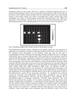
Why is Fatigue Resistance so Good?
Paradox: Glass is a very brittle material (no plastic deformation). The resin is also
often a brittle material. (for example, epoxy). However, the association of reinforce-
ment/matrix constituted of these two materials opposes to the propagation of cracks
and makes the resultant composite to endure fatigue remarkably.
Explanation: When the cracks propagate, for example, in the unidirectional
layer shown schematically in Figure 5.30 in the form of alternating of fibers and
Figure 5.28b Three Plies, Together
Figure 5.28c Stresses at Free Edge
TX846_Frame_C05 Page 111 Monday, November 18, 2002 12:09 PM
© 2003 by CRC Press LLC