Heat and Mass Transfer Modeling and Simulation Part 4 docx

Numerical Analysis of Heat and Mass Transfer in a Fin-and-Tube
Air Heat Exchanger under Full and Partial Dehumidification Conditions
51
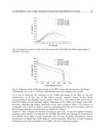
The distributions of these velocities over the physical domain, where the half fin length and
high are settled to 2.5, are shown in Fig. 6a and 6b.


Fig. 6a. Horizontal velocity distribution


Fig. 6b. Vertical velocity distribution
-2.5 -2 -1.5 -1 -0.5 0 0.5 1 1. 5 2 2.5
-2.5
-2
-1.5
-1
-0.5
0
0.5
1
1.5
2
2.5
0
.
2
0
.
2
0.2
0

.
2
0.4
0
.
4
0
.
4
0
.
4
0.6
0
.
6
0
.
6
0
.
6
0
.
6
0
.
8
0
.

8
0
.
8
0
.
8
0.8
0.8
0.
8
1
1
1
1
1
1
1
1
1
.
2
1
.
2
1
.
2
1
.

2
1
.
2
1
.
2
1
.
4
1
.
4
1
.
4
1
.
4
1
.
6
1
.
6
x*
y*

-2.5 -2 -1.5 -1 -0.5 0 0.5 1 1. 5 2 2.5
-2.5

-2
-1.5
-1
-0.5
0
0.5
1
1.5
2
2.5
-
0
.
6
-
0
.
6
-
0
.
4
-0
.
4
-
0
.
4
-

0
.
4
-
0
.
2
-
0
.
2
-
0
.
2
-
0
.
2
-
0
.
2
-
0
.
2
0
0
0

0
0
0
0
.
2
0
.
2
0
.
2
0
.
2
0
.
2
0
.
2
0
.
4
0
.
4
0
.
4

0
.
4
0
.
6
0
.
6
y*
x*
air
air

Heat and Mass Transfer – Modeling and Simulation
52
As shown in Fig. 6a and 6b, the horizontal and vertical velocities fields present an apparent
symmetry regarding x and y axes. The horizontal dimensionless velocity at the inlet and
outlet tends towards unity, is maximal at the upper and lower fin edges and is minimal
close to the tube wall as a result of the channel reduction. Likewise, the vertical
dimensionless velocity is close to zero when going up the inlet and outlet or the upper and
lower fin edges, and is also minimal near the tube surface.
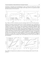
2.4.2 Solving heat and mass transfer equations
The heat and mass transfer problem has been solved using an appropriate meshing of the
calculation domain and a finite-volume discretization method. Fig. 7 illustrates the fin
meshing configuration used.

-2.5 -2 -1.5 -1 -0.5 0 0.5 1 1.5 2 2.5
2.5
2
1.5
1
0.5
0
-0.5
-1
-1.5
-2
-2.5



Fig. 7. Fin meshing with 627 nodes. (h
*
=2.5, l
*
=2.5)
In this work, up to 11785 nodes are used in order to take into account the effect of the
mesh finesse on the process convergence and results reliability. The deviations on the
calculation results of the fin efficiency with the different meshing prove to be less than 0.3
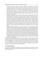
%. The numerical simulation is achieved using MATLAB simulation software. A global
calculation algorithm for heat and mass transfer models is developed and presented in
Fig. 8.
Numerical Analysis of Heat and Mass Transfer in a Fin-and-Tube
Air Heat Exchanger under Full and Partial Dehumidification Conditions
53

Fig. 8. The global calculation algorithm for heat and mass transfer models
Identify the fin temperature (eq. 41)
Calculate air local velocity (eqs. 45 and 46)
Calculate local sensible heat transfer coefficient (eq. 60)
Calculate T
a
and W
a
(eqs. 30 and 25)
Calculate the condensate-film thickness (53)
no
yes
Condensate flow rate (3), heat flow rate (5),fin efficiency (67)
Calculate the boundary-layer thickness (eq. 59)
Input parameters: u
i
, RH
i
, T
a,i
, T
f,b
, p
f
, l, h, Le
Initialization of variables: T
a
, RH, 
c

Calculate proprerties (ρ, μ, ν, λ, L
v
, c
p
)
Calculate local overall heat transfer coefficient (7)




?10
6
1
,, 


N
ji
a
N
ji
a
TT




?10
6
1

,, 


N
ji
f
N
ji
f
TT




?10
6
1
,, 


N
ji
a
N
ji
a
WW
Identify the fin temperature (eq. 41)
Calculate air local velocity (eqs. 45 and 46)
Calculate local sensible heat transfer coefficient (eq. 60)

Calculate T
a
and W
a
(eqs. 30 and 25)
Calculate the condensate-film thickness (53)
no
yes
Condensate flow rate (3), heat flow rate (5),fin efficiency (67)
Calculate the boundary-layer thickness (eq. 59)
Input parameters: u
i
, RH
i
, T
a,i
, T
f,b
, p
f
, l, h, Le
Initialization of variables: T
a
, RH, 
c
Calculate proprerties (ρ, μ, ν, λ, L
v
, c
p
)

Calculate local overall heat transfer coefficient (7)




?10
6
1
,, 


N
ji
a
N
ji
a
TT




?10
6
1
,, 


N
ji

f
N
ji
f
TT




?10
6
1
,, 


N
ji
a
N
ji
a
WW

Heat and Mass Transfer – Modeling and Simulation
54
2.5 Heat performance characterization
In order to evaluate the fin thermal characteristics, we need to define the heat transfer
coefficients, the Colburn factor j, and the fin efficiency

f

.
2.5.1 Colburn factor
The sensible Colburn factor is expressed as:

1/3
Re .Pr
sen
sen
Dh
Nu
j

(47)
The Reynolds number based on the hydraulic diameter is defined as follows:

max,
Re
aah
Dh
a
uD



(48)
where the maximal moist air velocity
max,a
u
is obtained at the contraction section of the
flow :

*
max,
*
2
22
ai
h
uu
h


(49)
By definition, the hydraulic diameter is expressed as:

** * *
** *
82
4
h
hlp p
D
hl p






(50)

The Nusselt and Prandtl numbers are given by:

,
.
sen hum h
sen
a
D
Nu



(51)

,
.
Pr
a
p
a
a
c



(52)
The Colburn factor takes into account the effect of the air speed and the fin geometry in the
heat exchanger. Knowing the heat transfer coefficient, the determination of Colburn factor
becomes usual.
2.5.2 Heat transfer coefficients

Regarding the physical configuration of the fin-and-tube heat exchanger, the condensate
distribution over the fin-and-tube is complex. In this work, the condensate film is assumed
uniformly distributed over the fin surface and the effect of the presence of the tube on the
film distribution is neglected. The average condensate-film thickness is calculated as follow:

ft
t
AA
c
A
c
f
ds
A





(53)
Numerical Analysis of Heat and Mass Transfer in a Fin-and-Tube
Air Heat Exchanger under Full and Partial Dehumidification Conditions
55
where A
f
denotes the net fin area:

2
4
f

A
lh r


(54)
And A
t
represents the total tube cross section:

2
t
A
r

 (55)
The condensate-thickness 
c
is calculated using equation (37) and can be estimated
iteratively. Assuming the temperature profile of the condensate-film to be linear, the heat
transfer coefficient of condensation is obtained as follow:

c
c
c




(56)
The theory of hydrodynamic flow over a rectangular plate associated with heat and mass

transfer allows us to evaluate the sensible heat transfer coefficient. In this case, a hydro-
thermal boundary-layer is formed and results from a non-uniform distribution of
temperatures, air velocity and water concentrations across the boundary layer (Fig.9).


Fig. 9. Thermal and hydrodynamic boundary layer on a plate fin
According to Blasius theory, the hydraulic boundary layer thickness can be defined as
follow:

1/2
5.
Re
H
L
x

 with
.
Re
a
L
a
ux


(57)
where Re
L
is the Reynolds number based on the longitudinal distance x.
By analogy, the thermal boundary layer thickness is associated to the hydraulic boundary

layer thickness through the Prandtl number (Hsu, 1963):

1/3
Pr
T
H




(58)
The expression of 
t
takes the following form:
Moist air
(T
a,i
, W
a,i
, u
i
)
air (T
a
, W
a
, u
a
)
Fcondensate-film

(T
c
, W
S,c
)
fin
Thermal
boundary
layer
Hydrodynamic
boundary layer
u(δ)=u
a
T(δ)=T
a
x0
z
Moist air
(T
a,i
, W
a,i
, u
i
)
Moist air
(T
a,i
, W
a,i

, u
i
)
air (T
a
, W
a
, u
a
)
Fcondensate-film
(T
c
, W
S,c
)
fin
Thermal
boundary
layer
Hydrodynamic
boundary layer
u(δ)=u
a
T(δ)=T
a
x0
z
x0
z

Heat and Mass Transfer – Modeling and Simulation
56

1/2 1/3
5.
Re .Pr
T
L
x


(59)
Assuming a linear profile of temperature along within the boundary layer, the sensible heat
transfer coefficient is related to the thermal boundary layer thickness by the following relation:

,
a
sen hum
T




(60)
Where, 
t
is the average thickness of the thermal boundary layer.
The overall heat transfer coefficient, estimated from equation (7), involves the sensible heat-
transfer coefficient and the part due to mass transfer. The exact values of the average

sensible and overall heat-transfer coefficients can be obtained by:

,
,
ft
t
AA
sen hum
A
sen hum
f
ds
A






,
,
ft
t
AA
Ohum
A
Ohum
f
ds
A






(61)
2.5.3 Fin efficiency
In this work, the local fin efficiency in both dry and wet conditions is estimated by the
following relations:




,
**
,
,,,
sen dry a f
fdry a f
sen dry a i f b
TT
TT
TT








(62)




,
,
2/3 2/3
,,
**
,
,,,
,,,
2/3 2/3
,,
,,
1. 1.
1. 1.
aSf
sen hum a f
af
pa pa
fhum af
ai S f b
sen hum a i
f
b i
ai fb
pa pa
WW

Lv Lv
TT C
TT
Le c Le c
TT
WW
Lv Lv
TT C
TT
Le c Le c






 







 



(63)
Where the condensation factors are given by:

,aS
f
af
WW
C
TT



(64)

,,,
,,
ai S
f
b
i
ai f b
WW
C
TT



(65)
The averages values of the fin efficiencies over the whole fin are estimated as follow:


**

,
,
,
ft
t
ft
t
AA
sen dry a f
A
fdry
AA
sen dry
A
TTds
ds









(66)
Numerical Analysis of Heat and Mass Transfer in a Fin-and-Tube
Air Heat Exchanger under Full and Partial Dehumidification Conditions
57


**
,
2/3
,
,
,
2/3
,
1.
1.
ft
t
ft
t
AA
sen dry a f
pa
A
fhum
AA
i sen dry
pa
A
Lv
TT Cds
Le c
Lv
Cds
Le c



















(67)
3. Results and discussion
In This section, the simulation results of the heat and mass transfer characteristics during a
streamline moist air through a rectangular fin-and-tube will be shown. The effect of the
hydro-thermal parameters such us air dry temperature, fin base temperature, humidity, and
air velocity will be analyzed. The key-parameters values for this work are selected and
reported in the table 1. A central point is uncovered for the main results representations.
This point corresponds to a fully wet condition problem.

Parameter Central point values range
Fin hi
g

h, h
*
2.5 -
Fin len
g
th, l
*
2.5 -
Fin s
p
acin
g
,
p
*
0.16 -
Inlet air s
p
eed, u
i
3 m/s 1-5 m/s
Fin base tem
p
erature,
T
f
,b
9 °C 1-9 °C
Inlet air dr
y

tem
p
erature,
T
a,i
27 °C 24-37 °C
Inlet air relative humidit
y
, R
H
i
50 % 20-100 %
Lewis number, Le 1-
Table 1. Values of the parameters used in this work
3.1 The fully wet condition
Figures 10a and 10b show, respectively, the distribution of the curve-fitted air temperature
inside the airflow region and that of the fin temperature for the values of the parameters
indicated by the central point.


Fig. 10a. Air temperature distribution
-2.5 -2 -1.5 -1 -0.5 0 0.5 1 1.5 2 2.5
-2.5
-2
-1.5
-1
-0.5
0
0.5
1

1.5
2
2.5
0
.
9
7
0
.
9
7
0
.
9
4
0
.
9
1
0
.
9
1
0
.
8
8
0
.
8

8
0
.
9
4
y*
x*
-2.5 -2 -1.5 -1 -0.5 0 0.5 1 1.5 2 2.5
-2.5
-2
-1.5
-1
-0.5
0
0.5
1
1.5
2
2.5
0
.
9
7
0
.
9
7
0
.
9

4
0
.
9
1
0
.
9
1
0
.
8
8
0
.
8
8
0
.
9
4
y*
x*

Heat and Mass Transfer – Modeling and Simulation
58

Fig. 10b. Fin temperature distribution
Initially, the air temperature is uniform (T
*

a
=1) then decreases along the fin. As the fin
temperature is minimal at the vicinity of the tube, air temperature gradient is more
important near the tube than by the fin borders. However, at the outlet of the flow, the
temperature gradient of air is weaker than at the inlet due to the reduction of the sensible
heat transfer upstream the fin. The increasing of the boundary layer thickness along the fin
causes a drop of the heat transfer coefficient. It is worth noting that the isothermal
temperature curves are normal to the fin borders because of the symmetric boundary
condition. Concerning the fin temperature T
*
f
, it decreases from the inlet to attain a
minimum nearby the fin base surface and then increases again when going away the tube.
For this case of calculation, the dew point temperature of air, corresponding to HR
i
=50 %
and T
a,i
=27 °C, is equal to 16.1 °C, that is greater than the maximal temperature of the fin
(13.4 °C) and the fin will be completely wet. The condensation factor C, defined by equation
(64), allows us to verify this fact. Fig. 11 illustrates its distribution over the fin region.


Fig. 11. Condensation factor distribution
-2.5 -2 -1.5 -1 -0.5 0 0.5 1 1.5 2 2.5
-2.5
-2
-1.5
-1
-0.5

0
0.5
1
1.5
2
2.5
0
0
.
0
5
0.05
0
.
0
5
0
.
0
5
0
.
0
5
0
.
1
0
.
1

0
.
1
0
.
1
0
.
1
0
.
1
0
.
1
5
0
.
1
5
0
.
1
5
0
.
1
5
0
.

1
5
0
.
1
5
0
.
1
5
0
.
2
0
.
2
0
.
2
0
.
2
0
0
0
y*
x*
-2.5 -2 -1.5 -1 -0.5 0 0.5 1 1.5 2 2.5
-2.5
-2

-1.5
-1
-0.5
0
0.5
1
1.5
2
2.5
0
0
.
0
5
0.05
0
.
0
5
0
.
0
5
0
.
0
5
0
.
1

0
.
1
0
.
1
0
.
1
0
.
1
0
.
1
0
.
1
5
0
.
1
5
0
.
1
5
0
.
1

5
0
.
1
5
0
.
1
5
0
.
1
5
0
.
2
0
.
2
0
.
2
0
.
2
0
0
0
y*
x*

-2.5 -2 -1.5 -1 -0.5 0 0.5 1 1.5 2 2.5
-2.5
-2
-1.5
-1
-0.5
0
0.5
1
1.5
2
2.5
0
.
1
4
0
.
1
4
0
.
1
4
0
.
1
4
0
.

1
6
0.16
0
.
1
6
0
.
1
6
0
.
16
0
.
1
6
0
.
1
6
0
.
1
6
0
.
1
8

0
.
1
8
0
.
1
8
0
.
1
8
0
.
1
8
0
.
1
8
0
.
2
0
.
2
0
.
2
0

.
2
0
.
2
0
.
2
2
0
.
2
2
0
.
2
2
0
.
2
2
0
.
2
2
y*
x*
-2.5 -2 -1.5 -1 -0.5 0 0.5 1 1.5 2 2.5
-2.5
-2

-1.5
-1
-0.5
0
0.5
1
1.5
2
2.5
0
.
1
4
0
.
1
4
0
.
1
4
0
.
1
4
0
.
1
6
0.16

0
.
1
6
0
.
1
6
0
.
16
0
.
1
6
0
.
1
6
0
.
1
6
0
.
1
8
0
.
1

8
0
.
1
8
0
.
1
8
0
.
1
8
0
.
1
8
0
.
2
0
.
2
0
.
2
0
.
2
0

.
2
0
.
2
2
0
.
2
2
0
.
2
2
0
.
2
2
0
.
2
2
y*
x*
Numerical Analysis of Heat and Mass Transfer in a Fin-and-Tube
Air Heat Exchanger under Full and Partial Dehumidification Conditions
59
As can be observed from Fig. 11, the condensation factor takes the largest values in the
vicinity of the tube wall. The difference between the maximal and minimal values is about
30 %. The variation of C against the fin base temperature T

f
and relative humidity HR can be
demonstrated by the subsequent reasoning. The saturation humidity ratio of air may be
approximated by a second order polynomial with respect to the temperature (Coney et al.,
1989, Chen, 1991):

2
S
WabTcT 
(68)
Where a,b and c are positives constants
The relative humidity has the following expression:

,,
vaav
av SaaSv
PWPP
RH
PP W PP



(69)
Where P
a
, P
v
and P
s,v
respectively represent, air total pressure, water vapor partial pressure

and water vapor saturation pressure. If we neglect the water vapor partial and saturation
pressures regarding the total pressure, then the following expressions of the absolute
humidity arise:

,aSa
WRHW
(70)

,,,ai Sai
WRHW
(71)
Substituting equations (68) to (71) into the relation defining C (Eq. 64) yields:



2
1
ff
af
af
abT cT
CRH bcT T RH
TT


  


(72)
The first and second order derivatives of the condensation factor with respect to the fin

temperature can then be obtained readily from the previous equation:



,
2
1
Sa
f
RH
af
W
C
RH c RH c
T
TT






  









(73)



2
,
23
2
1
Sa
f
af
RH
W
C
RH
T
TT





 









(74)
Obviously, for saturated air stream (RH=1), the first derivative of C takes the value of the
constant c and is consequently positive. That demonstrates the increase of the condensation
factor C with the fin temperature T
f
. Conversely, for a sub-saturated air (RH<1), the second
order derivative is always negative, that implies a permanent decrease of the condensation
factor gradient with temperature. In this case, the critical point (maximum) for the function
C(Tf) can be evaluated when
0
f
RH
C
T



, thus, we obtain:

Heat and Mass Transfer – Modeling and Simulation
60


,,
1./
fcr a Sa
TT RHWc 

(75)
or


2
,
1
af
cr
Sa
cT T
RH
W


(76)
Therefore the following statement is deduced:
-
When T
f
> T
f,cr
or RH < RH
cr
, then (C/T
f
)
RH
< 0 and C decreases with T
f

.
-
When T
f
< T
f,cr
or RH > RH
cr
, then (C/T
f
)
RH
> 0 and C increases with T
f
.
Fig. 11 is consistent with the above statement. Indeed, we can observe from Fig.10b and
Fig.11 that the local condensation factor decreases with the fin temperature. Also, for the
conditions in which the calculation related to Fig.10b and Fig.1 was performed, we get
c=9.3458x10-6 and W
S,a
=0.0202, hence, from Eqs. (75) and (76), T
f,cr
=-6°C and RH
cr
=90 %.
Since Fig. 12 shows that T
f
> T
f,b
> T

f,cr
, this observation validates our statement. However, it
is also worth noting that the relative humidity of the moist air varies with the fin
temperature and as a matter of fact, RH should be temperature dependent and the above
statements hold along a constant relative humidity curve. Fig. 12 represents the distribution
of air relative humidity in the fin region.


Fig. 12. Relative humidity distribution
As can be observed in Fig. 12, the relative humidity evolves almost linearly along the fin
length. There is about 13 % difference between the inlet and outlet airflow.
Correspondingly, the distribution of the condensate mass flux and the total heat flux density
are carried out and illustrated in Fig. 13 and 14.
As the condensation factor takes place at the surrounding of the tube where the maximum
gradient of humidity occurs, the condensate mass flux m
”
c
gets its maximal value at the fin
base. Similarly, the maximal temperature gradient (T
a
-T
f
) arises at the fin base. That
enhances the heat flow rate and a maximal value of q
”
t
is reached. However, these quantities
decrease more and more along the dehumidification process due to the humidity and
temperature gradients drop. Further results are shown in Fig.15, where the fin efficiency
-2.5 -2 -1.5 -1 -0.5 0 0.5 1 1.5 2 2.5

-2.5
-2
-1.5
-1
-0.5
0
0.5
1
1.5
2
2.5
0
.
5
1
0.51
0.51
0
.
5
2
0.52
0.52
0
.
5
3
0
.
5

4
0
.
5
4
0
.
5
5
0
.
5
5
0
.
5
6
0
.
5
6
0
.
5
6
y*
x*
0
.
5

3
-2.5 -2 -1.5 -1 -0.5 0 0.5 1 1.5 2 2.5
-2.5
-2
-1.5
-1
-0.5
0
0.5
1
1.5
2
2.5
0
.
5
1
0.51
0.51
0
.
5
2
0.52
0.52
0
.
5
3
0

.
5
4
0
.
5
4
0
.
5
5
0
.
5
5
0
.
5
6
0
.
5
6
0
.
5
6
y*
x*
0

.
5
3
Numerical Analysis of Heat and Mass Transfer in a Fin-and-Tube
Air Heat Exchanger under Full and Partial Dehumidification Conditions
61
curves are plotted. As the condensation factor C and the difference (T
a
* - T
f
*) grow around
the tube, the fin efficiency will be maximal at the centre. As well, the quantities C and (T
a
* -
T
f
*) are weaker at the upper and lower fin borders, that leads to the local reduction of the fin
efficiency.


Fig. 13. Condensate mass flux distribution


Fig. 14. Heat flux density distribution
3.2 The partially wet condition
The partially wet fin is obtained when the initial conditions are fixed to those of the central
point (Table 1) except the inlet relative humidity which is settled to RH = 36 %, since
T
f,b
<T

dew,a
< T
f,max
. Condensation factor, relative humidity, total heat flux, and fin efficiency
are estimated. The same general observations as those of the fully wet fin can be
withdrawn. Condensation factor, total heat flux density and fin efficiency are maximal at the
fin tube. However, the condensate droplets come to the end (C=0) from certain distance of
the tube. At this point, the effect of some parameters, like inlet temperature, on the heat and
mass transfer characteristics will be presented and discussed.
-2.5 -2 -1.5 -1 -0.5 0 0.5 1 1.5 2 2.5
-2.5
-2
-1.5
-1
-0.5
0
0.5
1
1.5
2
2.5
0
.
0
4
0
.
0
4
0

.
0
5
0
.
0
5
0
.
0
5
0
.
0
5
0
.
0
5
0
.
0
5
0
.
0
5
0
.
0

6
0
.
0
6
0
.
0
6
0
.
0
6
0
.
0
6
0
.
0
6
0
.
0
7
0
.
0
7
0

.
0
7
0
.
0
7
0
.
0
7
0
.
0
8
0
.
0
8
0
.
0
8
0
.
0
8
y*
x*
-2.5 -2 -1.5 -1 -0.5 0 0.5 1 1.5 2 2.5

-2.5
-2
-1.5
-1
-0.5
0
0.5
1
1.5
2
2.5
0
.
0
4
0
.
0
4
0
.
0
5
0
.
0
5
0
.
0

5
0
.
0
5
0
.
0
5
0
.
0
5
0
.
0
5
0
.
0
6
0
.
0
6
0
.
0
6
0

.
0
6
0
.
0
6
0
.
0
6
0
.
0
7
0
.
0
7
0
.
0
7
0
.
0
7
0
.
0

7
0
.
0
8
0
.
0
8
0
.
0
8
0
.
0
8
y*
x*
-2.5 -2 -1.5 -1 -0.5 0 0.5 1 1.5 2 2.5
-2.5
-2
-1.5
-1
-0.5
0
0.5
1
1.5
2

2.5
4
0
0
4
0
0
4
0
0
4
5
0
4
5
0
45
0
4
5
0
4
5
0
4
5
0
4
5
0

5
0
0
5
0
0
5
0
0
5
0
0
5
0
0
550
5
5
0
6
0
0
6
0
0
6
0
0
5
5

0
5
5
0
5
5
0
y*
x*
6
0
0
-2.5 -2 -1.5 -1 -0.5 0 0.5 1 1.5 2 2.5
-2.5
-2
-1.5
-1
-0.5
0
0.5
1
1.5
2
2.5
4
0
0
4
0
0

4
0
0
4
5
0
4
5
0
45
0
4
5
0
4
5
0
4
5
0
4
5
0
5
0
0
5
0
0
5

0
0
5
0
0
5
0
0
550
5
5
0
6
0
0
6
0
0
6
0
0
5
5
0
5
5
0
5
5
0

y*
x*
6
0
0

Heat and Mass Transfer – Modeling and Simulation
62
3.3 Effect of the inlet relative humidity
Both ideal and real fins are considered, and it is observed that 
c
starts to increase rapidly at
about RH
i
=40 %. For this case, the dry fin limit is estimated at RH
i
=32 % and the fully wet
condition beginning is estimated at RH
i
=42 %. The order of magnitude of 
c
is about 0.1 mm,
this value is comparable to that of Myers (1967) (0.127 mm) for, approximately, the same
conditions. As 
c
increase with RH
i
, the thermal resistance of the condensate increases and
the heat transfer coefficient of the condensate 
c

decreases (Eq.56). This agrees with the
result of Coney et al. [10]. It was found also that the sensible heat transfer coefficient 
sen,hum

is insensitive to RH
i
(Fig. 21). Due to the smallness of the condensate film thickness, its
thermal resistance (1/
c
) is in the order of 0 to 5 % regarding the thermal resistance of the
surrounding air. It is usually neglected. Conversely, the average overall heat transfer
coefficient increases rapidly as the relative humidity increases. For a dry fin (RH
i
<32 %), the
total heat amount of both ideal and real fins is constant and consequently the fin efficiency
remains constant in this range. The condensation appears from RHi=32 % for an ideal fin
and from RH
i
=36 % for a real fin. At this range (32%<RH
i
<36%), the relative difference
between ideal and real heats {(Q
t,id
-Q
t,r
)/Q
i,id
} is important, thus an abrupt decrease in fin
efficiency is noticed. For RH
i

=36 %, the condensation begins on the real fin and the total heat
exchange rate Q
t,r
increases, thus the relative difference between ideal and real heats
exchanges rates become less important and narrows more and more, therefore, the decrease
in fin efficiency is gradual with a slop around 8 %. At RH
i
=42 %, a complete wet condition is
achieved for the real fin, the relative difference between Q
t,r
and Q
t,id
is almost constant. As
well, the fin efficiency reduces slightly with a slop less than 4 %. Hence, the condensation,
enhanced by increasing the relative humidity, can affect the efficiency and reduces it by 12
%. The fin efficiency gradient regarding relative humidity RH
i
in the partial wet condition is
more important than in the fully wet condition. The efficiency decreases more quickly in the
partial wet condition. This result is similar of those of Rosario & Rahman (1999), Wu & Bong
(1999), Liang et al. (2000), and Threlkeld (1970). However, Hong & Webb (1996), Elmahdy &
Biggs (1983), and Mc Quiston (1975) have observed a more important decrease of the fin
efficiency in the complete humidified phase (until 35 %). But, their models assume a
constant temperature and relative humidity of the surrounding air. Kandlikar (1990) has re-
examined the mathematical model of Elmahdy & Biggs (1983) and demonstrates that the fin
efficiency in the fully wet condition should be insensitive to the relative humidity. It can be
demonstrated that the results found by Hong & Webb (1996), and Mc Quiston (1975) are the
consequence of the assumptions undertaken in their models. Indeed, if we consider again
the expression of the fin efficiency in humid conditions (Eq. 67):





**
,
1.
1.
fhum a f
i
C
TT
C






(77)
where;
2/3
,
p
a
Lv
Le c

 and
,,,

,,
ai S
f
b
i
ai f b
WW
C
TT




Assuming Ta and C to be constant, as in the models of Hong & Webb (1996) and Mc Quiston
(1975), the derivation of equation (77) with respect to RH
i
yields:
Numerical Analysis of Heat and Mass Transfer in a Fin-and-Tube
Air Heat Exchanger under Full and Partial Dehumidification Conditions
63



*
,,,,
,,

1.
fhum f fhum Sai
ii

ai
f
bi
TW
RH RH
TT C



 


(78)
Performing calculations of the fin efficiency derivative at 
f,hum
=0.7 and using the
parameters mentioned in figure 25, T
a,i
=27 °C, T
f,b
=9 °C, the following results yields:
*
0.3
f
i
T
RH




;
,
1.1
fhum
i
RH





for RH
i
=50 %
and
,
0.42
fhum
i
RH




for RH
i
=100 %
The decrease of the fin efficiency gradient between RH
i
=50 % and RH

i
=100 % is about 21 %.
Therefore, the discordance founded between the different authors about the effect of the
relative humidity on the fin efficiency may be the result of the models simplifications adopted.
3.4 Effect of the inlet air temperature
For a fixed RH
i
, the increase of the inlet air temperature T
a,I
leads to increasing both fin and
airflow temperatures (T
f
and T
a
). Thus, it has been noticed that the variations of the
dimensionless fin and air temperatures are insignificant. However, the absolute moist air
humidity raises and generates a more important humidity gradient between the fin wall and
the surrounding air, and hence contributes to increase the condensation factor. Indeed, the
derivation of C (Eq. 64) with respect to air temperature yields a positive derivative:

,
.(1). 0
Sf
aaf
RH
W
C
cRH RH
TTT



 

(79)
As the absolute humidity increase with T
a,I
, the mass transfer is enhanced and the
condensate-film thickness also increases. On the other hand, the increase of W
a,i
and W
a

results in raising the condensation factor C and the latent heat rate, and that makes the
overall heat transfer coefficient more important for a greater temperatures. Nonetheless, in
the absence of condensation (RH
i
from 0 to about 32 %), the overall and sensible heat
transfer coefficients are equivalent and independent of the air temperature. With increasing
air temperature, the total heat rate increases and the condensation starts for lower values of
RH
i
. The vapor condensation appearance is distinguished from RH
i
=26 % (ideal fin) or
RH
i
=32 % (real fin) for T
a,i
=30 °C and from RH
i

=38 % (ideal fin) or RH
i
=44 % (real fin) for
T
a,i
=24 °C. In the dry phase, the heat rate remains constant which implies a constancy of fin
efficiency. At this stage, the fin efficiency decreases slightly with the increasing of air
temperature. When condensation begins, the total heat rate increases with RHi and an
abrupt decrease of fin efficiency is observed. This drop in the fin efficiency is slightly weak
for greater air temperatures. In the fully wet condition and for higher relative humidity
values, the fin efficiency decreases distinctly when Ta,I increase. These observations match
with those reported by Kazeminejad (1995) and Rosario & Rahman (1999).
3.5 Effect of the fin base temperature
As stated above (Eq. 64), the dependence of C on the fin temperature T
f
is marked with the
existence of a critical value of RH
i
where the trend progression is inverted. That is clearly

Heat and Mass Transfer – Modeling and Simulation
64
observed in Fig.30. For RH
i
<RH
cr
, the condensation factor decreases with the fin base
temperature, whereas, for RH
i
>RH

cr
, C increases with T
f,b
. Correspondingly, the trend of C
is also inverted depending on whether the fin is real or ideal. Indeed, the ideal C factor is
higher than the real C for RH
i
< RH
cr
, while it is lower for RH
i
> RH
cr
. As the absolute
humidity near the fin wall W
S,f,b
increases with T
f,b
, the amount of condensable vapor
decreases, which in turn causes the reduction of the average condensate-film thickness as
illustrated in Fig.31. However, the overall heat transfer coefficient follows the same trend as
the condensation factor. For the dry condition, the sensible heat transfer is independent on
T
f,b
. Conversely, for the humid condition, 
t,hum
decreases with T
f,b
when RH
i

< RH
cr
and
increases with Tf,b when RH
i
> RH
cr
. It is worth noting that since 
t,hum
is influenced by the
boundary layer thickness, the critical relative humidity RH
cr
for which the trend of 
t,hum

changes is to some extent different from the critical value obtained with C. In our case, 
t,hum

begins to increase with T
f,b
from RH
i
=85 % instead of RH
i
=78 % as regards to C. The increase
of T
f,b
leads an increase of W
S,f,b
and thus reduces both the total heat rate and the fin

efficiency. In the partially humid condition case, a rapid drop of 
f
is confirmed (about 10
%). This drop proves to be smaller for the fully wet condition (about 2%). Nevertheless, the
variation of T
f,b
has no significant effect on the fin efficiency for the dry condition. Our
results concerning the fin efficiency behavior with regard to the fin temperature agree with
those of Rosario & Rahman (1999) but prove to be dissimilar from those established by
Kazeminejad (1995). This is probably due to the fact that Rosario & Rahman consider the
condensation factor to be variable while Kazeminejad assumes it as constant.
3.6 Effect of the inlet air speed
Increasing u
i
reduces the hydro-thermal boundary layer thickness and increases the heat
transfer coefficient. The temperature of air in the flow core also increases since the flow mass
increases more rapidly than the heat flow rate, thus the fin temperature will be more
important. Furthermore, as the air mass flow rate increases more rapidly than the
condensate mass flow rate, the difference between airflow humidity and the saturated air
humidity at the fin neighborhood (W
a
– W
S,f
) increases. That means an increase in the
condensation factor as well as in the condensate thickness. In the same way, as the hydro-
thermal boundary layer becomes finer for higher flow regime, the sensible heat transfer is
favored. Thus, the sensible and overall heat transfer coefficients increase with u
i
. However,
this increase narrows down for highest air speed. On the other hand, the influence of u

i
on
the heat transfer is such as the total heat rate increase with increasing the flow regime. In the
case of an ideal fin, the heat transfer increasing is quicker than for a real fin. This result has
also been demonstrated numerically by Coney et al. (1989). Accounting for that effect, the fin
efficiency should decrease with u
i
, as mentioned in Fig. 36. Indeed, for lower velocities ui,
the residence time of air is more important and the heat and mass transfer is more complete.
This result is in adequacy with those of Liang et al. (2000) and Coney et al. (1989). Moreover,
it is found that the difference between dry and humid fin efficiencies (
f,dry
- 
f,hum
) increases
with u
i
.
4. Conclusions
The present work proposes a two-dimensional model simulating the heat and mass transfer
in a plate fin-and-tube heat exchanger. Ones the airflow profile was determined, the water
vapor, air stream and fin heat and mass balance equations were solved simultaneously. It
Numerical Analysis of Heat and Mass Transfer in a Fin-and-Tube
Air Heat Exchanger under Full and Partial Dehumidification Conditions
65
was found that the overall heat transfer coefficient as well as the condensation factor
increase with the inlet air temperature, the inlet relative humidity as well as the inlet
velocity. Regarding the variations of 
t,hum
and C with the fin base temperature, a critical

value of relative humidity (RH
cr
), corresponding to a minimum in 
t,hum
and C was
identified. This result still constitutes a point of discordance between many authors. The
performed calculations of the wet-fin efficiency have demonstrated the decrease of 
f,hum
with increasing any of the parameters. However, a more important drop of 
f,hum
have been
noticed for the partially wet condition. Moreover, the decrease of the fin efficiency with
respect to the relative humidity and the fin base temperature, in the fully wet condition, is
very weak especially for higher values of RH
i
or T
f,b
. The slope is quantified around 2 %.
5. References
Benelmir, R.; Mokraoui, S.; Souayed, A. (2009). Numerical analysis of filmwise condensation
in a plate fin-and-tube heat exchanger in presence of non condensable gas, Heat
and Mass Transfer Journal, 45, 1561–1573.
Chen, L.T. (1991). Two-dimensional fin efficiency with combined heat and mass transfer
between water-wetted fin surface and moving moist airstreams, Int. J. Heat Fluid
Flow, 12, 71-76.
Chen, H.T.; Song, J.P.; Wang, Y.T. (2005). Prediction of heat transfer coefficient on the fin
inside one-tube plate finned-tube heat exchangers, Int. J. Heat Mass Transfer, 48,
2697-2707.
Chen, H.T. ; Wang, Y.T. (2008). Estimation of heat-transfer characteristics on a fin under wet
conditions, Int. J. Heat Mass Transfer, 51, 2123-2138.

Chen, H.T.; Hsu, W.L. (2007). Estimation of heat transfer coefficient on the fin of annular-
finned tube heat exchangers in natural convection for various fin spacings, Int. J.
Heat Mass Transfer, 50, 1750-1761.
Chen, H.T.; Chou, J.C. (2007). Estimation of heat transfer coefficient on the vertical plate fin
of finned-tube heat exchangers for various air speeds and fin spacings, Int. J. Heat
Mass Transfer, 50, 47-57.
Choukairy, Kh. ; Bennacer, R. ; El Ganaoui, M. (2006). Transient behaviours inside a vertical
cylindrical enclosure heated from the sidewalls, Num. Heat Transfer (NHT), 50-8,
773 – 785.
Coney, J.E.R. ; Sheppard, C.G.W. ; El-Shafei, E.A.M. (1989). Fin performance with
condensation from humid air, Int. J. Heat Fluid Flow, 10, 224-231.
Elmahdy, A.H. ; Biggs, R.C. (1983). Efficiency of extended surfaces with simultaneous heat
transfer and mass transfer, ASHRAE Journal, 89-1A, 135-143.
Hong, T.K. ; Webb, R.L. (1996). Calculation of fin efficiency for wet and dry fins, HVAC &
Research, 2-1, 27-41.
Hsu, S.T. (1963). Enginnering heat transfer, D. VanNostrand Company, 240-252.
Johnson, R.W. (1998). The Handbook of Fluid Dynamics, Springer, USA.
Kandlikar, S.G. (1990). Thermal design theory for compact evaporators, Hemisphere
Publishing, NY, pp. 245-286.
Kazeminejad, H. (1995). Analysis of one-dimensional fin assembly heat transfer with
dehumidification, Int. J. of Heat mass transfer, 38-3, 455-462.

Heat and Mass Transfer – Modeling and Simulation
66
Khalfi, M.S. ; Benelmir, R. (2001). Experimental study of a cooling coil with wet surface
conditions, Int. Journal of Thermal Sciences, 40, 42-51.
Lin, C.N.; Jang, J.Y. (2002). A two-dimensional fin efficiency analysis of combined heat and
mass transfer in elliptic fins, Int. J. Heat Mass Transfer, 45, 3839-3847.
Lin, Y.T. ; Hsu, K.C. ; Chang, Y.J. ; Wang, C.C. (2001). Performance of rectangular fin in wet
conditions: visualization and wet fin efficiency, ASME J. Heat Transfer, 123, 827-

836.
Liang, S.Y.; Wong, T.N.; Nathan, G.K. (2000). Comparison of one-dimensional and two-
dimensional models for wet-surface fin efficiency of a plate-fin-tube heat
exchanger, Appl. Thermal Eng, 20, 941-962.
McQuiston, F.C. (1975). Fin efficiency with combined heat and mass transfer, ASHRAE
Journal, 81, 350-355.
Myers, R.J. (1967). The effect of dehumidification on the air-side heat transfer coefficient for
a finned-tube coil, Master Sc. Thesis, University of Minnesota.
Nusselt, W. (1916). Die Oberflachenkondensation des Wasserdampfes, Z. Ver. Dt. Ing, . 60,
541-575.
Rosario, L. ; Rahman, M.M. (1999). Analysis of heat transfer in a partially wet radial fin
assembly during dehumidification, Int. J. Heat Fluid Flow, 20, 642-648.
Saboya, F.E.M. ; Sparrow, E.M. (1974). Local and average heat transfer coefficients for one-
row plate fin and tube heat exchanger configurations, ASME J. Heat Transfer, 96,
265-272.
Threlkeld, J.L. (1970). Thermal Environmental Engineering, Prentice-Hall, New Jersey.
Wu, G. ; Bong, T.Y. (1994). Overall efficiency of a straight fin with combined heat and mass
transfer, ASHRAE transactions, Part 1, 100, 367-374.
4
Process Intensification of
Steam Reforming for Hydrogen Production
Feng Wang
1
,

Guoqiang Wang
2
and Jing Zhou
2

1
Key Laboratory of Low-grade Energy Utilization Technologies and Systems
(Chongqing University), Ministry of Education, Chongqing,
2
College of Power Engineering, Chongqing University, Chongqing,
PR China
1. Introduction
Hydrogen is considered to be an efficient, clean and environmental, viable energy carrier in
the 21
st
century
[1]
. Generally, there are many ways to produce hydrogen from both fossil
fuels and renewable energy such as solar, wind, geothermal energy and so on
[2,3]
. Yet it is a
realistic and practicable method for hydrogen production through hydrocarbon fuel
reforming in the near future
[7]
. In the three types of fuel reforming technologies, namely
steam, partial oxidation, auto-thermal reforming, steam reforming has the advantages of
low reaction temperature, low CO content and high H
2
content in the products and that is
very favorable for mobile applications such as Proton Exchange Membrane Fuel Cell
(PEMFC)
[4,5]
.
However, steam reforming (SR) of hydrocarbon fuels is usually strongly endothermic
reaction, the process of SR is often limited by heat and mass transfer in the reactors, so it

presents a slow reaction kinetics which is characterized by low dynamic response and cold
spot in the reactor catalyst bed
[6]
. Therefore, study of process intensification and
optimization of SR for hydrogen production becomes important for the improvement of the
reactor performance by enhancing heat and mass transfer and this can be divided to three
classes. One way is to adopt new catalyst materials and additives such as coating catalyst,
nanometer particle catalyst and so on to enhance the catalytic reforming reaction process
[7]
;
another way is to reduce size scale of reaction channels in steam reforming reactors, for
example, using micro-reactors instead of conventional reactors, which can reduce the heat
and mass transport resistance by decreasing the transport distance
[8]
; in addition,
microwave direct heating and membrane separation technology are also used to intensify
the strongly endothermic SR process
[9]
.
In this chapter, it is studied and stated that methanol and methane are taken as model
hydrocarbon fuels for hydrogen production by steam reforming technology and effective
process intensification methods of micro-reactor and coating catalyst. The innovative
stainless steel micro-reactors which can be used to adopt both kernel catalyst and coating
catalyst was designed and fabricated. A novel catalytic coating fabrication method of cold
spray technology was also proposed. Experiments and simulation studies were carried out
on methanol steam reforming (MSR) and steam methane reforming (SRM) in the micro-
reactor on kernel and coating catalyst respectively.

Heat and Mass Transfer – Modeling and Simulation

68
2. Process intensification of methanol steam reforming by micro-reactor
2.1 Experimental
In order to intensify the transport process of methanol steam reforming for hydrogen
production, a stainless steel micro-reactor which performs the functions of preheating,
evaporation, superheating and reaction was designed and fabricated as shown in Fig.1.
Dimension of the reaction section is 60mm×50mm×3.5mm and the height of it can be
regulated according to type of catalyst.


Fig. 1. Methanol steam reforming system, microreactor and the models.
Catalyst used is commercial CB-7 steam reforming catalyst produced by Sichuan Chemical
Co. LTD., with the composition of CuO, ZnO, Al
2
O
3
and other additives account for 65%,
8%, 8% and 2% respectively. The catalyst was grinded into particles with diameters less than
3 mm and then packed in the reaction section for reactor performance study. As for the
catalyst uniform and gradient distribution comparison test, catalyst was grinded to the size
of about 1mm.
Inlet de-ionized water and methanol flow rate was controlled by a syringe pump. The
micro-reactor was heated by two electric heaters. Product stream was separated using a cold
trap maintained at 0℃. The flow rate of dry reformed gas was measured by a soap-bubble
meter. Composition of gas and un-reacted liquid products was analyzed by a gas
chromatograph (GC2000) equipped with a thermal conductivity detector and two packed
columns (Poropak-Q for the separation of un-reacted water and methanol, and TDX-01 for
the separation of H
2
, CO

2
and CO). Blank run conducted on the empty micro-reactor did
not show any detectable methanol conversion. Before the experiment, N
2
gas was filled into
the system at a flow rate of 30 ml/min to discharge the air in it and then switched to H
2
-N
2

(H
2
3 Vol. %) at a flow rate of 40 ml/min in order to carry out catalyst temperature
programmed reduction for 13 hours.

Process Intensification of Steam Reforming for Hydrogen Production

69
Effects of reaction temperature, water and methanol molar ratio, liquid space velocity on the
reactor outlet parameters such as conversion, selectivity and hydrogen concentration were
studied through experiments.
2.2 Numerical simulation
A three dimensional physical model of the reaction section was established for simulating
reactor performance as shown in Fig.1. Temperature distribution along the flow direction
was studied and the MSR kinetic model was obtained by data fitting. In order to study
effects of gradient distributed catalyst activity on the transport process in MSR for hydrogen
production, a two dimensional physical model of the reaction section was also established.
Along the flow direction, reaction section was divided into six segments of different length
according to catalyst activity. Catalyst activity was represented by exponential factor k
0

in
kinetic equation. In contrast, uniformly distributed catalyst model was also studied with its
k
0
equaled to the middle activity of the catalyst.
Methanol steam reforming kinetics which includes steam reforming of methanol (SR) and
decomposed of methanol (DE) reactions was obtained by data fitting according to the
experiment results, and was coupled to the general finite reaction rate model in CFD
software of FLUENT3.2.

3
3.0257 1.6261 1.3396
53
12
,12
99.937
4971000 exp( ) (1 )
SR
SR C
CC
rT CC
RT K C C
  (1)

2
1.1274 1.1274
43
1
,1
121.571

207600 exp( ) (1 )
DE
DE C
CC
rT C
RT K C

(2)
In this study, MSR was treated as homogeneous reaction and the heat and mass differences
between the catalyst and the reactants were neglected. Gas mixture was regarded as
incompressible ideal gases. Flow in the reaction section was assumed laminar and steady
flow. Gravity of the gas and the radiation heat transfer were also neglected. Based on the
above assumptions, partial differential governing equations for incompressible flow of ideal
gas, heat and mass transfer inside reaction region in the Cartesian coordinate system were
written as follows.
Mass:

()
0
j
j
V
x




(3)
Component:

()
SS
j
S
jj j
YY
VDR
xx x





 
(4)
Momentum:

()
[( )]
j
i
j
i
jijji
VV V
pV
xxxxx






  

(5)

Heat and Mass Transfer – Modeling and Simulation

70
Energy:

()( )
S
S
jjj j
Y
T
Dh
q
xxx x


 


 

(6)
Ideal gas equation:

S
S
Y
pRT
M



(7)
Where the letters of
ρ, V, p and T are the density, velocity, pressure and temperature of the
gas mixture respectively.
Y
s
is mass fraction of gaseous component s; Subscript s represents
1 to 5 for the gaseous component of CH
3
OH, H
2
O, H
2
, CO
2
and CO respectively. The
coefficients of
D, μ and λ are gas mixture’s diffusion coefficient, viscosity coefficient and
thermal conductivity respectively. They were computed by using the mixing rule of ideal
gas.
M
s

is the molar mass of gaseous component s. Letters of h
s
and q are specific enthalpy of
gaseous component s and reaction heat respectively.

0SS PS
hh CdT

(8)
Where C
ps
is specific heat at constant pressure of gaseous components.

0
SS S
q
HRM

(9)
Where
0
S
H and R
s
are standard enthalpy of formation and consumption rate of gaseous
component s at reaction region. On micro-reactor inside surface
R
s
is 0; while in the reaction
section,

R
s
of the component s is given as the following.
11
()
SR DE
RrrM  ,
22SR
RrM

 ,
33
(3 2 )
SR DE
RrrM

 ,
44SR
RrM

,
54DE
RrM
Where,
R=8.314 J·mol
-1
·K
-1
is the universal gas constant.
2.3 Results and discussion

The effects of inlet parameters such as water to methanol mole ratio W/M, reaction
temperature
T
r
, liquid space velocity WHSV on the reactor performance were
investigated.
Methanol conversion (
X(CH
3
OH)) increased from 76.5% to 91.2% when W/M increased
from 1.0 to 1.5, but the rate of increase was significant at lower
W/M then small at higher
W/M. Variation of hydrogen yield and mole content of H
2
(Y(H
2
)) in the gas products were
similar to that of methanol conversion as shown in Fig.2. However, CO mole content
decreased with the increasing of
W/M, presenting an inverse variation trend comparing
with
X(CH
3
OH). The reason was that increase of W/M enhanced the positive reaction of
SR, which resulted in the increase of methanol conversion, hydrogen yield, molar content
of H
2
and the reduction of CO. In addition, increase of W/M also promoted the reverse of
water gas shift (RWGS) reaction that might exist in the reactor, which led to the increase
of H

2
and reducing of CO. Since CO is a poison for PEMFC, it should be reduced to the
minimum at outlet of micro-reactor as possible. However, latent heat of water is
considerable. In MSR reaction, increase of
W/M implies increasing of the heat needed for