Computational Mechanics of Composite Materials part 3 ppsx

Elasticity problems 45
0
0.5
1
1.5
2
2.5
3
3.5
4
4.5
4.00E-03 6.00E-03 8.00E-03 1.00E-02 1.20E-02 1.40E-02 1.60E-02 1.80E-02 2.00E-02
4 "bubbles"
10 "bubbles"
20 "bubbles"
40 "bubbles"
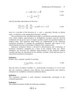
Figure 2.9. Expected values of probabilistically averaged Young modulus in matrix
0.21
0.212
0.214
0.216
0.218
0.22
0.222
4.00E-03 6.00E-03 8.00E-03 1.00E-02 1.20E-02 1.40E-02 1.60E-02 1.80E-02 2.00E-02
4 "teeth"
10 "teeth"
20 "teeth"
40 "teeth"
Figure 2.10. Probabilistically averaged Poisson ratio in fibre
46 Computational Mechanics of Composite Materials

0
0.05
0.1
0.15
0.2
0.25
0.3
0.35
4.00E-03 6.00E-03 8.00E-03 1.00E-02 1.20E-02 1.40E-02 1.60E-02 1.80E-02 2.00E-02
4 "bubbles"
10 "bubbles"
20 "bubbles"
40 "bubbles"
Figure 2.11. Probabilistically averaged Poisson ratio in matrix
As is expected, the resulting expected values of the homogenised Young
modulus both in the matrix and the fibre regions, and similarly the Poisson ratio,
are linear functions of the contact zone widths. The variances of the averaged
Young modulus are second or higher order functions of this variable and this order
is directly dependent on the number of interface defects.
Comparing Figures 2.8 with 2.9 and 2.12 with 2.13 it can be seen that the
Young modulus in the matrix contact zone is, for the present problem, much more
sensitive to variation of its parameters than the same modulus in the fibre
interphase. Larger coefficient of variation of this modulus is obtained in the matrix
interface region rather than in the fibre contact zone. On the other hand, the
homogenised elastic properties are derived by averaging their values in both
regions. Thus, greater changes in these properties can be expected in the matrix
because of the larger volume of bubbles related to the fibre teeth.
Another interesting effect (cf. Figures 2.12 and 2.13) is the increase of
variances of the homogenised Young modulus in the matrix contact zone for
increasing width of this zone and the number of bubbles. The reverse effect occurs

for the fibre side of the interface and its teeth. This is due to the fact that bubbles
occupy more than half of a volume of the corresponding contact zone, and teeth
less than a half.
Elasticity problems 47
16.6
16.8
17
17.2
17.4
17.6
17.8
4.00E-03 6.00E-03 8.00E-03 1.00E-02 1.20E-02 1.40E-02 1.60E-02 1.80E-02 2.00E-02
4 "teeth"
10 "teeth"
20 "teeth"
40 "teeth"
Figure 2.12. Variances of probabilistically averaged Young modulus in fibre
0
0.2
0.4
0.6
0.8
1
1.2
1.4
1.6
4.00E-03 6.00E-03 8.00E-03 1.00E-02 1.20E-02 1.40E-02 1.60E-02 1.80E-02 2.00E-02
4 "bubbles"
10 "bubbles"
20 "bubbles"

40 "bubbles"
Figure 2.13. Variances of probabilistically averaged Young modulus in matrix
48 Computational Mechanics of Composite Materials
2.2 Elastostatics of Some Composites
Elastic properties and geometry of Ω so defined result in the random
displacement field );(
ω
xu
i
and random stress tensor );(
ωσ
x
ij
satisfying the
classical boundary value problem typical for the linear elastostatics problem. Let
us assume that there are the stress and displacement boundary conditions,
t
Ω
∂
and
u
Ω
∂
respectively, defined on Ω . Let
ijkl
C be a random function of
1
C class
defined on the entire Ω region. Let
ρ

denote the mass density of a material
contained in
Ω and
i
f
ρ
denote the vector of body forces per a unit volume. The
boundary differential equation system describing this equilibrium problem can be
written as follows
);();();(
ωεωωσ
xxCx
klijklij
=
(2.48)
()
⎟
⎟
⎠
⎞
⎜
⎜
⎝
⎛
+=
i
j
j
i
ij

x
xu
x
xu
x
∂
ω∂
∂
ω∂
ωε
);(
);(
;
2
1
(2.49)
0)();(
,
=+
ijij
fx
ωρωσ
(2.50)
[]
[]
);(
ˆ
);(
ωω
xuExuE

ii
= ;
u
x Ω∈
∂
(2.51)
()
0);( =
ω
xuVar
i
;
u
x Ω∈
∂
(2.52)
[
]
[]
);();(
ωωσ
xtEnxE
ijij
= ;
t
x Ω∈
∂
(2.53)
(
)

0);( =
jij
nxVar
ωσ
;
t
x Ω∈
∂
(2.54)
for a=1,2, ,n and i,j,k,l=1,2.
Generally, the equation system posed above is solved using the well
established numerical methods. However it should first be transformed to the
variational formulation. Such a formulation, based on the Hamilton principle, is
presented in the next section. To have the formulation better illustrated, an example
of the periodic superconducting coil structure is employed. The stochastic non
homogeneities simulate the technological innacuracies of placing the
superconducting cable in the RVE. Its periodicity cell in that case is subjected to
horizontal uniform tension on its vertical boundaries to analyse the influence of the
stochastic defects on the probabilistic moments of horizontal displacements. The
stochastic variations of these displacements with respect to the thickness of the
interphase constructed are verified numerically. Stochastic computational
experiments are performed using the ABAQUS system and the program POLSAP
specially adapted for this purpose.
Elasticity problems 49
2.2.1 Deterministic Computational Analysis
The main idea of the numerical experiments provided in this section is to
illustrate the horizontal displacements fields and the shear stresses obtained for the
deterministic problem of uniform extension of the periodicity cell quarter. Both
Young modulus and Poisson ratio are assumed here as deterministic functions; for
the purpose of the tests, the program ABAQUS [1] is used together with its

graphical postprocessor. The periodicity cell quarter has been discretised by 224
rectangular 4 node plane strain isoparametric finite elements according to Figure
2.14.
Figure 2.14. Discretisation of the fibre-reinforced composite cell quarter
The symmetry displacement boundary conditions are applied on the horizontal
edges of the quarter as well as on the left horizontal edge, while the uniform
extension is applied on the right vertical edge of the RVE. The standard deviations
of the composite component Young moduli are taken as )(
1
e
σ
= 4.2 GPa, )(
2
e
σ
=
0.4 GPa and the stochastic interface defect data are approximated by the following
values:
[]
nE =3,
()
[]
15.005.0 == nEn
σ
,
[]
RrE 02.0= ,
()
40.81.0 −== ERr
σ

.
Probabilistically averaged values of the interphase elastic characteristics are
obtained from these parameters as follows
[]
GPaeE
k
82.3= ,
()
GPaeVar
k
48.1= ,
324.0=
k
ν
with the interphase thickness equal to
01040.
k
=∆
. Four numerical
experiments have been carried out for these parameters taking the values collected
in Table 2.1.
Table 2.1. Young modulus values of the interphase for particular tests
Test number 1 2 3 4
k
e
2
e
[]
k
eE

[]
()
kk
eeE
σ
⋅− 3
[]
()
kk
eeE
σ
⋅+ 3
50 Computational Mechanics of Composite Materials
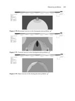
Horizontal displacement fields and the shear stress fields for particular
experiments are presented in Figure 2.15 and 2.19 (test no 1), Figure 2.16 and 2.20
for test no 2, Figure 2.17, 2.21 for test no 3 and Figure 2.18 for test no 4.
Comparing these results, it is seen that a decrease of the Young modulus value
lower than its expected value results in a jump of the horizontal displacements field
within and around the interphase. This effect can be interpreted as the possibility of
debonding of the composite components caused by the worsening of the interphase
elastic parameters, which confirms the usefulness of the presented mathematical
numerical model in the interphase phenomena analysis. It should be underlined that
in other models of interphase defects and contact effects at the interface, the
horizontal displacements have discontinuous character too. On the other hand,
increasing the Young modulus above its expected value does not introduce any
sensible differences in comparison with the traditional deterministic model for the
perfect interface.
Analysing the shear stresses fields
()
i

x
12
σ
collected in Figures 2.19 and 2.21 a
jump of the respective values of stresses at the boundary between the fibre and the
interphase region is observed in all cases. In the case of tests no. 1, 2 and 4 the
shear stress fields have quite similar characters differing one from another in the
interface regions placed near the horizontal and vertical edges of the periodicity
cell quarter. The
()
i
x
12
σ
field obtained for test no. 3 has decisively different
character: for almost the entire interface the jump of stresses between the matrix,
interphase and fibre regions is visible. It may confirm the previous thesis based on
the displacement results dealing with the usefulness of the model proposed for the
analysis of the interface phenomena.
+3.48E-35
+5.64E-05
+1.69E-04
+2.82E-04
+3.94E-04
+5.07E-04
+6.20E-04
+6.77E-04
+7.33E-04
Figure 2.15. Horizontal displacements for test no. 1
Elasticity problems 51

+3.49E-35
+5.64E-04
+1.69E-04
+2.82E-04
+3.95E-04
+5.08E-04
+6.21E-04
+6.77E-04
+7.34E-04
Figure 2.16. Horizontal displacements for test no. 2
+8.63E-35
+7.88E-05
+2.33E-04
+3.89E-04
+5.44E-04
+7.00E-04
+8.56E-04
+9.34E-04
+1.01E-03
Figure 2.17. Horizontal displacements for test no. 3
52 Computational Mechanics of Composite Materials
+3.28E-35
+5.85E-05
+1.67E-04
+2.79E-04
+3.91E-04
+5.02E-04
+6.14E-04
+6.70E-04
+7.26E-04

Figure 2.18. Horizontal displacements for test no. 4
-1.74E+02
+1.06E+02
+6.67E+02
+1.22E+03
+1.78E+03
+2.35E+03
+2.91E+03
+3.19E+03
+3.47E+03
Figure 2.19. The shear stresses for test no. 1
Elasticity problems 53
-1.45E+02
+1.37E+02
+7.02E+02
+1.26E+03
+1.83E+03
+2.39E+03
+2.96E+03
+3.24E+03
+3.52E+03
Figure 2.20. The shear stresses for test no. 2
-8.25E+01
+1.38E+02
+5.81E+02
+1.02E+03
+1.46E+03
+1.91E+03
+2.35E+03
+2.57E+03

+2.79E+03
Figure 2.21. The shear stresses for test no. 3
The general purpose of the computational experiments performed is to verify
the stochastic elastic behaviour of the composite materials with respect to
probabilistic moments of the input random variables: both the Young moduli of the
constituents as well as the stochastic interface defects parameters. The starting
point for such analyses is a verification of the probabilistically averaged Young
modulus in the interphase (example 1). This has been done by the use of the special
FORTRAN subroutine, while the next tests have been carried out using the 4 node
isoparametric rectangular plane strain element of the system POLSAP. Material
parameters of the composite constituents are taken in examples 1 to 3 as
54 Computational Mechanics of Composite Materials
=)(
1
eE 84.0 GPa,
1
ν
=0.22, 2.4)(
1
=e
σ
GPa, =)(
2
eE 4.0 GPa,
σ
() .e
2
04=
GPa,
2

ν
=0.34 (expected values and standard deviations of the Young modulus and
Poisson ratio, respectively).
2.2.2 Random Composite without Interface
Defects
The main aim of the numerical analysis is to verify numerically the elastic
behaviour of a fibre composite when the Young modulus of composite components
is Gaussian random variable. Moreover, numerical tests are carried out to state in
what way, for various contents of fibre (with round section) in a periodicity cell,
the random material properties of reinforcement and matrix influence the
displacement and stress distribution in the cell. A quarter of a fibre composite
periodicity cell is tested in numerical analysis and its discretisation is shown in
Figure 2.22.
Figure 2.22. Discretisation of the periodicity cell quarter
Numerical implementation enabling the computations is made using a 4 node
rectangular plane element of the program POLSAP (Plane Strain/Stress and
Membrane Element). The composite structure is subjected to the uniform tension
(100 kN/m) on a vertical cell boundary (60 finite elements with 176 degrees of
freedom). Vertical displacements are fixed on the remaining cell external
boundaries and the plane strain analysis is performed. Twelve numerical tests are
carried out assuming the fibre contents of 30, 40 and 50 % and the resulting
coefficients of variation are taken from Table 2.2.
Table 2.2. Coefficients of variation for different numerical tests
Test number
)(
1
e
α
)(
2

e
α
1 0.10 0.10
2 0.10 0.05
3 0.05 0.10
4 0.05 0.05
Elasticity problems 55
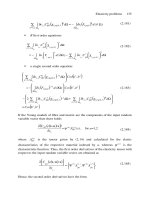
Each time the first two probabilistic moments of the displacements are
observed at the interface and on the tensioned vertical edge. In the case of stress
expectations, location and maximum value of reduced stress are examined. Figures
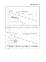
2.23 and 2.24 demonstrate radial displacement coefficients of variation of points
belonging to the fibre matrix boundary, which depend on the angle
β
describing
their locations on this boundary.
The results of test no. 1 (Table 2.2) are presented in Figure 2.23, and the next
figure shows the results of test no. 3; results of the remaining tests (no. 2 and 4)
agree with them respectively. In both cases coefficients of variation for
90=
θ
are omitted on the graphs because of their large values. For fibre contents equal to
50%, they are approximately 1.5 times greater than for
0=
θ
(disproportion of
the data would give an illegible picture). Therefore, it can be concluded that the
randomness of displacements on the considered boundary depends mainly on the
random character of fibre elastic properties, which means
2,11
];[)]([ Ω∈≅

∂αα
xexu
(2.55)
0.087
0.089
0.091
0.093
0.095
0.097
0.099
0.101
0.103
0 11.25 22.5 33.75 45 56.25 67.5 78.75
β
α
30% fiber contents
40% fiber contents
50% fiber contents
Figure 2.23. Coefficients of variation in test no. 1
56 Computational Mechanics of Composite Materials
0.044
0.045
0.046
0.047
0.048
0.049
0.05
0.051
0.052
0 11.25 22.5 33.75 45 56.25 67.5 78.75

β
α
30% fiber contents
40% fiber contents
50% fiber contents
Figure 2.24. Coefficients of variation in test no. 3
Fibre contents in periodicity cell influence also displacement coefficients of
variation on
12
Ω
∂
. This influence is visible especially at 450 ≤≤
θ
. For 40%
contents this decrease is not so sharp, and for 50% plane fraction the tendency is
the opposite: the coefficient increases up to about 1.5 times of the value obtained at
0=
θ
. In a physical way it may be interpreted as increasing the random measure
of uncertainty about displacements perpendicular to the fibre boundary of the
points belonging to its upper part with increasing fibre radius.
Figures 2.25 2.26 show displacement coefficients of the variation of horizontal
points belonging to a vertical, uniformly tensioned edge of periodicity cell obtained
in tests no. 1, 2, 3 and 4 respectively. Real numbers in decreasing order denote
height on the vertical tensioned edge on the horizontal axes of these figures.
Elasticity problems 57
0.078
0.08
0.082
0.084

0.086
0.088
0.09
0.092
0.094
0.096
0.098
0.5 0.42 0.33 0.25 0.17 0.08 0
α
30% fiber contents
40% fiber contents
50% fiber contents
Figure 2.25. Coefficients of variation in test no. 1
0.04
0.041
0.042
0.043
0.044
0.045
0.046
0.047
0.048
0.049
0.05
0.5 0.42 0.33 0.25 0.17 0.08 0
α
30% fiber contents
40% fiber contents
50% fiber contents
Figure 2.26. Coefficients of variation in test no. 2

58 Computational Mechanics of Composite Materials
0.08
0.082
0.084
0.086
0.088
0.09
0.092
0.094
0.096
0.098
0.5 0.42 0.33 0.25 0.17 0.08 0
α
30% fiber contents
40% fiber contents
50% fiber contents
Figure 2.27. Coefficients of variation in test no. 3
0.04
0.041
0.042
0.043
0.044
0.045
0.046
0.047
0.048
0.049
0.05
0.5 0.42 0.33 0.25 0.17 0.08 0
α

30% fiber contents
40% fiber contents
50% fiber contents
Figure 2.28. Coefficients of variation in test no. 4
The main conclusion from these results is that the random character of the
matrix elastic properties influences the randomness of displacements at the
tensioned edge of the composite specimen tested. Analogously to the previous
observations it can be written that
Elasticity problems 59
][)]([
2
exu
αα
≅ ;
σ
∂
ˆ
Ω∈x
(2.56)
Let us note that the random character of fibre stiffness has rather secondary
influence here. The curves describing displacement variation coefficients on the
edge are becoming less and less sharp together with an increase of the coefficients
of variation of the fibre Young modulus. Increase of fibre contents in the
periodicity cell, as expected, in all cases decreases variation coefficients of
tensioned edge displacements, which physically can be interpreted as increasing
stiffening of periodicity cell by the fibre.
Now, let us analyse expected values of maximum stresses (in MPa) in fibre and
matrix specified in Figure 2.29. Darker bars show the maximal stresses in the
matrix region, while lighter bars denote the fibre region, respectively.
Generally, it can be observed that the difference between the obtained expected

values and the results of deterministic tests is approximately equal to the
computational error. This difference would undoubtedly be much bigger if the
formula describing these values included a component connected with elasticity
tensor derivatives. The present version of computer program includes only the first
two components, which correspond with expected values of displacement
functions.
1 1.05 1.1 1.15 1.2 1.25 1.3 1.35 1.4 1.45
30(0)
30(2)
30(4)
40(0)
40(2)
40(4)
50(0)
50(2)
50(4)
Figure 2.29. Expected values of maximal stresses
The results obtained lead to the conclusion that the most important factor
influencing the value of maximum stresses is unquestionably the fibre radius, cf.
60 Computational Mechanics of Composite Materials
Figure 2.29. In the case of the matrix region, maximum stresses increase
approximately in direct proportion to fibre radius increment
RxE ≈)]([
max
σ
;
2
Ω∈x
(2.57)
To get an analogous relation for maximum stress appearing in the fibre, it is

necessary to make a more precise numerical analysis. In tested examples with
plane fractions of 30, 40 and 50% extremum appeared at 40% contents of fibre in
the periodicity cell. Another factor, which influences the expected values of
maximum stresses within a given material, is its coefficient of variation for the
Young modulus. The following relation can be formulated:
][)]([
max i
exE
ασ
≈ ;
i
x Ω∈
(2.58)
Finally, it can be observed that there is a third order influence of stronger
material random changes of elastic features on maximum stresses in the matrix,
especially with decreasing fibre contents in the RVE.
In the context of the present numerical analysis of maximum stresses it should
be added that, apart from changes in the expected values of these stresses, a change
of their locations was observed. In order to state the relation between the location
of changes in the direction of the stress functions extremum and fibre radius
increment it would be necessary to consider a wider range of this radius variation
(equivalent to, for example, a surface fraction of 10 to 60%) with simultaneously
increasing the number of tests (each 1 to 5% for example). The most essential thing
would be, however, creating a mesh much more precise than the one used in the
above tests, especially near the composite interface, where we have, of interest to
us, maximum stresses.
2.2.3 Fibre reinforced Composite with Stochastic
Interface Defects
The subject of the third numerical example is the fibre reinforced periodic
composite, which has been discretised in Figure 2.30 as a cell quarter with smaller

contact zones on the left and with larger ones on the right. The composite structure
is subjected to uniform tension on the vertical cell boundary. Six numerical tests
have been performed assuming interphases with different values of the total
number of defects (in turn: 0%, 25% and 50% of the interface length). In each test,
the first two probabilistic moments of the displacements are observed on the phase
boundary and on the vertical edge subjected to tension and the coefficient of
variation for displacements.
Elasticity problems 61
Figure 2.30. Quarter periodicity cell mesh for the SFEM analysis
0.0009
0.0014
0.0024
0.0034
0.0044
0 11.3 22.5 33.8 45 56.3 67.5 78.8
0%
bubbles
25%
bubbles
50%
bubbles
β
E[u
h
]
Figure 2.31. Expected values of horizontal displacement at the interface
0.049
0.0494
0.0498
0.0502

0.0506
0 11.3 22.5 33.8 45 56.3 67.5 78.8
0%
bubbles
25%
bubbles
50%
bubbles
β
α(u
h
)
Figure 2.32. Coefficients of variation of horizontal displacements at the interface
62 Computational Mechanics of Composite Materials
E[u
h
]
2.00E-02
3.00E-02
4.00E-02
5.00E-02
6.00E-02
0 0.08 0.17 0.25 0.33 0.42 0.5
0% bubbles
25% bubbles
50% bubbles
h
Figure 2.33. Expected values of horizontal displacements at the tensioned edge
α(u
h

)
0.08
0.084
0.088
0.092
0.096
0.10
0 0.08 0.17 0.25 0.33 0.42 0.50
0% bubbles
25% bubbles
50% bubbles
h
Figure 2.34. Coefficients of variation of horizontal displacements at the tensioned edge
The expected values of the displacements and their coefficients of variation are
placed on the vertical axes of all figures. The angle β, which determines the
location of a point on the fibre matrix interface with respect to the x or y
coordinate on the tensioned edge, and which is marked on the vertical axes.
A further general observation is a direct proportionality between the number of
interface defects and the volume of the contact zone as well as the expected values
or coefficients of variation of these displacements. Small differences occur in the
interface expected values of displacements for larger values of the angle β.
By comparing the coefficients of variation of the interface displacements
(Figure 2.32 and 2.34) quite different forms for the relation between these
coefficients and the angle β are observed. The model with a large contact zone
shows a high sensitivity to the number of defects and the changes for the small
contact zone are proportional. In the case of the coefficients of variation of the
tensioned edge horizontal displacement both the models give approximately
reversed effects. For example a small contact zone causes larger coefficients for
smaller β values than for the larger ones (Figure 2.32). For both sizes of the contact
Elasticity problems 63

zones the changes in the coefficient α are inversely proportional to the increase in
the number of discontinuities and show some similarity.
Finally, in both models the expected values of the displacement are quite
similar with respect to their locations. In the large contact zone (Figure 2.31 and
2.33) the differences between the obtained expected values of displacements for
0%, 25% and 50% of discontinuities are more significant.
2.2.4 Stochastic Interface Defects in Laminated
Composite
The two component layered composite has been tested in this example. The
discretisation into 72 finite elements and 233 degrees of freedom as well as the
mixed boundary conditions is shown in Figure 2.35. Both layers have been
uniformly extended in the opposite directions to verify the influence of interphase
between them on the overall behaviour of the structure.
Figure 2.35. Two layer laminate in the computational shear test
Ten numerical experiments have been carried out in the example: the
deterministic problem (test d) and the stochastic one without interface defects
(test s). In the next experiments the standard deviations of the defects are taken as
][1.0][ rEr ⋅=
σ
, ][1.0][ nEn ⋅=
σ
, and the expected values are shown in Table 2.3
(contribution of the boundary occupied by bubbles to the total boundary is given in
brackets).
Table 2.3. The expected values of the interface defects tested
Test 1 Test 2 Test 3 Test 4 Test 5 Test 6 Test 7 Test 8
E
[
r
] 5.0E-2 5.0E-2 5.0E-2 5.0E-2 1.0E-1 1.0E-1 1.0E-1 1.0E-1

E
[
n
] 5
(10%)
10
(20%)
15
(30%)
20
(40%)
5
(20%)
10
(40%)
15
(60%)
20
(80%)
The results of the analyses have been collected in Table 2.3, which shows the
expected values and the coefficients of variation of the displacements and are
64 Computational Mechanics of Composite Materials
generally consistent with those obtained experimentally (in the range of expected
values). The increases of the expected values in comparison to the results obtained
in test d and test s are included also in this table. The coefficients of variation of
the horizontal displacements for smaller and greater interphase are presented in
Figure 2.36 and 2.37 as a function of the location of a point on the
2
Ω boundary.
On the horizontal axis the height of the point (h) in decreasing order is presented:

the coordinate 2.5 denotes the point belonging to the interface and
1
Ω region on the
extended
2
Ω boundary, while the coordinate 5.0 denotes the point belonging to the
upper
2
Ω boundary.
Table 2.4. The expected values and coefficients of variation of the displacements tested
Test-d test-s test 1 test 2 test 3 test 4 test 5 test 6 test 7 Test
8
E[q]
(E-2)
1.924
2.610
1.939
2.633
2.049 2.089 2.134 2.188 2.686 2.844 3.065 3.408
∆E[q]
(%)
-0.8
-0.9
0.0
0.0
5.7 7.7 10.1 12.8 2.0 8.0 16.4 29.4
α[q]
- 0.082 0.078 0.080 0.083 0.089 0.088 0.098 0.120 0.158
Generally, all the results computed show that the most sensitive region to the
input random parameters is the point located on the weaker material (matrix) and

the interphase on the extended
2
Ω boundary. Moreover, analysing the increases of
the expected values of horizontal displacements on the tensioned boundary the
significant influence of the stochastic interface defects introduced can be observed.
In all tests performed the displacements obtained are greater than for the
composites without defects between the composite constituents.
Moreover, the increases of the displacements analysed increase faster than the
increases of the total length of the boundary occupied by the bubbles, which
follows the stochastic nonlinearity of the model presented. The diagrams of the
displacements have analogous characteristics to those obtained for the coefficients
of variation presented later. However, considering the large disproportions between
the values computed near the interphase and outside it, these graphs have been
omitted.
Elasticity problems 65
0.044
0.054
0.064
0.074
0.084
0.094
0.104
5 4.38 3.75 3.13 2.57 2.5
test-s
test1
test2
test3
test4
h
α(u

h
)
Figure 2.36. Coefficients of variation of horizontal displacements for shear test (I)
0.045
0.065
0.085
0.105
0.125
0.145
0.165
5 4.38 3.75 3.13 2.63 2.5
test-s
test 5
test 6
test 7
test 8
α
(u
h
)

h
Figure 2.37. Coefficients of variation of horizontal displacements for shear test (II)
Comparing the coefficients of variation of the horizontal displacements it is
seen that, especially in case of tests no. 5 to 8 (the interphase twice as large as for
tests 1 to 4) the significant increase of these displacements is about 95% in case of
test no. 8. These increases are analogous to the increases of expected values greater
for displacements rather than the corresponding increases of total length of
interface boundary occupied by the bubbles.
As can be expected, the statistical response of the laminate should depend on

the contrast between stronger and weaker layer material properties, interphase
elastic parameters, the total number of layers in the composite etc. Essentially
different situation can be observed when both material properties and external load
are introduced as random variables [273].
66 Computational Mechanics of Composite Materials
2.2.5 Superconducting Coil Cable Probabilistic
Analysis
The main ideas of the experiment [193] are as follows: (i) comparison of the
stochastic behaviour of the superconducting coil cable in the original geometry
with the model in which the technological nonhomogeneities have been
probabilistically averaged; (ii) verification of the model sensitivity to the assumed
thickness of the interphase introduced.
The example of the RVE analysed is presented in Figures 2.38 and 2.39 (all
geometric dimensions are given in mm). A single discontinuity is modelled by
complementing two circle quarters (teeths with their sharp sides directed to the
interior of the superconducting cable). Their radii are equal to 1.5 mm for defects
on the interface superconducting cable tube and 2.0 mm for defects on the
interface cable jacket. The periodicity cell is subjected to a horizontal uniform
tension on its vertical boundaries; due to symmetry only one quarter of this cell is
employed. Displacement boundary conditions on all the remaining external
boundaries are assumed to satisfy the symmetry conditions.
Figure 2.38. Superconducting coil cable RVE geometry
Figure 2.39. Quarter periodicity cell mesh for the superconductor
Elasticity problems 67
The elastic properties and their probabilistic characteristics of the RVE
components, the expected values and the standard deviations of Young moduli,
Poisson ratios and Kirchhoff moduli are collected in Table 2.5.
Table 2.5. Elastic characteristics of composite components
Material
E

[
e
] [GPa] σ(
e
) [GPa]
ν
G
[GPa]
Tube 205.0 8.0 0.265 81.0
Superconductor 182.0 0.0 0.300 70.0
Jacket 126.0 12.0 0.311 48.0
Insulation 36.0 0.0 0.210 11.0
The following tests are performed: deterministic test including defects non
averaged (test 1), an experiment without defects (test 2), an experiment with
defects averaged in the interphase (test 3) or over the finite elements which they
belong to (test 4). The first two probabilistic moments of the displacements are
observed in each test on the interface determined by a radius equal to 9.0 mm
(between the lower superconductor interphase and the superconductor region).
Four additional tests are performed in test 3 to verify the results variations with
respect to the interphase thicknesses: test 3A, where the thickness is equal to the
expected value of the relevant geometric dimensions of interface defects, test 3D
with thickness given by eqn (2.22) and tests 3B and 3C with the intermediate
thicknesses.
The results of these computations due to tests numbered 1 to 4 are presented in
Figures 2.40 and 2.41: the expected values of the horizontal displacements and
their coefficients of variation. The first two moments are marked on the vertical
axes of these figures, while the angle β, which determines the location of a point
on the interface considered with respect to the x coordinate on the horizontal axes.
The results of tests 3A to 3D are collected in Table 2.6 presented below the figures.
The expected values of displacements observed (in mm) are given in the upper row

of each table cell and the coefficients of variation in the lower one.
0.6
0.7
0.8
0.9
1
1.1
0 9 18 27 36 45
test 1
test 2
test 3
test 4
Figure 2.40. Expected values of horizontal displacements at the tensioned edge
68 Computational Mechanics of Composite Materials
0.019
0.021
0.023
0.025
0.027
0.029
0.031
0.033
0.035
0 9 18 27 36 45
test 2
test 3
test 4
Figure 2.41. Coefficients of variation of horizontal displacements at the tensioned edge
Table 2.6. The expected values and the coefficients of variation of horizontal displacements
β [°] Test 3A Test 3B Test 3C Test 3D

0 1.066
0.0241
1.069
0.0237
1.078
0.0235
1.085
0.0233
9 1.047
0.0239
1.053
0.0238
1.057
0.0234
1.062
0.0232
18 0.985
0.0236
0.993
0.0234
0.994
0.0231
1.003
0.0230
27 0.895
0.0239
0.897
0.0235
0.908
0.0234

0.910
0.0231
36 0.783
0.0241
0.784
0.0238
0.784
0.0235
0.790
0.0232
45 0.631
0.0212
0.634
0.0212
0.639
0.0213
0.645
0.0214
Generally, it can be observed that in all stochastic tests the expected values of
horizontal displacements are greater than the corresponding values obtained from
deterministic tests, which follow equation (1.134). The greatest expected values of
displacements observed are obtained for test 4: from 50% (for β≈0°) to 100% (for
β≈80°) greater than in the remaining tests. Analogous observation can be done for
the coefficients of variation. Generally, these facts follow the great variances of the
Young moduli in finite elements containing defects averaged in comparison to the
remaining elements.
On the basis of these results it can be stated that the observed probabilistic
moments of displacements are strongly sensitive to the scale of the composite
structure, which probabilistic averaging is applied in. A rapid decrease of the total
area of the region averaged results in a significant increase of the effective Young

modulus and much smaller increases of the expected values for the displacements.
Further, the expected values obtained in test 2 (without including interface defects
in any form) give the most exact results of the horizontal displacements computed
Elasticity problems 69
in the deterministic model. However, for β≈30°, which corresponds to the defects
location, the best approximation is obtained in test 3 (with interphase zones
introduced).
Finally, let us consider the stochastic variations of the interface horizontal
displacements to the interphase zone thicknesses illustrated by the results collected
in Table 2.6. It can be observed that increasing thickness causes a small increase of
the horizontal displacements and a decrease of the coefficients of variation. The
decrease (or increase) has a linear character and the maximum increment is no
greater than 2% of the values considered. It confirms the possibility of using the
model presented in the numerical analysis of stochastic non homogeneities
(especially interface defects) in composite materials. To verify the applicability of
the model presented this sensitivity should be discussed as a function of interface
defects and elastic properties of composite component stochastic parameters.
Let us note that the SFEM methodology can be applied in further analyses for
numerical modelling of random both uncoupled and coupled thermal, electric or
magnetic fields in various superconducting structures [221,385]. A common
application of the stochastic perturbation technique with computational plasticity
algorithms will enable us to perform modelling of interface debonding in the case
of laminates and fibre-reinforced composites, which will essentially extend our
knowledge of composites behaviour in relation to the existing models
[251,384,386].