Computational Mechanics of Composite Materials part 13 potx

Multiresolutional Analysis 345
7.5 Free Vibrations Analysis
The main idea of homogenisation problem solution now is a separate
calculation of the effective elastic modulus and spatial averaging of the mass
density, where the first part only needs multiresolutional approach [189]. The
alternative wavelet based methodology is presented in [328,329], for a plate wave
propagation in [152], whereas some classical unidirectional examples are contained
in [330]. Let us consider the following differential equilibrium equation:
)()()()( xMxu
dx
d
xIxe
dx
d
=
⎟
⎠
⎞
⎜
⎝
⎛
− ; ]1,0[∈x
(7.79)
where e(x), defining material properties of the heterogeneous medium, varies
arbitrarily on many scales together with the inertia momentum I(x). A
multiresolutional homogenisation starts now from the following decomposition of
the equilibrium equation:
⎪
⎪
⎩
⎪

⎪
⎨
⎧
=
−=
)()(
)(
)(
)()(
xIxe
xv
xu
dx
d
xMxv
dx
d
(7.80)
to determine the homogenised coefficient e
(eff)
constant over the interval ]1,0[∈x ,
which takes the integral form
∫
⎟
⎟
⎠
⎞
⎜
⎜
⎝

⎛
⎟
⎟
⎠
⎞
⎜
⎜
⎝
⎛
−
+
⎟
⎟
⎠
⎞
⎜
⎜
⎝
⎛
⎟
⎟
⎠
⎞
⎜
⎜
⎝
⎛
=
⎟
⎟

⎠
⎞
⎜
⎜
⎝
⎛
−
⎟
⎟
⎠
⎞
⎜
⎜
⎝
⎛
−−
x
dt
tMtv
tu
tIte
v
u
xv
xu
0
11
)(
0
)(

)(
00
)()(0
)0(
)0(
)(
)(
(7.81)
On the other hand, the reduction algorithm between multiple scales of the
composite consists in determination of such effective tensors
)eff(
B ,
)eff(
A ,
)eff(
p
and
)eff(
q , such that
()
∫
⎟
⎟
⎠
⎞
⎜
⎜
⎝
⎛
+

⎟
⎟
⎠
⎞
⎜
⎜
⎝
⎛
=++
⎟
⎟
⎠
⎞
⎜
⎜
⎝
⎛
+
x
effeffeffeff
dtp
tv
tu
Aq
xv
xu
BI
0
)()()()(
)(

)(
)(
)(
λ
(7.82)
It can be shown that
⎟
⎟
⎠
⎞
⎜
⎜
⎝
⎛
−
=
⎟
⎟
⎠
⎞
⎜
⎜
⎝
⎛
=
00
20
;
00
00

21
)()(
CC
AB
effeff
(7.83)
where
346 Computational Mechanics of Composite Materials
()
∫∫
−
==
1
0
2
1
2
1
0
1
)()(
;
)()( tIte
dtt
C
tIte
dt
C
(7.84)
Furthermore, for f(x)=0 there holds 0

)()(
==
effeff
qp , while, in a general case,
)(eff
B
and
)(eff
A
do not depend on p and q. Finally, the homogenised ODEs are
obtained as
()
⎪
⎩
⎪
⎨
⎧
−=
=
)(2)(
)(
21
)(
xvCCxu
dx
d
fxv
dx
d
eff

(7.85)
which is essentially different to the classical result of the asymptotic
homogenisation shown previously. Effective mass density of a composite can be
derived by a spatial averaging method, which is completely independent from the
space configuration and periodicity conditions of a composite structure. The
relation is used for classical and wavelet based homogenisation approaches as
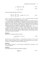
well. Finally, the following variational equation is proposed to achieve the
dynamic equilibrium for the linear elastic system [208]:
()
∫∫∫∫
Ω∂ΩΩΩ
Ω∂+Ω=Ω+Ω
σ
δδρδεεδρ
dutdufdCduu
iiiiklijijklii
(7.86)
where
i
u
mass density defined by the elasticity tensor )(xC
ijkl
x); the
vector
i
t denotes the stress boundary conditions defined on Ω∂⊂Ω∂
σ
.
An analogous equation rewritten for the homogenised heterogeneous medium
has the following form:

()
∫∫∫∫
Ω∂ΩΩΩ
Ω∂+Ω=Ω+Ω
σ
δδρδεεδρ
dutdufdCduu
iiii
eff
klij
eff
ijklii
eff
)()()(
(7.87)
where all material properties of the real system are replaced with the effective
parameters. Let us introduce a discrete representation of the function
i
u by the
following vector of the generalised coordinates for the needs of the Finite Element
Method implementation:
() () ()
αααα
φφ
qxqxxu
E
e
e
iii
⎥

⎦
⎤
⎢
⎣
⎡
==
∑
=1
)(
(7.88)
Multiresolutional Analysis 347
which gives us for the strain tensor components
() () ()
[]
()
ααααα
φφε
qxBqxxx
ijijjiij
=+=
,,
2
1
(7.89)
The matrix description for stiffness, mass, damping components as well as the
RHS vector is proposed as
Ω=
∫
Ω
dBBCK

klijijkl
βααβ
, Ω=
∫
Ω
dBBCK
klij
eff
ijkl
eff
ijkl
βα
)()(
(7.90)
Ω=
∫
Ω
dM
ii
βααβ
φφρ
, Ω=
∫
Ω
dM
ii
effeff
βααβ
φφρ
)()(

(7.91)
()
Ω∂+Ω=
∫∫
Ω∂Ω
dtdfQ
iiii
σ
ααα
φφρ
()
Ω∂+Ω=
∫∫
Ω∂Ω
dtdfQ
iiii
effeff
σ
ααα
φφρ
)()(
(7.92)
Usually, it is assumed that the damping matrix can be decomposed into the part
having the nature of body forces with the proportionality coefficient c
M
and the rest
composes the viscous stresses multiplied by the quantity c
K
, so that
αβαβαβ

KcMcC
KM
+= ,
)()()( eff
K
eff
M
eff
KcMcC
αβαβαβ
+=
(7.93)
After such a discretisation of all the state functions and structural parameters in
(7.86) and (7.87), the following matrix equation for real heterogeneous system is
obtained:
αβαββαββαβ
QqKqCqM =++
(7.94)
Therefore, the equivalent homogenised dynamic equilibrium equation to be
solved for the deterministic problem has the form
)()()()( effeffeffeff
QqKqCqM
αβαββαββαβ
=++
(7.95)
where the barred unknowns represent the response of the homogenised system. The
RHS vector is equal to 0, so the homogenised operators are to be computed for the
LHS components only in the case of free vibrations. The eigenvalues and
eigenvectors for the undamped systems are determined from the following matrix
equations:

(
)
0
)(
=Φ−
βγαβααβ
ω
MK ;
(
)
0
)(
)(
)(
=Φ−
βγ
αβ
α
αβ
ω
effeff
MK
(7.96)
348 Computational Mechanics of Composite Materials
which are implemented and applied below to compare homogenised and real
composites.
Numerical analysis illustrating presented ideas is carried out in two separate
steps. First, homogenised characteristics of a periodic composite determined thanks
to different homogenisation models are obtained by the use of the MAPLE
symbolic computation. Then, the FEM analysis of the free vibration problems is

made for the simply supported two , three and five bay periodic beams, made of
the original and homogenised composites, having applications in aerospace and
other engineering structures subjected to vibrations [189]. The periodicity is
observed in macroscale (equal length of each bay) as well as in microstructure –
each bay is obtained by reproduction of the identical RVE whose elastic modulus
is defined by some wavelet function.
The formulae presented above are implemented in the program MAPLE
together with the spatial averaging method in order to compare the homogenised
modulus computed by various ways (spatial averaging, classical and
multiresolutional) for the same composite. Figure 7.22 illustrates the variability of
this modulus along the RVE, where the function e(x) is subtracted from the
following Haar and Mexican hat wavelets:
⎩
⎨
⎧
≤<
≤≤
=
15.090.2
5.00;90.20
)(
xE
xE
xh
(7.97)
⎟
⎟
⎠
⎞
⎜

⎜
⎝
⎛
−
−
+=
2
2
2
2
3
2
exp
1
2
1
2)(
σσ
σπ
xx
xm
-0.4
(7.98)
as
)x(mE.)x(h.)x(e 902010 +=
(7.99)
Mass density of the composite is adopted as the wavelet of similar nature
⎩
⎨
⎧

≤<
≤≤
=
15.0;20
5.00;200
)(
~
x
x
xh
(7.100)
with
)x(m.)x(h
~
.)x( 5050 +=ρ
(7.101)
which is displayed in Figure 7.23.
Multiresolutional Analysis 349
Figure 7.22. Wavelet-based definition of elastic modulus in the RVE
Figure 7.23. Wavelet-based definition of mass density in the RVE
The final form of these functions is established on the basis of the mathematical
conditions for homogenisability analysed before as well as to obtain the final
variability of composite properties similar to the traditional multi-component
structures. Let us note that classical definition of periodic composite material
properties contained the piecewise constant Haar basis only.
The following homogenised material properties are obtained from this input:
137.56
)(
=
eff

ρ
,9548114 E.e
)av(
= > 921760 E.e
)wav,eff(
= > 943735 E.e
)eff(
= ,
which means that for this particular example, the highest value is obtained for the
spatial averaging method, then – for the wavelet approach at least – for classical
homogenisation method based on the small parameter assumption. The
effectiveness of such homogenisation results is verified in the next section by
comparison of the eigenvalues and the eigenfunctions of some periodic composite
beams being homogenised with its real material distribution.
The free vibration problems for two , three and five bay periodic beams are
solved using the classical and homogenisation based Finite Element Method
implementation [13,387]. The unitary inertia momentum is taken in all
computational cases, ten periodicity cells compose each bay, while material
properties inserted in the numerical model are calculated from (a) spatial
averaging, (b) the classical homogenisation method and (c) the multiresolutional
350 Computational Mechanics of Composite Materials
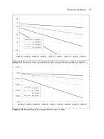
scheme proposed above and compared against the real structure response. The
results of eigenproblem solutions are presented as the first 10 eigenvalue variations
for the beams in Figures 7.24, 7.26 and 7.28 together with the maximum
deflections of these beams in Figures 7.25, 7.27 and 7.29 – the resulting values are
marked on the vertical axes, while the number of the eigenvalue being computed is
on the horizontal axes. The particular solutions for 1
st
, 2
nd

, 3
rd
and lower next
eigenvalues are connected with the continuous lines to better illustrate
interrelations between the results obtained in various homogenisation approaches
related to the real composite model.
ω
α
α
Figure 7.24. Eigenvalues progress for various two bay composite structures
α
α
Figure 7.25. Maximum deflections for the eigenproblems of two bay composite structures
Multiresolutional Analysis 351
ω
α
α
Figure 7.26. Eigenvalues progress for various three bay composite structures
α
α
Figure 7.27. Maximum deflections for the eigenproblems of three bay composite structures
352 Computational Mechanics of Composite Materials
ω
α
α
Figure 7.28. Eigenvalues progress for various five bay composite structures
α
α
Figure 7.29. Maximum deflections for the eigenproblems of five bay composite structures
As can be observed, the eigenvalues obtained for various homogenisation

models approximate the values computed for the real composite with different
accuracies, and the maximum deflections are the same. The weakest efficiency in
eigenvalue modelling is detected in the case of a spatially averaged composite –
the difference in relation to the real structure results increases together with the
eigenvalue number. Wavelet based and classical homogenisation methods give
more accurate results – the first method is better for smaller numbers of bays (and
the RVEs along the beam) see Figure 7.24, whereas the classical homogenisation
approach is recommended in the case of increasing number of the bays and the
RVEs, cf. Figures 7.26 and 7.28. The justification of this observation comes from
the fact that the wavelet function appears to be of less importance for the
Multiresolutional Analysis 353
increasing number of periodicity cells in the structure. Another interesting result is
that the efficiency of the approximation of the maximum deflections for a multibay
periodic composite beam by the deflections encountered for homogenised systems
increases together with an increase of the total number of bays. The agreement
between the eigenvalues for the real and homogenised systems will allow usage of
the stochastic spectral finite element techniques [261], where the random process
expansions are based on the relevant eigenvalues.
Finally, let us note that further extensions of this model on vibration analysis of
fibre-reinforced composites [60] using 2D wavelets are possible. An application of
wavelet technique is justified by the fact that the spatial distribution of the
constituents in the composite specimen is recently a subject of digital image
analysis [341]. On the other hand, chaotic behaviour of real and homogenised
composites [199] may be studied in the above context.
7.6 Multiscale Heat Transfer Analysis
The idea of transient heat transfer homogenisation, i.e. calculation of the
effective material parameters, consists in separate spatial averaging of the
volumetric heat capacity and the solution (analytical or numerical) of the heat
conduction homogenisation problem [15,165,166,195]. As is illustrated below, the
final form of the effective heat conductivity coefficient varies with the composite

model, whereas a composite with piecewise constant properties and/or defined by
some wavelet functions can have the same homogenised volumetric heat capacity.
That is why first the heat conduction equation for a 1D periodic composite is
homogenised and the effective heat capacity and mass density are determined by a
spatial averaging approach. The multiresolutional homogenisation method starts
from the following decomposition of heat conduction equation [23,55] as follows:
⎪
⎪
⎩
⎪
⎪
⎨
⎧
=
−=
)(
)(
)(
)()(
xk
xv
xT
dx
d
xQxv
dx
d
(7.102)
The main goal is to determine the homogenised coefficient k
(eff)

being constant over
the interval
]1,0[∈x
. Therefore, the equation system (7.102) can be rewritten as
∫
⎟
⎟
⎠
⎞
⎜
⎜
⎝
⎛
⎟
⎟
⎠
⎞
⎜
⎜
⎝
⎛
−
+
⎟
⎟
⎠
⎞
⎜
⎜
⎝

⎛
⎟
⎟
⎠
⎞
⎜
⎜
⎝
⎛
=
⎟
⎟
⎠
⎞
⎜
⎜
⎝
⎛
−
⎟
⎟
⎠
⎞
⎜
⎜
⎝
⎛
−
x
dt

tQtv
tT
tk
v
T
xv
xT
0
1
)(
0
)(
)(
00
)(0
)0(
)0(
)(
)(
(7.103)
354 Computational Mechanics of Composite Materials
On the other hand, the reduction algorithm between multiple scales of the
composite consists in the determination of such effective operators
)eff(
B ,
)eff(
A ,
)eff(
p ,
)eff(

q , that
()
∫
⎟
⎟
⎠
⎞
⎜
⎜
⎝
⎛
+
⎟
⎟
⎠
⎞
⎜
⎜
⎝
⎛
=++
⎟
⎟
⎠
⎞
⎜
⎜
⎝
⎛
+

x
effeffeffeff
dtp
tv
tT
Aq
xv
xT
BI
0
)()()()(
)(
)(
)(
)(
λ
(7.104)
It can be shown that
⎟
⎟
⎠
⎞
⎜
⎜
⎝
⎛
−
=
⎟
⎟

⎠
⎞
⎜
⎜
⎝
⎛
=
00
20
;
00
00
21
)()(
kk
AB
effeff
(7.105)
where
(
)
∫∫
−
==
1
0
2
1
2
1

0
1
)(
;
)( tk
dtt
k
tk
dt
k
(7.106)
Furthermore, for Q(x)=0 there holds 0==
)eff()eff(
qp (in a general case,
)eff(
B and
)eff(
A do not depend on p and q). Finally, the system of two
homogenised ordinary differential equations are obtained as
()
⎪
⎩
⎪
⎨
⎧
−=
=
)(2)(
)(
21

)(
xvkkxT
dx
d
qxv
dx
d
eff
(7.107)
which is essentially different than the classical result of the asymptotic
homogenisation shown previously. Let us observe that in the case of the heat
conductivity variability in two separate scales
⎟
⎠
⎞
⎜
⎝
⎛
=
ε
x
xkk , the multiresolutional
scheme reduces to the classical macro micro methodology where the following
limits are demonstrated:
11
0
)(lim kk =
→
ε
ε

and
0)(lim
2
0
=
→
ε
ε
k
(7.108)
Finally, the effective volumetric heat capacity of a composite is determined by
the spatial averaging method, which relation does not depend either on the space
configuration or on the periodicity conditions of a composite structure, and is used
for both classical and multiresolutional homogenisation approaches.
Multiresolutional Analysis 355
Using traditional FEM discretisation of the temperature field and its gradients
by the nodal temperatures vector
α
θ
[7,21,213,283]
() ()
αα
θ
yHyT = ; α=1, ,N
(7.109)
() ()
δδ
θ
yHyT
yy ,,

= ; δ=1, ,N
(7.110)
the following transient problems are solved:
averaged material properties
)()()( avavav
PKC
δβδββδβ
θθ
=
′
+
′
, N, ,,, 21=
β
δ ,
(7.111)
asymptotically homogenised material properties
)()()( effeffeff
PKC
δβδββδβ
θθ
=
′′
+
′′
, N, ,,, 21=
β
δ ,
(7.112)
for multiresolutionally homogenised material properties in the system

weffweffweff
PKC
)()()(
δβδββδβ
θθ
=
′′′
+
′′′
, N, ,,, 21=
β
δ .
(7.113)
Numerical analysis illustrating the ideas presented is carried out in two separate
steps. First, homogenised characteristics of a periodic composite obtained through
different homogenisation models are determined by the use of MAPLE symbolic
computations. This numerical approach is used also to verify input parameter
variability of the homogenised characteristics as well as design sensitivities of
these characteristics with respect to the contrast parameter (interrelation between
the heat conductivities of the composite components) and the interface location
along the RVE length (g). Next, the FEM analysis of transient heat transfer is made
to discuss the differences between temperature and heat flux histories resulting
from various homogenisation models contrasted with the real system. An
alternative way to model multiscale transient heat transfer phenomena in
composites is to expand the classical FEM methodology using a wavelet based
both space and time adaptive numerical methods, as it was discussed in [17], for
instance; the other aspects of this problem have been studied in [40].
The formulae for effective heat conductivity are implemented in the program
MAPLE together with the spatial averaging method in order to compare the
homogenised modulus computed by various ways for the same composite. Figure

7.30 illustrates the variability of this modulus along the RVE, where the function
k(x) is subtracted from the following Haar basis and Mexican hat wavelet:
⎩
⎨
⎧
≤<
≤≤
=
15.0;
5.00;
)(
2
1
xk
xk
xh
(7.114)
356 Computational Mechanics of Composite Materials
⎟
⎟
⎠
⎞
⎜
⎜
⎝
⎛
−
−
+=
2

2
2
2
3
2
exp
1
2
1
2)(
σσ
σπ
xx
xm
-0.5
(7.115)
as
)x(m.)x(h)x(k 0010+=
(7.116)
Further, volumetric heat capacity of the composite is adopted as the wavelet of
a similar form
⎩
⎨
⎧
≤<
≤≤
=
15.0;
5.00;
)(

~
22
11
xc
xc
xh
ρ
ρ
(7.117)
with
)x(m)x(h
~
)x(c)x(
3
10+=ρ
(7.118)
which is demonstrated in Figure 7.31.
Figure 7.30. Wavelet-based definition of heat conductivity coefficient in RVE
Multiresolutional Analysis 357
Figure 7.31. Wavelet-based definition of the volumetric heat capacity in RVE
The final form of these functions is established on the basis of the mathematical
conditions for homogenisability analysed before as well as to obtain the final
variability of composite properties similar to the traditional multi-component
structures. Let us note that the classical definition of periodic composite material
properties contained the piecewise constant Haar basis only.
Symbolic computations of the MAPLE system were used next to perform the
comparison between the spatial averaging, classical and multiresolutional
homogenisation scheme for various values of the composite constituents contrast
and the interface position g. The results of the analysis are demonstrated in Figures
7.32, 7.33 and 7.34, respectively. However it could be expected, the results of

spatial averaging are globally the greatest for the entire variability ranges of the
design parameters, while the interrelation between the classical and wavelet-based
methods differ on the input parameter values.
The separate, very interesting numerical problem would be to determine the
intersection of the surfaces plotted in Figures 7.33 and 7.34. It can be interpreted as
the curve equivalent to such pairs of the contrast and interface location in the RVE
for which both multiresolutional and classical homogenisation methods can result
in the same effective quantity. Let us note that the problem is independent from
physical interpretation of homogenised characteristics).
358 Computational Mechanics of Composite Materials
Figure 7.32. Parameter variability of k
(av)
Figure 7.33. Parameter variability of k
(eff)
Figure 7.34. Parameter variability of k
(eff)w
Multiresolutional Analysis 359
Figure 7.35. Sensitivity of k
(av)
wrt contrast parameter
Figure 7.36. Sensitivity of k
(av)
wrt the interface location
Figure 7.37. Sensitivity of k
(eff)
coefficient wrt components contrast
360 Computational Mechanics of Composite Materials
Figure 7.38. Sensitivity of k
(eff)
wrt interface location

Figure 7.39. Parameter sensitivity of k
(eff)w
wrt contrast parameter
Figure 7.40. Parameter sensitivity of k
(eff)w
wrt interface location
Multiresolutional Analysis 361
Partial derivatives of the averaged, asymptotically and multiresolutionally
homogenised heat conductivity are normalised using the factor h/k where h denotes
the contrast or the parameter g, while k≡ {k
(av)
, k
(eff)
, k
(eff)w
}. The results of symbolic
computations are presented in Figures 7.35 7.40 and it is clear that the spatial
averaging method results in the composite with an extremely different parameter
sensitivity in comparison to the other homogenisation models (both quantitatively
and qualitatively). Sensitivity gradients for asymptotic and multiresolutional
homogenisations have very analogous surfaces – the only differences are observed
for higher values of the design parameters. The numerical results obtained can be
effectively used in the optimisation of composite materials according to the
methodology based on the homogenisation approach. Moreover, they can be
applied to the homogenisation of random composites where first and second order
parameter sensitivities are necessary to determine the first two probabilistic
moments of the effective parameter in the second order perturbation approach at
least.
The transient heat transfer phenomenon in a two layer unidirectional
composite structure has been modelled using the commercial Finite Element

Method program ANSYS [2]. The division of the periodicity cell with unit length
L=1.0 m into two components with equal lengths and 1000 of 4 noded
isoparametric heat transfer finite elements PLANE55 (500 elements for each
material) is schematically shown in Figure 7.41. Constant temperature T=0 is
applied at the left boundary and the unit heat flux Q at the right edge, whereas
initial temperatures along the composite are taken as equal to 0. Material properties
used in numerical analysis are calculated for (a) real composite structure – test no
1, (b) spatially averaged composite – test no 2, (c) classical homogenisation
method – test no 3, and (d) multiresolutional homogenisation scheme proposed
now – test no 4. Input material data for particular computational tests are collected
in Table 7.2 below.
Table 7.2. Material data for the FEM analysis
Computational test number k [W/m°C] c [J/kg°C]
1 0.031 / 0.0385 4000 / 29000
2 0.0349 16465.20
3 0.0345 16465.20
4 0.0328 16465.20
Figure 7.41. Finite Element mesh for the composite structure
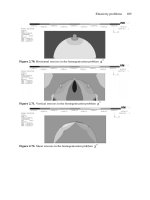
The results for the steady state analysis are shown in Figures 7.42 7.45 in the
form of a spatial temperature distribution and the analogous heat flux distribution
along the composite; their error approximations are computed and visualised also.
362 Computational Mechanics of Composite Materials
Considering the nonstationary character of the transient heat transfer, the
temperature distributions for various moments of the heating process are collected
in Figures 7.46 7.53. Analysing the temperatures fields along the composite
structure it can be observed that the best agreement with the structural behaviour is
obtained for the test related to the multiresolutionally homogenised composite. The
classical homogenisation method gives more accurate results in the neighbourhood
of the heated surface only. In the case of temperature gradients it can be concluded
that the wavelet based homogenisation approach gives the highest averages

temperature gradient and greater than the classical method and spatial averaging,
respectively. It is important considering reliability analysis based on the
homogenisation methods; this gradient is however a few percent smaller than the
maximum gradient for the real composite.
Figure 7.42. Spatial distribution of temperatures in composite
Figure 7.43. Temperature gradients along the composite
Multiresolutional Analysis 363
Figure 7.44. Solution error distribution along the composite
Figure 7.45. Temperature gradient error along the composite
364 Computational Mechanics of Composite Materials
Figure 7.46. Temperature distribution for t=2x10 E4 sec
Figure 7.47. Temperature distribution for t=4x10 E4 sec
Multiresolutional Analysis 365
Figure 7.48. Temperature distribution for t=5x10 E4 sec
Figure 7.49. Temperature distribution for t= 8x10 E4 sec
366 Computational Mechanics of Composite Materials
Figure 7.50. Temperature distribution for t= 4x10 E5 sec
Figure 7.51. Temperature distribution for t=6x10 E5 sec
Multiresolutional Analysis 367
Figure 7.52. Temperature distribution for t=8x10 E5 sec
Figure 7.53. Temperature distribution for t=1x10 E6 sec
The temperature solution error related to the real composite behaviour
numerical tests is best approximated by the error computed for the structure
homogenised by the wavelet based methodology also – it shows analogous spatial
distribution and maximum values, although spatial distribution is analogous in all
cases as well. In further analysis the results obtained should be contrasted with the
implementation of the wavelet decomposition of initial material properties in the
Finite Element Method program.
Finally, transient behaviour of the composite is analysed numerically and
presented for various time moments of the heating process in Figures 7.46 7.53.

The real composite is heated at the boundary relevant to the material with higher
volumetric heat capacity and the contrast between heat capacities is very high. That
is why the heating process in the real composite is very slow – significantly slower
than takes place in all homogenised models (Figure 7.53 corresponds to almost a
368 Computational Mechanics of Composite Materials
steady state for comparison). The opposite relation can be noticed in the case of
inverted materials in the analysed laminate. Neglecting temperature scale
differences between the real and effective models, the best approximation for the
original structure behaviour is done by the spatially averaged system.
7.7 Stochastic Perturbation based Approach to
the Wavelet Decomposition
Let us consider a multiresolutional wavelet based algorithm and its application
in the solution of the linear algebraic equations system [334] being a basis for
various discrete numerical techniques [206]. There holds
fKq =
(7.119)
where the matrix K is positive definite and represents the behaviour of some linear
engineering system, q is a discretised vector of the engineering system response
resulting from the excitation expressed by a vector f. Further, let us assume for the
needs of the algorithm applicability, that matrix K is of the size 2
n
x2
n
and let us
introduce the Haar transform for the vector q in the following way:
()
)2()12()(
2
1
kkk

qqs +=
−
(7.120)
()
)2()12()(
2
1
kkk
qqd −=
−
(7.121)
with k=1, ,2
n-1
. Let us observe that s
(k)
are introduced to scale averages of the
vector
q
values in the neighbouring points while
d
(k)
is to scale their differences.
Let us introduce the matrix M
n
such that
⎥
⎥
⎥
⎥
⎥

⎥
⎥
⎥
⎥
⎦
⎤
⎢
⎢
⎢
⎢
⎢
⎢
⎢
⎢
⎢
⎣
⎡
−
−
==







M
n
001100

0011
001100
0011
2
1
M
(7.122)
having dimensions 2
n
x2
n
and such that
Multiresolutional Analysis 369
IMMMM
T
nnn
T
n
==
(7.123)
whose top half is denoted by L
n
, while the bottom one is H
n
. Then, the
orthogonality gives
ILLHHMM
n
T
nn

T
nn
T
n
=+=
(7.124)
and
IHH
n
T
n
= , ILL
n
T
n
=
(7.125)
where
sLq = , dHq =
(7.126)
Let us rewrite (7.119) in the form of a pair of equations with unknown s and d
as follows:
(
)
(
)
LfHqLKHLqLKLLKq =+=
TT
(7.127)
Similarly, there holds

(
)
(
)
HfHqHKHLqHKLHKq =+=
TT
(7.128)
Denoting further by
CLKHTLKL ==
TT
,
(7.129)
and
AHKHBHKL ==
TT
,
(7.130)
as well as
ds
fHffLf == ,
(7.131)
we obtain (7.131) as
⎩
⎨
⎧
=+
=+
d
s
fAdBs

fCdTs
(7.132)