Mechanics of Materials 1 Part 3 ppsx

95.13
Slope and Deflection
of
Beams
123
Integrating again to find the deflection equation we have:
x2
a(T2-T,)
x2
d
'2
2
-+Cc,
Ely=
M +El
When
x
=
0,
y
=
0
.'.
C,
=
0,
and, since
M
=
-El
a(T2

then
y
=
0
for all values of
x.
d
Thus a rather surprising result is obtained whereby the beam will remain horizontal in the
presence
of
a thermal gradient. It will, however, be subject to residual stresses arising from the
constraint on overall expansion of the beam under the average temperature
+(T,
+
T2).
i.e. from
$2.3
residual stress
=
Ea[$(T,
+
T2)]
=
+Ea(T,
+T,).
(5.36)
Examples
Example
5.1
(a)

A
uniform cantilever is
4
m long and carries a concentrated load of
40
kN
at a point
3
m
from the support. Determine the vertical deflection of the free end of the cantilever if
EI
=
65
MN
m2.
(b) How would this value change if the same total load were applied but uniformly
distributed over the portion of the cantilever
3
m from the support?
Solution
(a) With the load in the position shown in Fig.
5.35
the cantilever is effectively only
3
m
long, the remaining
1
m being unloaded and therefore not bending. Thus, the standard
equations for slope and deflections apply between points
A

and
B
only.
WL~
40
x
103
x
33
Vertical deflection of
B
=
-
-
=
-
=
-
5.538
x
m
=
6,
3EI
3
x
65
x
lo6
WL~

40
x
103
x
32
Slope at
B
=
-
- -
=
2.769
x
rad
=
i
2El
2
x
65
x
lo6
Now
BC
remains straight since it is not subject to bending.
124
Mechanics
of
Materials

6,
=
-iL
=
-2.769
x
x
1
=
-2.769
x
lov3
m
vertical deflection
of
C
=
6,
+
6,
=
-
(5.538
+
2.769)10-3
=
-8.31
mm
The negative sign indicates a deflection in the negative

y
direction, i.e. downwards.
(b) With the load uniformly distributed,
40
x
103
=
13.33
x
lo3
N/m
w=-
3
Again using standard equations listed in the summary
wL4
8EI
13.33
x
lo3
x
34
8
x
65
x
lo6
6‘
-
= =
-2.076

x
m
1-
wL3
6EI
13.33
x
lo3
x
33
6
x
65
x
lo6
and slope
i
=
-
- -
=
0.923
x
lo3
rad

.’.
6;
=
-0.923

x x
1
=
0.923
x
10-3m
vertical deflection of
C
=
6;
+Si
=
-
(2.076+0.923)10-3
=
-
3mm
There is thus a considerable
(63.9%)
reduction in the end deflection when the load is
uniformly distributed.
Example
5.2
Determine the slope and deflection under the
50
kN
load for the beam loading system
E
=
200

GN/mZ;
I
=
83
x
lov6
m4.
shown in Fig.
5.36.
Find also the position and magnitude
of
the maximum deflection.
20
kN
lm + 2m+2m
R,=130
kN
-IX
Fig.
5.36.
Solution
Taking moments about either end
of
the beam gives
Ra=
6okN
and
RB=
130kN
Applying Macaulay’s method,

EI
d2y
10
dx
BMxx
=
j
7
=
6ox
-
20[(x
-
l)]
-
50[(x
-
3)l-
6o
The load unit of kilonewton is accounted for by dividing the left-hand side of
(1)
by
lo3
and
the u.d.1. term is obtained by treating the u.d.1. to the left of
XX as a concentrated load of
60(x
-
3)
acting at its mid-point

of
(x
-
3)/2
from XX.
Slope and Depection
of
Beams
125
Integrating
(l),
(2)
x
-
3)2
(x
-
3)3
103dx
El
dy
-
60x2 2
20
[
q]
-
50
[
+]

-
60
[
+
A
-
El
60x3 20[
v]
-
50[
71
(x
-
3)3
-
60[
!4]
x
-
3)4 +Ax
+
B
(3)
lo3
’-
6
and
Nowwhenx=O,
y=O

.‘.B=O
when
x
=
5,
y
=
0
.’.
substituting in
(3)
60x 20~4~ 50~2~ 60~2~
o= ~
+
5A
6 6 6 24
0
=
1250
-
213.3
-
66.7
-
40
+
5A

5A
=

-930
A
=
-186
Substituting
in
(2),

slope at
x
=
3
m (i.e. under the
50
kN load)
103 x 44
186
=
2
]
200 x
log
x 83 x
=
0.00265rad
And, substituting in
(3),
-
103
Y

=
~
-
20[
v]
-
50[
7 ]
(x
-
3)3
-
60[
!4]
x
-
3)4
-
186~
El
60 x
33
6
.’.
deflection at
x
=
3
m
186 x

31
103
60x33 20x23

___-___-
-,I[
6 6
103
lo3
x 314.7
-
[
270
-
26.67
-
5581
=
-
El
200 x 109 x 83 x
10-6
=
-0.01896m
=
-19mm
In order to determine the maximum deflection, its position must first
be
estimated. In this
case, as the

slope
is positive under the
50
kN
load it is reasonable to assume that the maximum
deflection point will occur somewhere between the
20
kN and
SO
kN loads. For this position,
from
(2),
El
dy
60~’ (x-1)’
103dx 2 2
-
20-
-
186
=
30~’
-
lox2
OX
-
10
-
186
=

20~’
+
20~
-
196
126
Mechanics
of
Materials
But, where the deflection is a maximum, the
slope
is zero.

0
=
20x2
+
20~
-
196
-
20
&
(400
+
15680)”2
-
20
126.8
-

-
40
40

X=
i.e.
x
=
2.67m
Then, from
(3),
the maximum deflection is given by
1
20
x 1.673
6
-
-
186
x
2.67
s,,,=

EI
=
-
0.0194
=
-
19.4mm

lo3 x 321.78
=-
200 109 x
83
x
10-6
In loading situations where this point lies within the portion of a beam covered by
a
uniformly distributed load the above procedure is cumbersome since it involves the solution
of
a
cubic equation to determine
x.
As
an alternative procedure it is possible to obtain
a
reasonable estimate
of
the position of
zero slope, and hence maximum deflection, by sketching the slope diagram, commencing with
the slope at either side
of
the estimated maximum deflection position; slopes will then be
respectively positive and negative and the point
of
zero slope thus may be estimated. Since the
slope diagram is generally a curve, the accuracy of the estimate is improved as the points
chosen approach the point of maximum deflection.
As
an example

of
this procedure we may re-solve the final part of the question.
Thus, selecting the initial two points as
x
=
2
and
x
=
3,
when
x
=
2,
186
=
-76
EZ
dy
60
x
22
20(12)
lo3
dx
2 2
when
x
=
3,

186
=
+44
EZ
dy
60~3~
20(22)
lo3
dx
2 2
=
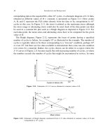
Figure
5.37
then gives a first estimate
of
the zero slope (maximum deflection) position as
x
=
2.63
on the basis
of
a straight line between the above-determined values. Recognising the
inaccuracy
of
this assumption, however, it appears reasonable that the required position can
/
I’

X
2

I
/\
3
Fig.
5.31.
Slope
and
Dejection
of
Beams
127
be more closely estimated as between
x
=
2.5
and
x
=
2.7.
Thus, refining the process further,
when
x
=
2.5,
El
dy
60~2.5~ 20x 1.5’
lo3
dx
2

2
- -
-186=
-21
when
x
=
2.7,
El
dy
60~2.7~
20x 1.72
lo3
dx
2 2
-
186
=
+3.8
-
-
Figure
5.38
then gives the improved estimate
of
x
=
2.669
which
is

effectively the same value as that obtained previously.
Fig.
5.38.
Example
5.3
Determine the deflection at a point
1
m from the left-hand end of the beam loaded as
shown in Fig.
5.39a
using Macaulay’s method.
El
=
0.65
MN m2.
20
kN
20
kN
t
B
!+6rn+I.2
m+1.2
m
Rb
la
1
20
kN
20

kN
x !
14kN
lb)
Fig.
5.39.
Solution
Taking moments about
B
(3
x
20)
+
(30
x
1.2
x
1.8)
+
(1.2
x
20)
=
2.4RA

RA=62kN
and
RB=20+(30x1.2)+20-62= 14kN
128
Mechanics

of
Materials
Using the modified Macaulay approach
for
distributed
loads
over part
of
a beam
introduced in
(j
5.5
(Fig. 5.39b),
[
-yl2
]
+
30[ -;.8'
]
-2O[(X
-
1.8),
El
d2y
lo3
dx2
M,,
= I
=
-

20~
+
62[
(X
-0.6)]
-
30
__
El
dy
-
-20x2 +62[
(X
-
0.6)2 ]-30[(
x
-
0.6)3
]+30[(
x
-
1.8)3
]
103
dx
2
EI
-
2oX3 +62[
(X

-
0.6)3 ]-~O[(~-O.~)'
mY=6
24
(X
-
1.8)'
+
30[ 24
-20[
6
(X
-
1.8)3
+A
+AX+B
Now when
x
=
0.6,
y
=
0,
20
x
0.63

o=
-
+

0.6A
+
B
6
0.72
=
0.6A
+
B
y
=
0,
20
x
33 62
x
2.43 30
x
2.4' 30
x
1.2' 20
x
l.z3
and when x
=
3,
+

o=
-___

-
+3A+B
6 24 24 6
+
-
6
=
-
90
+
142.848
-
41.472
+
2.592
-
5.76
+
3A
+
B
-
8.208
=
3A
+
B
(2)
-
(1)

-
8.928
=
2.4A
.'.
A
=
-3.72
Substituting in
(l),
B
=
0.72 -0.6(
-
3.72)
B
=
2.952
Substituting into the Macaulay deflection equation,
SY
El
=
-~
20x3
+
62[
('
-:6)3
]
-

30[
(x
t6)"]
+
30[
(x
;-')'I
6
-
20
[
(x
-:'8'9
1
-
3.72~
+
2.952
At
x=l
1
30
x
0.4'
24
-
3.72
x
1
+

2.952
20 62
66
+
-
x
0.43
-
Slope
and Defection
of
Beams
129
103
=
-
[
-
3.33
+
0.661
-
0.032
-
3.72
+
2.9521
El
=
-5.34~ i0-3m

=
-5.34mm
lo3
x
3.472
0.65
x
lo6
=-
The beam therefore is deflected
downwards
at the given position.
Example
5.4
from the left-hand end.
E1
=
1.4MNm2.
Calculate the slope and deflection of the beam loaded as shown in Fig. 5.40 at a point 1.6
m
30,
kN
7
20kN
30
kN
+-
I6
m
-07m-/

I
I
5
7kNm
-+’I3
kN
m
for
B.M.
20kN diagram load
06x
13
l3=6kNm~
2
X
Fig.
5.40.
Solution
Since,
by
symmetry, the point
of
zero
slope
can be located at C a solution can
be
obtained
conveniently using Mohr’s method. This is best applied by drawing the B.M. diagrams for the
separate effects of (a) the 30 kN loads, and (b) the 20 kN load as shown in Fig. 5.40.
Thus, using the zero slope position C as the datum for the Mohr method, from eqn. (5.20)

1
E1
slope at
X
=
-
[area of B.M. diagram between
X
and C]
103
=
~
[
(
-
30
x
0.7)
+
(6
x
0.7)
+
(3
x
7
x
0.7)]
EI
103 14.35 x

lo3
EI
1.4 x
lo6
=-[-21+4.2+2.45]
=
-
=
-
10.25 x 1O-j rad
and from eqn. (5.21)
130
Mechanics
of
Materials
deflection at
X
relative to the tangent at
C
1
El
-

[first moment
of
area
of
B.M.
diagram between
X

and
C
about
X]
103
6,yc
=
__
[
(
-
30
x
0.7
x
0.35)
+
(6
x
0.7
x
0.35)
+
(7
x
0.7
x
3
x
3

x
0.7)]
A,%
A222
'43%
El
103
103
x
4.737
=
[
-
7.35
+
1.47
+
1.1431
=
-
El
1.4
x
lo6
=
-3.38
x
10-3m
=
-3.38mm

This must now be subtracted from the deflection
of
C
relative to the support
B
to obtain the
actual deflection at
X.
Now
deflection
of
C
relative to
B
=
deflection
of
B
relative to
C
1
El
=
-
[first moment
of
area
of
B.M.
diagram between

B
and
C
about
B]
103
=-[(-30~1.3~0.65)+(13~1.3~~~1.3~~)]
El
=
-
12.88
x
=
-
12.88mm
103
18.027
x
lo3
El
1.4
x
lo6
=
-
[
-
25.35
+
7.3231

=
-
.'.
required deflection
of
X
=
-
(12.88
-
3.38)
=
-
9.5
mm
Example
5.5
(a) Find the slope and deflection at the tip
of
the cantilever shown in Fig.
5.41.
20
kN
A
B
Bending moment
diagrams
I
I
la)

20
kN
laad
at
end
(c)Upward load
P
2P
Fig.
5.41
Slope
and
Deflection
of
Beams
131
(b) What load
P
must be applied upwards at mid-span to reduce the deflection by half?
EI
=
20
MN mz.
Solution
Here again the best approach is
to
draw separate B.M. diagrams for the concentrated and
uniformly distributed loads. Then, since
B
is a point of zero

slope,
the Mohr method may be
applied.
1
EI
(a) Slope at
A
=
-[area of B.M. diagram between
A
and
B]
1
103
=-[A,
+A,]
= [{$
x
4
x
(-80))
+{fx
4
x
(-
160)}]
El
EI
103
373.3

x
103
=-[-160-213.3]
=
EI
20
x
lo6
=
18.67 x
lo-’
rad
1
EI
Deflection
of
A
=
-
[first moment of area
of
B.M. diagram between
A
and
B
about
A]
lo3
[
(

-
80
x
4
x
3
x
4)
+
(
-
160
x
4
x
3
x
4
El
2
-
103 1066.6
x
lo3
3
=
-53.3
x
w3rn
=

-53mm
=-
20
x
106
=-
[426.6+640]
=
-
EI
(b) When an extra load
P
is
applied upwards at mid-span its effect on the deflection is
required to
be
3
x
53.3
=
26.67
mm. Thus
1
EI
26.67
x
=
-
[first moment of area af-B.M. diagram for
P

about
A]
103
=
-
[+
x
2P
x
2(2+f
x
2)]
EI
26.67
x
20
x
lo6
lo3
x
6.66
P=
=BOX
103~

The required load at mid-span is
80
kN.
Example
5.6

The uniform beam
of
Fig.
5.42
carries the
loads
indicated. Determine the B.M. at
B
and
hence draw the
S.F.
and B.M. diagrams for the beam.
132
Mechanics
of
Materials
-:
“8“
30k
Total
0.M
diagrorn
LFrxmg moment dlagrom
Free moment diagrams
491
kN
-70
9-kN
Fig.
5.42.

Solution
Applying the three-moment equation
(5.24)
to the beam we have,
(Note that the dimension
a
is always to the “outside” support of the particular span carrying
the concentrated load.)
Now with
A
and
C
simply supported
MA=Mc=O

-
8kf~
=
(120+ 54.6)103
=
174.6
X
lo3
MB
=
-
21.8
kNm
With the normal
B.M.

sign convention the
B.M.
at
B
is therefore
-
21.8
kN m.
Taking moments about
B
(forces to left),
~RA
-
(60
X
lo3
X
2
X
1)
=
-
21.8
X
lo3
RA
=
+(
-
21.8

+
120)103
=
49.1
kN
Taking moments about
B
(forces to right),
2Rc
-
(50
x
lo3
x
1.4)
=
-
21.8
x
lo3
Rc
=
*(
-21.8
+
70)
=
24.1
kN
Slope and Defection

of
Beams
-3.39kN
133
24
kN
-
and, since the total load

=RA+RB+Rc=~O+(~OX~)=
170kN
RB
=
170-49.1 -24.1
=
96.8kN
The B.M. and S.F. diagrams are then as shown in Fig. 5.42. The fixing moment diagram can
be
directly subtracted from the free moment diagrams since MB is negative. The final B.M.
diagram is then as shown shaded, values at any particular section being measured from the
fixing moment line as datum,
e.g.
B.M.
at
D
=
+h
(to scale)
Example
5.7

A
beam
ABCDE
is continuous over four supports and carries the loads shown in Fig. 5.43.
Determine the values of the fixing moment at each support and hence draw the S.F. and B.M.
diagrams for the beam.
20
kN
10
kN
I
kN/m
A
A13.3
kN m
diagram
Solution
By inspection, MA
=
0
and MD
=
-
1
x
10
=
-
10
kNm

Applying the three-moment equation for the first two spans,
-
16MB- 3Mc
=
(31.25
+
53.33)103
-
16MB- 3Mc
=
84.58
x
lo3
134
Mechanics
of
Materials
and, for the second and third spans,
4
-3M~-2Mc(3+4)-(-10~10
-
~MB- 14Mc
+
(40
x
lo3)
=
(66.67
+
48)103

-
3MB- 14Mc
=
74.67
x
lo3
(2)
x
16/3
(3)
-
(1)
-
16MB- 74.67Mc
=
398.24
x
lo3
-
71.67Mc
=
313.66
x
lo3
Mc
=
-
4.37
x
lo3

Nm
Substituting in (l),
-
16~,
-
3(
-
4.37
x
103)
=
84.58
x
103
(84.58
-
13.11)103
16
Mg=
-
=
-
4.47 kN
m
Moments about
B
(to left),
5R,
=
(-4.47

+
12.5)103
RA
=
1.61 kN
Moments about
C
(to left),
RAx8-(1
x103x5x5.5)+(R,x3)-(20x103x
1)= -4.37~
lo3
3R,
=
-
4.37
x
lo3
+
27.5
x
lo3
+
20
x
lo3
-
8
x
1.61

x
lo3
3R,
=
30.3
x
lo3
RE
=
10.1 kN
Moments about
C
(to right),
(-
IOX
lo3
x
5)+4RD-(3
x
lo3
x
4
x
2)
=
-4.37
x
lo3
4R,
=

(
-
4.37
+
50
+
24)103
R,
=
17.4 kN
Then, since
RA
+
R,
+
R,+ R,
=
47kN
1.61
+
10.1
+
R,+ 17.4
=
47
R,
=
17.9
kN
Slope

and
Defection
of
Beams
135
This value should then be checked by taking moments to the right of
B,
(
-
10
x
lo3
x
8)
+
7R,
+
3R,
-
(3
x
lo3
x
4
x
5)
-
(20
x
lo3

x
2)
=
-
4.47
x
lo3
3R,= (-4.47+40+60+80-
121.8)103
=
53.73
x
lo3
R,
=
17.9
kN
The
S.F.
and
B.M.
diagrams for the beam are shown in Fig.
5.43.
Example
5.8
Using the finite difference method, determine the central deflection of a simply-supported
over its complete span. The beam can be
beam carrying a uniformly distributed load
assumed to have constant flexural rigidity
El

throughout.
Solution
w
/
metre
A
E
Uniformly loaded
beam
Fig.
5.44.
As
a simple demonstration of the finite difference approach, assume that the beam is
divided into only four equal segments (thus reducing the accuracy of the solution from that
which could be achieved with a greater number of segments).
Then,
but, from eqn.
(5.30):
WL
L WL L 3WL2
2
4
48
32
B.M.
at
B
=
-
x

=
-
-
-
MB
and, since
y,
=
0,
3WL2
512
El

-
Yc
-
2YB.
136
Mechanics
of
Materials
Similarly
OL
L
OL
L
wL2
22
24

8
B.M.
at
C
=

-

=
-
- -
M,.
and, from eqn.
(5.30)
1
___
;!
(
y)
=
(L/4)2
(
YB
-
2YC
+
Y,)
Now, from symmetry,
y,
=

y,

wL4
128EI

-
2YB
-
2Yc
Adding eqns.
(1)
and
(2);
wL4
30L4
-yc=-+-
128EI 512EI
-
70L4
OL4
yc
=
~
=
-0.0137-
512EI
El

the negative sign indicating a downwards deflection as expected. This value compares with
the "exact" value of:

5wL4
OL4
yc=
- -
0.01302
-
384EI
El
a difference of about
5
%.
As stated earlier, this comparison could
be
improved by selecting
more segments but, nevertheless, it is remarkably accurate for the very small number of
segments chosen.
Example
5.9
The statically indeterminate propped cantilever shown in Fig.
5.45
is propped at Band carries
a central load
W
It can be assumed to have a constant flexural rigidity
El
throughout.
Fig.
5.45
Slope
and Defection

of
Beams
137
Determine, using a finite difference approach, the values of the reaction at the prop and the
central deflection.
Solution
Whilst at first sight, perhaps, there appears to be a number of redundancies in the cantilever
loading condition, in fact the problem reduces
to
that of a single redundancy, say the
unknown prop load
P,
since with a knowledge of
P
the other “unknowns”
MA
and
R,
can be
evaluated easily.
Thus, again for simplicity, consider the beam divided into four equal segments giving three
unknown deflections
yc, y,
and
yE
(assuming zero deflection at the prop
B)
and one
redundancy. Four equations are thus required for solution and these may be obtained by
applying the difference equation at four selected points on the beam:

From eqn.
(5.30)
PL
El
B.M. at
E
=
M
=- =-
(YB-~YE
+
YO)
E
4 (L/4)2
but
y,
=
0
But
yA
=
0

3L
WL
El
B.M. at
C
=
Mc

=
P
-
-
=
-
(
Y,
-
2YC
+
YD)
4 4 (L/4)2
3PL3
m3
y,- 2yc
=
-
-
-
6464
(3)
At point
A
it is necessary to introduce the mirror image of the beam giving point
C’
to the left
of
A
with a deflection

y;
=
yc
in order to produce the fourth equation.
Then:
and again since
y,
=
0
PL3
WL3
yc=
32
64
Solving equations
(1)
to
(4)
simultaneously gives the required prop load:
7w
P
=
=
0.318
W,
LL
and the central deflection:
(4)
17W3
wz3

y
= =
-0.0121-
1408EI
El
138
Mechanics
of
Materials
Problems
5.1 (AD). A
beam of length 10m is symmetrically placed on two supports 7m apart. The loading is 15 kN/m
between the supports and 20kN at each end. What is the central deflection of the
beam?
E
=
210GN/mZ;
I
=
200
x 10-6m4.
[6.8 mm.]
5.2 (A/B).
Derive the expression for the maximum deflection of a simply supported
beam
of negligible weight
carrying a point load at its mid-span position. The distance between the supports is
L,
the second moment of area
of

the cross-section is
I
and the modulus of elasticity
of
the beam material is
E.
The maximum deflection of such
a
simply supported beam of length 3 m is 4.3 mm when carrying a
load
of 200 kN
at its mid-span position. What would be the deflection at the free end ofacantilever
of
the same material, length and
cross-section if it carries a load
of
l00kN at a point 1.3m from the free end?
[
13.4
mm.]
5.3 (AD). A
horizontal
beam,
simply supported at its ends, carries a load which varies uniformly from
15
kN/m
at one end to 60 kN/m at the other. Estimate the central deflection if the span is 7 m, the section 450mm deep and the
maximum bending stress 100MN/m2.
E
=

210GN/mZ.
[U.L.] [21.9mm.]
5.4
(A/B). A
beam AB,
8
m long, is freely supported
at
its ends and carries loads of 30 kN and
50
kN at points 1 m
and
5
m respectively from
A.
Find the position and magnitude of the maximum deflection.
E
=
210GN/m2;
I
=
200
x 10-6m4.
[
14.4 mm.]
5.5 (A/B). A
beam
7
m long is simply supported
at

its ends and loaded as follows: 120 kN at 1
m
from one end
A,
20 kN at 4
m
from
A
and 60 kN at
5
m from
A.
Calculate the position and magnitude of the maximum deflection. The
second moment of area of the beam section is
400
x
[9.8mm at 3.474m.l
5.6 (B). A
beam ABCD, 6 m long, is simply-supported at the right-hand end
D
and at
a
point
B
1 m from the left-
hand end A. It carries a vertical load of 10 kN at A,
a
second concentrated load of 20 kN at C, 3 m from
D,
and

a
uniformly distributed load of 10 kN/m between C and
D.
Determine the position and magnitude of the maximum
deflection if
E
=
208 GN/mZ and
1
=
35 x
C3.553 m from
A,
11.95 mm.]
5.7
(B). A
3
m long cantilever ABCis built-in at
A,
partially supported at
B,
2 m from
A,
with a force
of
10
kN and
carries
a
vertical load of 20 kN at C.

A
uniformly distributed load of
5
kN/m is also applied between
A
and
B.
Determine a) the values of the vertical reaction and built-in moment at
A
and b) the deflection of the free end C of the
cantilever.
Develop an expression for the slope of the beam at any position and hence plot a slope diagram.
E
=
208 GN/mz
and
I
=
24 x m4. [ZOkN, SOkNm, -15mm.l
5.8 (B).
Develop a general expression for the slope of the beam of question
5.6
and hence plot
a
slope diagram for
the beam. Use the slope diagram to confirm the answer given in question 5.6 for the position of the
maximum
deflection of the beam.
5.9 (B).
What would be the effect on the end deflection for question 5.7, if the built-in end

A
were replaced by a
simple support at the same position and point
B
becomes
a
full simple support position (i.e. the force at
B
is no longer
10
kN). What general observation can you make about the effect of built-in constraints on the stiffness of beams?
C5.7mm.l
5.10 (B). A
beam AB is simply supported
at
A
and
B
over a span of 3 m. It carries loads of 50kN and 40kN at
0.6m and 2m respectively from
A,
together with
a
uniformly distributed load of
60
kN/m between the 50kN and
40 kN concentrated loads. If the cross-section of the beam is such that
1
=
60

x m4 determine the value of the
deflection of the beam under the 50kN load.
E
=
210GN/m2. Sketch the S.F. and B.M. diagrams for the
beam.
13.7 mm.]
5.11 (B).
Obtain the relationship between the
B.M.,
S.F., and intensity of loading of
a
laterally loaded beam.
A
simply supported beam
of
span
L
carries a distributed load of intensity kx2/L2 where
x
is measured from one
(a) the location and magnitude of the greatest bending moment;
(b) the support reactions.
[
U.Birm.1 [0.63L, 0.0393kLZ, kL/12, kL/4.]
5.12 (B). A
uniform
beam
4m long is simplx supported at its ends, where couples are applied, each 3 kN m in
m4

determine the magnitude of the
What load must be applied at mid-span to reduce the deflection by half? C0.317 mm, 2.25 kN.]
5.13
(B).
A
500mm xJ75mmsteelbeamoflength
Smissupportedattheleft-handendandatapoint
1.6mfrom
the right-hand end.
The
beam
carries
a
uniformly distributed load of 12 kN/m on its whole length, an additional
uniformiy distributed load of 18 kN/m on the length between the supports and a point load of 30 kN at the right-
hand end. Determine the
slope
and deflection of the beam at the section midway between the supports and also at the
right-hand end.
El
for the beam is
1.5
x 10' NmZ. [U.L.] C1.13 x 3.29mm, 9.7 x 1.71 mm.]
m4 and
E
for the beam material is 210GN/m2.
m4.
support towards the other. Find
magnitude but opposite in sense.
If

E
=
210GN/m2 and
1
=
90
x
deflection at mid-span.
Slope
and
Defection
of
Beams
139
5.14
(B).
A
cantilever, 2.6 m long, carryinga uniformly distributed load
w
along the entire length, is propped at its
free end to the level of the fixed end.
If
the load on the prop is then 30 kN, calculate the value of
w.
Determine also
the
slope
of the beam at the support. If any formula
for
deflection is used it must first be proved.

E
=
210GN/m2;
I
=
4
x
10-6m4.
[U.E.I.] C30.8 kN/m, 0.014 rad.]
5.15
(B).
A
beam
ABC
of total length
L
is simply supported at one end
A
and at some point
B
along its length. It
carriesa uniformly distributed load
of
w
per unit length over its whole length. Find the optimum position
of
B
so
that
the greatest bending moment in the beam is as low

as
possible.
[U.Birm.] [L/2.]
m4, is hinged at
A
and simply
supported on a non-yielding support at
C.
The beam is subjected to the given loading (Fig. 5.46).
For
this loading
determine (a) the vertical deflection of
E;
(b) the slope of the tangent to the bent centre line at
C.
E
=
80GN/m2.
[I.Struct.E.] [27.3mm, 0.0147 rad.]
5.16
(B).
A
beam
AB,
of constant section, depth 400 mm and
I,,
=
250
x
x)

kN/rn
1”
kN
1
I
Fig. 5.46.
5.17
(B).
A
simply supported beam
AB
is 7 m long and carries a uniformly distributed load of 30 kN/m run.
A
couple is applied to the beam at a point
C,
2.5m from the left-hand end,
A,
the couple being clockwise in sense and of
magnitude 70 kNm. Calculate the slope and deflection of the beam at a point
D,
2 m from the left-hand end. Take
EI
=
5
x.
lo7 Nm’. [E.M.E.U.] C5.78
x
10-3rad, 16.5mm.l
5.18
(B).

A
uniform horizontal beam
ABC
is 0.75
m
long and is simply supported at
A
and
B,
0.5 m apart, by
supports which can resist upward or downward forces.
A
vertical load of 50N is applied at the free end
C,
which
produces a deflection of
5
mm at the centre
of
span
AB.
Determine the position and magnitude
of
the maximum
deflection in the span
AB,
and the magnitude of the deflection at
C.
.[E.I.E.] C5.12 mm (upwards), 20.1 mm.]
5.19

(B).
A
continuous beam
ABC
rests on supports at
A, B
and
C.
The portion
AB
is 2m long and carries
a
central concentrated load of40 kN, and
BC
is 3
m
long with a u.d.1. of
60
kN/m on the complete length. Draw the S.F.
and B.M. diagrams for the beam.
[
-
3.25, 148.75, 74.5 kN (Reactions);
M,
=
-
46.5
kN m.]
5.20
(B). State Clapeyron’s theorem of three moments.

A
continuous beam
ABCD
is
constructed of built-up
sections whose effective flexural rigidity
El
is constant throughout its length.
Bay
lengths are
AB
=
1
m,
BC
=
5
m,
CD
=
4 m. The beam is simply supported at
B,
C
and
D,
and carries point loads of 20 kN and 60 kN at
A
and midway
between
C

and
D
respectively, and
a
distributed load
of
30kN/m over
BC.
Determine the bending moments and
vertical reactions at the supports and sketch the B.M. and
S.F.
diagrams.
CU.Birm.1 [-20, -66.5, OkNm; 85.7, 130.93, 13.37kN.l
5.21
(B).
A
continuous beam
ABCD
is simply supported over three spans
AB
=
1 m,
BC
=
2 m and
CD
=
2 m.
The first span carries a central load
of

20 kN and the third span a uniformly distributed load of 30 kN/m. The central
span remains unloaded. Calculate the bending moments at
B
and
C
and draw the
S.F.
and B.M. diagrams. The
supports remain at the same level when the beam is loaded.
[1.36, -7.84kNm; 11.36, 4.03, 38.52, 26.08kN (Reactions).]
5.22
(B).
A
beam, simply supporded at its ends, carries a load which increases uniformly from
15
kN/m at the left-
hand end to 100 kN/m at the right-hand end. If the beam is
5
m long find the equation for the rate of loading and,
using this, the deflection
of
the beam at mid-span if
E
=
200GN/m2 and
I
=
600
x
10-6m4.

[w
=
-
(1
5
+
85x/L); 3.9 mm.]
5.23
(B).
A
beam
5
m long is firmly fixed horizontally at one end and simply supported at the other by a prop. The
beam carries
a
uniformly distributed load of 30 kN/m run over its whole length together with a concentrated load of
60 kN at a point 3 m from the fixed end. Determine:
(a) the load carried by the prop if the prop remains at the same level as the end support;
(b) the position of the point of maximum deflection.
[B.P.] [82.16kN; 2.075m.l
5.24
(B/C).
A
continuous beam
ABCDE
rests on five simple supports
A, B, C,
D
and
E.

Spans
AB
and
BC
carry a
u.d.1.
of
60 kN/m and are respectively 2 m and 3 m long.
CD
is 2.5 m long and carries a concentrated load of
50
kN at
1.5 m from
C.
DE
is 3 m long and carries a concentrated load of
50
kN at the centre and a u.d.1. of 30 kN/m. Draw the
B.M. and
S.F.
diagrams for the beam.
[Fixing moments:
0,
-44.91, -25.1, -38.95, OkNm. Reactions: 37.55, 179.1, 97.83, 118.5, 57.02kN.l
CHAPTER
6
BUILT-IN BEAMS
Summary
The
maximum bending moments and maximum deflections for built-in beams with

standard loading cases are as follows:
MAXIMUM B.M. AND DEFLECTION FOR BUILT-IN BEAMS
Loading case
Central concentrated
load W
Uniformly distributed
load w/metre
(total load
W)
Concentrated load W
not at mid-span
Distributed load w’
varying in intensity
between x
=
x, and
x
=
x2
Maximum B.M.
WL
8
-
wL2 WL
12 12
_-

Wab2 Wa2b
~
or

-
L2
L2
w‘(L -x)Z
MA=
-
dx
Maximum deflection
WL3
192EI
__
wL4 WL3
38481 384EI
__=-
2 Wa3b2 2aL
at x=-
(L
+
2a)
3EI(L
+
2a)2
where a
<
-
Wa3b3
3EIL3
=-
under load
140

$6.1
Built-in Beams
141
Efect
of
movement
of
supports
If one end
B
of an initially horizontal built-in beam
AB
moves through a distance
6
relative
to end
A,
end moments are set up of value
and the reactions at each support are
Thus, in most practical situations where loaded beams sink at the supports the above values
represent
changes
in fixing moment and reaction values, their directions being indicated in
Fig. 6.6.
Introduction
When both ends of
a
beam are rigidly fixed the beam is said to be
built-in, encastred
or

encastri.
Such beams are normally treated by a modified form of Mohr’s area-moment
method or by Macaulay’s method.
Built-in beams are assumed to have zero slope at each end,
so
that the total change of slope
along the span is zero. Thus, from Mohr’s first theorem,
M.
El
area of
-
diagram across the span
=
0
or, if the beam is uniform,
El
is constant, and
area
of
B.M. diagram
=
0
(6.1)
Similarly, if both ends are level the deflection of one end relative to the other is zero.
Therefore, from Mohr’s second theorem:
M
EI
first moment of area of
-
diagram about one end

=
0
and, if
EZ
is constant,
first moment
of
area
of
B.M. diagram about one end
=
0
(6.2)
To make use of these equations it is convenient to break down the B.M. diagram for the
(a) that resulting from the loading, assuming simply supported ends, and known as the
(b) that resulting from the end moments or fixing moments which must
be
applied at the
built-in beam into two parts:
free-moment diagram;
ends to keep the slopes zero and termed the
fixing-moment diagram.
6.1.
Built-in beam carrying central concentrated load
Consider the centrally loaded built-in beam of Fig. 6.1.
A,
is the area of the free-moment
diagram and
A,
that of the fixing-moment diagram.

142
Mechanics
of
Materials
46.2
iA-
Free' ment diagram
Fixing moment diagmm
%I1
M=-%
8
Fig.
6.1.
By symmetry the fixing moments are equal at both ends. Now from eqn.
(6.1)
A,+&
=
0

WL
3
x
LX
-=
-ML
4
The B.M. diagram is therefore as shown in Fig.
6.1,
the maximum B.M. occurring at both the
ends and the centre.

Applying Mohr's second theorem for the deflection at mid-span,
first moment
of
area
of
B.M. diagram between centre and
one end about the centre
6=[
1L ML L
1
[
WL~
ML~
1
WL~ WL~
EZ
96
8
El
96
(i.e. downward deflection)
WLJ
192EZ
-

-
6.2.
Built-in beam carrying uniformly distributed load across the span
Consider now the uniformly loaded beam of Fig.
6.2.

$6.3
Built-in
Beams
143
'Free' moment diagram
I
I
Fixing moment diagram
Ab1Z-d
12
I
I
Fig.
6.2.
Again, for zero change of slope along the span,
&+A,
=
0

2
WL2
-x- xL=-ML
38
The deflection at the centre is again given by Mohr's second theorem as the moment of one-
half of the B.M. diagram about the centre.

6
=
[
(3

x
$
x
;)(;
x
;)+
(y
x
$)]A
EI
wL4
384
E
I
The negative sign again indicates a downwards deflection.
-
-

6.3.
Built-in beam carrying concentrated load offset from the centre
Consider the loaded beam of Fig.
6.3.
Since the slope at both ends is zero the change
of
slope across the span is zero, i.e. the total
area between
A
and
B
of

the B.M. diagram is zero (Mohr's theorem).
144
Mechanics
of
Materials
46.3

L
Fig.
6.3.
Also
the deflection of
A
relative to
B
is zero; therefore the moment
of
the
B.M.
diagram
between
A
and
B
about
A
is
zero.

[~x~xa]~+[jxt wabxb

I(
a+-
:)
+
(
+MALx-
4)
+
(
+MBLx-
't)
=O
Wab
MA+2M~=
-
[2a2+3ab+b2]
L3
Subtracting
(l),
Wab
L3
M
-
-
-[2a2
+
3ab+ b2
-
L2]
8-

but
L=a+b,
Wab
L3
M
[2a2
+
3ab
+
bZ
-
a2
-
2ab
-
b2]
B-

Wab Wa'bL
[a
+ab]
=
-___
L3 L3
=
-__
56.4
Built-in Beams
145
Substituting in (l),

Wab Wa2b
L
L2
M
+-
A-
Wab(a
+
b) Wa2b
=-
+-
Wab’
LZ
L2
L2
=
-__
6.4.
Built-in beam carrying a non-uniform distributed load
Let
w’
be
the distributed load varying in intensity along the beam as shown in Fig. 6.4. On a
short length
dx
at a distance
x
from
A
there is a load of

w’dx.
Contribution
of
this load to
MA
Wab2
=
-~
L2
(where
W
=
w’dx)
w’dx
x
x(L
-
x)’
L2
1
w’x( L;x)’dx
-

total
MA
=
-
0
w’/me
tre

\
Fig.
6.4. Built-in
(encostre)
beam carrying non-uniform distributed load
Similarly,
(6.9)
(6.10)
0
If the distributed load is across only part
of
the span the limits
of
integration must
be
changed to take account
of
this: i.e. for a distributed load
w’
applied between
x
=
xl
and
x
=
x2
and varying in intensity,
(6.1 1)
(6.12)

146
Mechanics
of
Materials
$6.5
6.5.
Advantages and disadvantages
of
built-in beams
Provided that perfect end fixing can
be
achieved, built-in beams carry smaller maximum
B.M.s (and hence are subjected to smaller maximum stresses) and have smaller deflections
than the corresponding simply supported beams with the same loads applied; in other words
built-in beams are stronger and stiffer. Although this would seem to imply that built-in beams
should be used whenever possible, in fact this is not the case in practice. The principal reasons
are as follows:
(1)
The need for high accuracy in aligning the supports and fixing the ends during erection
(2)
Small subsidence of either support can set up large stresses.
(3)
Changes of temperature can also set up large stresses.
(4)
The end fixings are normally sensitive to vibrations and fluctuations in B.M.s, as in
These disadvantages can be reduced, however, if hinged joints are used at points on the
beam where the B.M. is zero, i.e. at
points
of
inflexion

or
contraflexure.
The beam is then
effectively a central beam supported on two end cantilevers, and for this reason the
construction is sometimes termed the
double-cantilever
construction. The beam
is
then free to
adjust to changes in level of the supports and changes in temperature (Fig.
6.5).
increases the cost.
applications introducing rolling loads (e.g. bridges, etc.).
oints
of
inflexion
Fig.
6.5.
Built-in
beam
using “doubleantilever” construction.
6.6.
Effect
of
movement
of
supports
Consider a beam
AB
initially unloaded with its ends at the same level. If the slope is to

remain horizontal at each end when
B
moves through a distance
6
relative to end
A,
the
moments must be as shown in Fig.
6.6.
Taking moments about
B
RA
x
L
=
MA+ MB
MA= Mg= M
and, by symmetry,
2M
L

RA=-
Similarly,
2M
L
RB=-
in the direction shown.
$6.6
Built-in
Beams

147
-M
Fig.
6.6.
Effect
of
support
movement
on
B.M.s.
Now from Mohr’s second theorem the deflection of
A
relative to
B
is equal to the first
moment
of
area of the B.M. diagram about
A
x
l/EI.

12EIS
and
RA=Re=-
6E1S
M=
L2
L3
(6.14)

in the directions shown in Fig.
6.6.
beam under load when one end sinks relative to the other.
These values will
also
represent the
changes
in the fixing moments and end reactions for
a
Examples
Example
6.1
An encastre beam has a span
of
3
m and carries the loading system shown in Fig.
6.7.
Draw
the B.M. diagram
for
the beam and hence determine the maximum bending stress set up. The
beam can be assumed to be uniform, with
I
=
42
x
m4 and with an overall depth
of
200
mm.

Solution
Using the
principle ofsuperposition
the loading system can
be
reduced to the three cases for
which the
B.M.
diagrams have been drawn, together with the fixing moment diagram, in
Fig.
6.7.