Modeling and Simulation for Material Selection and Mechanical Design Part 10 potx
Bạn đang xem bản rút gọn của tài liệu. Xem và tải ngay bản đầy đủ của tài liệu tại đây (1.14 MB, 23 trang )
Figure 42 Continued
Copyright 2004 by Marcel Dekker, Inc. All Rights Reserved.
The estimation of the rate of growth of such microcracks can be
achieved mainly by two methods: (a) the determination of the statistical dis-
tribution of the microcrack length and its variation with the creep time, and
(b) finite-element simulation of the creep behavior regarding the material as
a composite consisting of grains separated by thin grain boundary layer with
different properties.
1. Statistical Model
The fundamental concept of the statistical model is that a small fraction of
short cracks and a high fraction of long cracks are expected when the
growth rate is high, and vice versa [95–98]. In order to achieve reliable
results using statistics, a great number of cracks have to be classified. Over
a period of several years, about 50,000 cracks were classified in the steel X6
CrNi18-11 and more than 60,000 cracks in the steel X8CrNiMoNb16-16 for
different temperatures and stresses.
Based on the results of metallographic investigations, the following
assumptions are introduced: (a) A crack grows quickly along the grain
boundary from one triple point to the next, where it rests for a longer time
before it grows again to the next triple point, (b) The crack length is always
an integral multiple n of grain boundary facets and (c) every crack is
initiated in the length class n ¼ 1 and grows step by step to next higher
length classes.
Let Z be the total number of cracks per unit area and Y
n
the number of
cracks having a length n. In a time unit, V
n,n þ 1
cracks grow out of the
length class n into the next higher length class (n þ 1). In the same time,
V
n À 1,n
cracks grow from the lower length class (n À 1) into the considered
class n. The mean rate of growth is given by dn=d t ¼ V
n;nþ1
=Y
n
and the rate
of change of dY
n
=dt ¼ V
n;nþ1
À V
nÀ1;n
. As all cracks initiate with the length
n ¼ 1, the rate V
0;1
represents the rate of crack initiation and must be equal
to rate dZ=dt of the increase of the total crack number. Therefore, following
relation can be deduced:
V
n;nþ1
¼
dZ
dt
À
X
n
i¼1
dY
i
dt
ð86Þ
Denoting the fraction of cracks with the length of n by X
n
, so that
dY
n
¼ X
n
dZ þ ZdX
n
, the mean rate of growth ðdn=dtÞ
n
of the cracks of
the length class n can be written as
dn
dt
n
¼
1 À
P
n
i¼1
X
i
X
n
1
Z
dZ
dt
À
1
X
n
X
n
i¼1
dX
i
dt
!
¼ FðnÞGðtÞÀHðn; tÞ
ð87Þ
Copyright 2004 by Marcel Dekker, Inc. All Rights Reserved.
The first term denoted F(n) is determined by the statistical distribution of
the microcrack length. This distribution can be described by
X
n
¼ð1 ÀqÞq
nÀ1
ð88Þ
as represented in Fig. 43 for two different austenitic steels. Deviations are
mainly observed in the range of long microcracks and low population. These
deviations can be avoided by adding a second term including a Leibnitz
series, but it will be neglected here.
The function FðnÞ is then given by
F ¼
q
1 Àq
ð89Þ
The parameter q depends on stress, temperature, and the constitution
of the material, but not on crack length. Therefore, approximately no influ-
ence of the crack length on the growth rate arises from this term.
The function G, which is the relative rate of crack initiation, depends
on the material and the creep conditions. In order to determine this func-
Figure 43 Statistical distribution of the inter-crystalline creep microcracks.
Copyright 2004 by Marcel Dekker, Inc. All Rights Reserved.
tion, several creep tests are to be carried out until different stages of damage
in tertiary creep stage are reached. Using the results of metallographic inves-
tigations and digital image analyzing systems, the function Z(t) is found to
be described adequately by the Kachanov–Rabotnov-relation given in
eq. (60a), as well as by the empirical relation.
ðZ=Z
f
Þ¼exp½Àgðt
f
À tÞ=t
f
ð90Þ
where the index f indicates the value at fracture (Fig. 44). According to this
relation
G ¼
g
t
f
ð91Þ
with g depending on material constitution, stress, and temperature. The quan-
tity G remains constant during the creep test, as long as Eq. (90) is
valid. The function H is determined by the rate of change of the statistical dis-
tribution (Fig. 45) and can be written as HðtÞ¼Àn
_
qq=ð1 ÀqÞ, where q(t)is
described by apower law according to q ¼ q
f
ðt=t
f
Þ
m
. Hence, Hcan be written as
H ¼
nm
t
q
1 þq
ð92Þ
Figure 44 Number of cracks Z per unit area, related to its value at fracture as a
function of the life fraction.
Copyright 2004 by Marcel Dekker, Inc. All Rights Reserved.
Figure 46 Idealization of the grain=grain boundary combination.
Figure 47 (a) Regular and (b) randomly modified idealization.
Copyright 2004 by Marcel Dekker, Inc. All Rights Reserved.
grains. At higher temperatures, the grain boundary behaves as a viscous
layer with much higher strain rate sensitivity than the grains. In the FEM
analysis, two different material elements are used for the idealization of
grains and grain boundaries with different material parameters (98), as
shown in Fig. 46.
The creep behavior of the grain interior and the grain boundary layers
is described by the Norton–Bailey creep law
_
ee ¼ Cðs=s
Ã
Þ
N
ð95Þ
with s
Ã
just equal to the stress unit. The parameters C and N are set approxi-
mately equal to the values determined for the entire in the secondary creep
stage, neglecting the influence of the grain boundaries in this stage due to
their small volume fraction.
The grain boundary zone can be considered as a linear viscous New-
ton solid. Its stress exponent is set equal to unity as first approximation. A
suitable thickness and the parameter C of the grain boundary layers are
determined iteratively. Their values are varied till the fracture time com-
puted for different creep stresses coincides with the experimentally
determined values.
In order to avoid all grain boundaries having the same orientation
fracture simultaneously, the size of each individual element in the network
is stochastically changed by adding random values to the grain node
coordinates (Fig. 47). The network determined in this manner has to be con-
sidered as a quarter of the idealized body and to be symmetrically mirrored,
so that no additional anisotropy is induced. The whole network can also be
rotated by an angle between 0 and 608 to exclude preferred orientations for
crack initiation.
Two different crack initiation criteria are tried out: a strain criterion
and a stress one. According to the strain criterion, a crack initiates as soon
as the equivalent creep strain reaches a critical value. In this case, the grain
boundary element is not totally eliminated but its thickness is reduced by a
factor of 1=1000. Such a weakened element behaves during further deforma-
tion like a crack. The second criterion which is based on the maximum prin-
ciple stress or the maximum shear stress instead of the equivalent strain is
found to be non-applicable because the experimentally determined stress-life
function could not be achieved with this criterion.
With increasing extension of the whole mesh under constant load
forces, the crack opening criterion is fulfilled first at a single grain boundary
facet. The next crack opens at a different grain far from the first crack, but
at a place where the orientation of the grain boundary facet is favorable.
After the initiation of several individual cracks having a length of one grain
Copyright 2004 by Marcel Dekker, Inc. All Rights Reserved.
boundary facet, the total creep extension of the mesh is high enough to
induce crack growth along the neighboring facets which are steeply inclined
to the load direction. In this way, cracks of length class n ¼ 2 initiate at dif-
ferent locations. With further growth, the individual cracks start to coales-
cence resulting in a great additional extension of the mesh. Fracture is
considered to take place as soon as the total creep extension of the mesh
reaches a predefined value, and the computation is stopped.
Figure 48 presents the ratio of the number of cracks Z to that of cracks
at fracture Z
f
as a function of relative strain e=e
f
determined by the finite-
element simulation and by the creep experiment. The comparison shows
that most of the data from the finite-element simulation lie in the same scat-
ter band as those of the experimental investigation.
Figure 49 shows that the fraction X
1
of short cracks having a length of
one grain boundary facet slightly increases with increasing nominal stresses
as determined in experiments and by the finite-element simulation.
With these results, the main reason for crack initiation and growth
seems to be the relatively high local strains, and not the local stress, in
the neighborhood of the grain boundaries. Metallographic investigation
confirms the existence of such deformations in the neighborhood of the
Figure 48 Comparison between experimental data and computational results for
the increase of the number of cracks with increasing creep strain.
Copyright 2004 by Marcel Dekker, Inc. All Rights Reserved.
front surfa ce, one can assume that the stress F=A induced is uniformly dis-
tributed over the whole rod. On the other hand, if the rod is impacted, e.g.
by a hammer at the front surface, the mass inertia forces cannot be
neglected. The rod front is pushed forward by a velocity v. An arbitrary
cross-section at a distance x from the free end dose not start immediately
to move with the same velocity, before all masses between the front surface
and the cross-section considered have been accelerated to the velocity v. This
Figure 50 Creep microcrack initiation and growth in a notched specimen.
Copyright 2004 by Marcel Dekker, Inc. All Rights Reserved.
needs a certain time interval Dt . The longer the distance x, the longer the
time interval. This explains why displacements, strains, and stresses propa-
gate throughout the material in the form of mechanical waves with the char-
acteristic wave properties, such as reflection at surfaces.
At an arbitrary time point, the cross-section at the distance x is dis-
placed by u. At a neighboring cross-section x þ dx, the displacement is
u þð@u=@xÞdx. The strain in the mate rial element dx is given by e ¼
@u=@x. The forces acting on the element are ÀAs and A ½s þð@s=@xÞdx.
The mass inertia force is rA dxð@
2
u=@x
2
Þ. Therefore,
Að@s=@xÞdx ¼ rA dxð@
2
u=@x
2
Þð96Þ
In the case of elastic behavior,
@s
@x
¼ E
@s
@x
¼ E
@
2
u
@x
2
ð97Þ
and the following differential equation is obtained for the local displace-
ment:
@
2
u
@t
2
¼
E
r
@
2
u
@x
2
ð98Þ
Any function fðx À ctÞ or fðx þctÞ fulfills this condition, when
c ¼
ffiffiffiffi
E
r
s
ð99Þ
A certain value of the displacement u
Ã
¼ fðx
0
À ct
0
Þ that is observed
at the distance x
0
at the time point t
0
arises at the distance x
0
þ Dx after
Figure 51 Material element in an impacted bar.
Copyright 2004 by Marcel Dekker, Inc. All Rights Reserved.
the time interval Dt, yielding fðx ÀctÞ¼f½x þ Dx À cðt þ DtÞ and hence,
Dx ¼ cDt. Therefore, c is the propagation velocity of the longitudinal wave.
If the load is applied in the lateral direction or if the load is a torsion
moment, a transversal wave is induced that propagates with a velocity of
c
T
¼
ffiffiffiffiffiffiffiffiffi
G=r
p
, where G is the shear modulus. When plastic deformation takes
place, the modulus of elasticity E and the shear modulus G are to be
replaced by the tangent modules
c ¼
ffiffiffiffiffiffiffiffiffiffiffiffiffi
@s=@e
r
s
; c
T
¼
ffiffiffiffiffiffiffiffiffiffiffiffiffi
@t=@g
r
s
ð100Þ
While these equations are essential for analytical modeling, they have not to
be necessarily externally considered in the numerical simulation when ade-
quate computation codes are used. These codes must account for the mass
of the material, for example, by c onsidering point masses lumped at the
nodes of the finite elements. Beside the FEM, the finite difference method
and the method of characteristics are often applied.
A. Non-uniformity of Strain Distribution
If a tensile specimen is chosen too long or the impact energy input is rela-
tively low, the local strain at the impacted specimen end is found experimen-
tally to be much lower than that measured at the far end of the specimen.
Such phenomena can be explained by an FE-simulation using a code for
transient dynamic problems. The loading time function and the idealizat ion
of the impact tensile test arrangement are shown in Fig. 52. The mate rial is
considered as strain hardening and strain rate sensitive.
Immediately after loading the specimen, an elastic and a plastic wave
propagate along the axial direction of the specimen. The elastic wave is
much faster than the plastic one. An elastic deformation propagates along
the specimen to the far specimen head, where the elastic wave reflects. It
runs back towards the near specimen head, where it reflects again. This
Figure 52 Input load time function and idealization of impact tension test.
Copyright 2004 by Marcel Dekker, Inc. All Rights Reserved.
process is repeated many times during the propagation of the plastic wave,
representing an elastic vibration superimposed plastic deformation process.
The plastic wave propagates first throughout the specimen and is then
reflected from the far specimen head. Due to superposition of the advancing
and the reflected wave, high stresses and strains are induced at the far end of
the specimen. If the impact energy is completely consumed by the plastic
deformation, a permanent non-uniform strain distribution remains in the
specimen (Fig. 53).
With increasing impact energy, the plastic wave can run several times
along the specimen, reflecting at both ends, before the impact energy W is
completely consumed by the plastic deformation of the material. In this
case, the strain distribution is approximately uniform over the whole gauge
length (Fig. 54).
B. Fiber Composites Under Dynamic Compression
Under quasi-static compressive loading of a composite material, the slim
fibers buckle within the softer matrix leading to a global plastic bending
of the work piece. In order to simulate this behavior, an imperfection is
Figure 53 Variation of the distribution of the plastic strain in a tensile specimen at
different time point after dynamic loading.
Copyright 2004 by Marcel Dekker, Inc. All Rights Reserved.
Figure 55 Fiber buckling under quasi-static loading of copper reinforced by 45%
volume fraction of austenitic steel fibers with 0.2 mm diameter. (From Ref. 101.)
Copyright 2004 by Marcel Dekker, Inc. All Rights Reserved.
stress increa ses as well, so that higher tensile forces are needed for the con-
tinuation of extension. Other specimen regions undergo additional deforma-
tion, so that the uniform elongation increases with increasing strain rate
sensitivity and extension rate. On the other hand, the adiabatic character
Figure 56 Fiber buckling in a composite material under dynamic loading. (From
Ref. 101.)
Copyright 2004 by Marcel Dekker, Inc. All Rights Reserved.
of the deformation process reduces the flow stress and promotes instability.
Mass inertia in the lateral direction arises in connection with radial accelera-
tion due to the reduction of area. This causes the initiation of either lateral
tensile or lateral compressive stresses depending on the time function of spe-
cimen elongation.
In addition to these ductility considerations, an increased notch sensi-
tivity is observed under dynamic loading. One of the reasons is that the local
fracture strain decreases with increasing strain rate. This will be discussed
later on in this chapter. The other reason lies in the interaction between
Figure 57 Idealization of perforated plates.
Copyright 2004 by Marcel Dekker, Inc. All Rights Reserved.
Figure 58 Stress distribution around voids at different time points after impact loading: (a) t¼10 ms, s
max
¼598 MPa, (b) t ¼18 ms,
s
max
¼647 MPa, and (c) t¼24 ms, s
max
¼661 MPa.
Copyright 2004 by Marcel Dekker, Inc. All Rights Reserved.
mechanical waves and notches. Figure 57 shows the idealized part of a per-
forated plate used in a study of the wave notch interaction [102,103]. The
holes are chosen as circular or elliptical with different axes ratio and orien-
tation. Also, the distance between the holes is variable.
The variation of the stress distribution with increasing time, numeri-
cally computed, shows the propagation of the mechanical wave through
the material (Fig. 58). Stress peaks are observed at the notch roots, before
the maximum loading stress reaches this points. High stress values remain
at the peaks, even when the maximum lading stress has passed through.
Compared with the notch effect under quasi-static loading, the dynamic
notch effect is characterized by higher stress and strain concentrations,
greater strain gradients, lower stress relief by neighboring voids and lower
influence of the orientation in the case of elliptical voids.
V. DUCTILE FRACTURE
The ductile fracture results usually from nucleation, growth, and coales-
cence of microvoids, that initiate mostly around inclusions. In accordance
to its appearance of the fracture surface, ductile fracture can be classified
into two cases [105]. In the case of softer materials, void nucleation at inclu-
sions followed by marked void growth with internal necking and shear frac-
ture of the intervoid matrix. The fracture surface shows a structured
configuration of dimples often orientated perpendicular to the loading direc-
tion (Fig. 59). In case of high strength materials, shear fracture takes place
without distinctive void growth. The matrix fails due to instabilities like
shear bands forming between voids resulting in fracture with nearly no
necking, promoted by low strain hardening material, high stress multi-
axiality, and regions of high porosity [106].
A. Failure Criteria
Beside macromechanical empirical failure criteria [107,108], several meso-
scopic mechanical models are introduced. The failure criterion is defined
by the local failure strain
ee
f
ðs
m
=
ssÞ as a function of the ratio of the local
mean stress s
m
to the equivalent stress
ss.
For the nucleation of microvoids, different models have been deduced
considering an energy criterion [109–111], critical stress [112–114], or critical
strain [115–119].
Rice and Tracy [120] deduced a closed-form solution for the rate-
of-change of the mean radius of a void, in an ideal plastic material, as a
function of the current value of the radius and of the ratio between the mean
stress and the effective stress
Copyright 2004 by Marcel Dekker, Inc. All Rights Reserved.
ss ¼ const:;
1
R
dR
de
¼ 0:28 expð3s
m
=2
ssÞð101Þ
Hancock and Mackenzie [121] showed that the failure strain is assumed to
be inversely proportional to the relative cavity growth rate (d ln R=de). The
strain at fracture can be deduced from the Rice and Tracy criterion and be
expressed as
e
f
¼ e
n
þ a exp À3s
m
=ð2
ssÞ½ ð102Þ
where e
n
is the effective strain before void nucleation. The Rice and Tracey
model has been used, e.g., in Ref. [122] and was verified by Thomason
[123–125] in numerical simulations. Experimental results of Marini et al.
[126] showed that the factor 0.28 of Eq. (101) should be replaced by higher
values according to the volume fraction of inclusions. In Ref. [121], the local
plastic strain which leads to coalescence of cavities was found to be highly
influenced by the volume fraction of inclusions f
N
. Using special treatments
for ferritic steels, different residual sulfur-concentrations were realized by
Holland et al. [127] which were found to affect the fracture strain
(Fig. 60a). These results were described by the modified relation
e
f
¼ e
n
þ a exp Àbs
m
=
ss½ ð103Þ
where instead of the factor 3=2, a parameter b is introduced with values ran-
ging between 5 and 23. The degree of purity had a drastic influence on e
n
,
which was affirmed by the investigation of further materials and treatments
(Fig. 60b).
Based on the models of McClintock [128] and of Rice and Tracey,
Gurson [112] deduced a yield function for materials with randomly distrib-
uted voids of a volume fraction f. In this model, the flow rule according to
Mises is extended by two additional terms including the porosity f. In more
detailed investigations carried out by Tvergaard and Needleman [129–131],
the Gurson model is modified yielding a plastic potential in the form
f ¼
3
2s
2
Y
S
ij
S
ij
þ 2q
1
f
Ã
cosh
q
2
s
kk
2s
Y
À 1 þðq
1
f
Ã
Þ
2
hi
¼ 0 ð104Þ
In this equation, S
ij
is the stress deviator given by S
ij
¼ s
ij
À d
ij
s
kk
=3 where
d
ij
is the second order unit tensor. s
Y
is the yield stress of the matrix and s
kk
is the sum of the normal stress components. f
Ã
is a function of the volume
fraction f of the voids according to
f f
c
; f
Ã
¼ f ð105aÞ
Copyright 2004 by Marcel Dekker, Inc. All Rights Reserved.
f > f
c
; f
Ã
¼ f
c
þ
1
q
1
À f
c
f Àf
c
f
F
À f
c
ð105bÞ
where f
c
is the volume fraction at the beginning of void coalescence and f
F
is
the volume fraction at fracture. The rate-of-change
_
ff of the void volume
fraction, is considered as the sum of three different contributions: (1) the
growth rate of existing voids, which is proportional to (1Àf ) and to the
local strain rate, (2) the nucleation rate of new voids depending on the effec-
tive strain rate
_
ee
_
ee in the matrix, and (3) the nucleation rate of new voids which
is proportional to the rate of change of the mean stress s
m
¼ d
ij
s
kk
=3.When
the third contribution is neglected, the following relation is used for the evo-
lution of f
v
:
_
ff ¼
_
ff
growth
þ
_
ff
nucleation
¼ð1 Àf Þd
ij
_
ee
pl
ij
þ A
_
ee
_
ee
pl
ð106aÞ
A non-zero value of A is only used if
ee
pl
exceeds its current maximum in the
time increment considered. In this case
A ¼
f
N
ffiffiffiffiffiffi
2p
p
s
N
exp À
1
2
ee
pl
À e
N
s
N
ð106bÞ
where f
N
is volume fraction of particles that may nucleate voids, e
N
is the mean
value strain for nucleation, and s
N
is the corresponding standard deviation.
B. Influence of Strain Hardening and
Strain Rate Sensitivity
In an early study on the growth of cavities by plastic deformation of the sur-
rounding material, McClintock [128] deduced a closed-form analytical solu-
tion for the rate-of-growth of cylindrical cavities of elliptical cross-section
with the semi-axes a and b in a stra in-hardening material which is
s ¼ Ce
Àn
;
1
R
dR
de
¼
ffiffiffi
3
p
2ð1 ÀnÞ
sinh
ffiffiffiffiffiffiffiffiffiffiffiffiffiffiffiffiffi
3ð1 ÀnÞ
p
2
s
a
þ s
b
ss
"#
ð107Þ
Where R¼(aþb)= 2 is the mean cross-sectional radius and s
a
and s
b
are the
normal stresses in the direction of the ellipse axes.
Because of its simplicity, the Hancock–Mackenzie relation is also
applied to the range of high strain rates after introducing correction factors
considering the influences of strain rate. Carroll and Holt [132] introduced a
visco-plastic modification of the Hancock–Mackenzie model. Johnson and
Cook [133] considered the strain rate sensitivity as well as the influence of
the temperature on the local fracture strain
e
f
¼ D
1
þ D
2
expðD
3
s
m
=
ssÞ½1 þD
4
lnð
_
ee=
_
ee
0
½1 þD
5
T=T
m
½ð108Þ
Copyright 2004 by Marcel Dekker, Inc. All Rights Reserved.
with
_
ee
0
¼ 1 sec
À1
and T
m
the absolute melting point. As s
m
=
ss;
_
ee and T
change during deformation, it is assumed that fracture takes place when a
damage parameter D ¼ S½De=e
f
ðs
m
;
_
ee; T Þ reaches the value of 1.
A failure criterion for void growth considering non-linear visco-plastic
behavior of a strain-hardening and rate-sensitive material can be obtained
using an analytical solution [134]. The void growth is to be determined by
means of flow stress described by
ss ¼ K
ee
n
ð
_
ee
_
ee=
_
ee
Ã
Þ
m
, with equivalent stress
ss, equivalent strain rate
_
ee
ee, reference strain rate
_
ee
Ã
¼ 1 sec
À1
, equivalent plas-
tic strain
ee and the material constants K, n and m. A spherical void of radius
R is considered to exist at the center of a metallic sphere (Fig. 61). At the
outer radius L of this hollow sphere, a radial stress component s
rL
is acting
which is set equal to the mean stress s
m
¼ðs
1
þ s
2
þ s
3
Þ=3, which leads to a
visco-plastic deformation of the material and hence to an increase in void
volume. For an arbitrary void radius r, the tangential strain rate is given
by
_
ee
t
¼
_
rr=r. Under consideration of the plastic volume constancy,
Figure 61 Spherical void growing in a hollow sphere matrix.
Copyright 2004 by Marcel Dekker, Inc. All Rights Reserved.
_
ee
_
ee ¼ 2
_
rr=r. Regarding the continuity condition r
2
_
rr ¼ R
2
_
RR, the equivalent
strain rate can be rewritten as
_
ee
ee ¼ðR=rÞ
3
_
ee
ee
R
¼ðL=rÞ
3
_
ee
ee
L
, and the correspond-
ing equivalent stress
ss ¼
ss
L
ð
ee
R
=
ee
L
Þ
n
ð
_
ee
ee
R
=
_
ee
ee
L
Þ
m
ðR=rÞ
3ðmþnÞ
follows from
ss ¼
ss
L
for
_
ee
ee ¼
_
ee
ee
L
. In order to determine the distribution of the radial stress,
the condition of equilibrium @s
r
=@r ¼À2ðs
r
À s
t
Þ=r is taken into considera-
tion. According to the von Mises yield criterion, s
t
À s
r
¼
ss where s
t
is the
tangential and s
r
is the radial stress component. With the boundary condi-
tion s
r
¼ 0 for r ¼ R, a closed-form analytical solution is deduced for the
rate of radius increase reading
1
R
dR
d
ee
L
¼
1
2
3ðm þnÞ
2ð1 Àf
mþn
Þ
ðs
r
Þ
L
ss
L
1=ðmþnÞ
ð109Þ
with f ¼ðR=LÞ
3
, which is approximately equal to the volume fraction of
voids. At the outer radius of the sphere (r ¼ L), the values of s
rL
,
ss
L
and
_
ee
ee
L
can be regarded as equal to s
m
,
ss and
_
ee
ee, which are determined for the
construction element geometry considering the material as continuum. if
f 51, the failure criterion is given by
ss ¼ K
ee
n
ð
_
ee
_
ee=
_
ee
Ã
Þ
m
; e
f
¼ e
n
þ a
3ðm þnÞ
2
s
m
ss
À1=ðmþnÞ
ð110Þ
In the cases of high temperatures or very high strain rate, this relation can be
applied using n¼0 and m ¼ 1 as a special case
e
f
% e
n
_
ee; TðÞþ
a
s
m
=
ssðÞ
ð111Þ
C. Growth of Microcracks
In order to increa se the strength of engineering materials, several strength-
ening mechanism are adopted. Beside precipitation hardening, the strength
of the matrix is increased by alloying elements. During plastic deformation,
microcavities initiate in two different ways. (a) At low temperatures and
high strain rates delamination takes place at the interface between matrix
and particles leading to microcrack formation (Fig. 62a). (b) At higher tem-
peratures or lower strain rates, particles fracture causing a microcavity that
elongates with further plastic deformation (Fig. 62b).
In order to consider damage by both cavitation mechanisms, a new
model is introduced in Refs. [104,135]. In analogy to the Avrami theory
of the kinetics of phase change [136], the following assumptions are made
for the initiation and growth of microcavities. Precipitations and inhomo-
geneities embedded in a matrix can be interpreted as active nuclei for void
Copyright 2004 by Marcel Dekker, Inc. All Rights Reserved.
and crack initiation. The total number of particles representing possible
nuclei for damage decreases with increasing global strain due to cavitation
initiation at some of them. Around each cavitation, a region of reduced
stresses and strains exists (hatched areas in Fig. 63) in which no further
cavitations can initiate. This region is spherical with radius r in case of
penny-shaped cracks and ellipsoid in case of microvoids which can be
approximated by a cylinder with a constant radius a, which is equivalent
to the mean particle diameter and a length of l.
It can be assumed that the number of new cracks initiated per unit
strain is proportional to the number of remaining particles lying outside
the relieved regions. The size distribution of cracks in impacted speci-
mens was determined by Curran et al. [137]. It was found that the lin-
ear crack growth rate dr=de is not a function of the current value of the
radius r but only proportional to the relative nucleation rate of new
small cavitations. In the case of penny-shaped microcracks, the spherical
region of relieved stresses and strain grows spherically with a constant
radial rate dr=de. In the case of microvoids, the cavitation radius
remains constant, but its length changes with a constant rate (one-
dimensional growth). The degree of damage is proportional to the
relieved volume fraction, so that the fraction of damaged area Dðe Þ
reads
DðeÞ¼C 1 Àexp À
e
e
Ã
k
ð112Þ
Figure 63 Particles (spots) acting as nuclei for cavity initiation. (a) Penny-shaped
microcracks with spherical regions of reduced stresses (hatched areas) growing
spherical. (b) Microvoids with cylindrical regions of reduced stresses growing one
dimensional. (From Ref. 104.)
Copyright 2004 by Marcel Dekker, Inc. All Rights Reserved.
with the material constant C and e
Ã
, which is proportional to that
strain, at which first damage occurs. The exponent k was found to be
equal to 4 in the case of microcracks and 2 in the case of microvoids.
As an application, this damage model was used to describe the flow
curves of Aluminum AA7075 [138] measured in impact tensile tests at
room temperature (microcracks) and 1508C (microvoids) (Fig. 64).
Figure 64 Experimental (marker) and computational (curves) results at different
mean strain rates de=dt for tensile specimens of Aluminum Alloy AA7075 T7351.
(From Ref. 138.)
Copyright 2004 by Marcel Dekker, Inc. All Rights Reserved.
D. Starting Point of Ductile Fracture
In order to determine the failure criterion, which is defined by the local fail-
ure strain
ee
f
ðs
m
=
ssÞ as a function of the ratio between local mean stress s
m
and local equivalent stress
ss, tensile tests on differently notched specimens
may be carried out. The time functions of specimen elongation measured
experimentally can be applied as a boundary condition to FE computations
in order to determine the local values of stresses and strains along the nar-
rowest cross-section, which is assumed to be critical for fracture initiation
(Fig. 65).
As a result, the time-dependent distributions can be determined, as it is
shown for two examples in Fig. 66 [135]. The analysis shows that in case of
unnotched or smoothly notched bars, both the maximum equivalent plastic
strain and degree of multiaxiality lie at the specimen axis (radius ¼0),
whereas in case of a sharply notched specimen, the maximum equivalent
plastic strain is reached in the notch root, where the degree of multiaxiality
shows a minimum. Therefore, it can be stated that, in case of unnotched
bars, the starting point of fracture lies at the specimen axis. On the other
Figure 65 FE Simulation of dynamic tensile test on a notched bar of Aluminum
AA7075 (explicit code). (From Ref. 139.)
Copyright 2004 by Marcel Dekker, Inc. All Rights Reserved.