Heat Transfer Mathematical Modelling Numerical Methods and Information Technology Part 10 potx

Study of Hydrodynamics and Heat Transfer in the Fluidized Bed Reactors
349
classification. Spherical particles with different diameter and a density of 1830 kg/m
3
were
fluidized with air at ambient conditions. Typically, the static bed height was 30 and 40cm
with a solid volume fraction of 0.6. A roots-type blower supplied the fluidizing gas. A
pressure-reducing valve was installed to avoid pressure oscillations and achieve a steady
gas flow. The airflow rate was measured using a gas flow meter (rotameter) placed between
the blower and the inlet pipe to an electrical heater. Initial solid particle temperature was
300K. An electrical heater was used to increase the inlet gas temperature from ambient
temperature to 473K. A cooling system was used to decrease the gas temperature that exited
from the reactor in order to form a closed cycle. Fig. 4 (A) shows a schematic of experimental
set-up and its equipments.
Pressure fluctuations in the bed were measured by three pressure transducers. The pressure
transducers were installed in the fluidized bed column at different heights. Seven
thermocouples (Type J) were installed in the center of the reactor to measure the variation of
gas temperature at different locations. Also, three thermocouples were used in different
positions in the set-up to control the gas temperature in the heat exchanger and cooling
system. Fig. 4. (B) shows the locations of the pressure transducers and thermocouples. The
pressure probes were used to convert fluctuation pressure signals to out-put voltage values
proportional to the pressure. The output signal was amplified, digitized, and further
processed on-line using a Dynamic Signal Analyzer. Analog signals from the pressure
transducers were band pass filtered (0–25 Hz) to remove dc bias, prevent aliasing, and to
remove 50 Hz noise associated with nearby ac equipment. The ratio of the distributor
pressure drop to the bed pressure drop exceeded 11% for all operating conditions
investigated. The overall pressure drop and bed expansion were monitored at different
superficial gas velocities from 0 to 1 m/s.
For controlling and monitoring the fluidized bed operation process, A/D, DVR cards and
other electronic controllers were applied. A video camera (25 frames per s) and a digital
camera (Canon 5000) were used to photograph the flow regimes and bubble formation

through the transparent wall (external photographs) during the experiments. The captured
images were analyzed using image processing software. The viewing area was adjusted for
each operating condition to observe the flow pattern in vertical cross sections (notably the
bed height oscillations). Image processing was carried out on a power PC computer
equipped with a CA image board and modular system software. Using this system, each
image had a resolution of 340×270 pixels and 256 levels of gray scales. After a series of
preprocessing procedures (e.g., filtering, smoothing, and digitization), the shape of the bed,
voidage, and gas volume fraction were identified. Also, the binary system adjusted the
pixels under the bed surface to 1 and those above the bed surface to 0. The area below the
bed surface was thus calculated, and then divided by the side width of the column to
determine the height of the bed and the mean gas and solid volume fraction.
Some of experiments were conducted in a Plexiyglas cylinder with 40cm height and 12 cm
diameter (Fig. 5). At the lower end of this is a distribution chamber and air distributor which
supports the bed when defluidized. This distributor has been designed to ensure uniform
air flow into the bed without causing excessive pressure drop and is suitable for the
granular material supplied. A Roots-type blower supplied the fluidizing gas. A pressure-
reducing valve was installed to avoid pressure oscillations and to achieve a steady gas flow.
Upon leaving the bed, the air passes through the chamber and escapes to the atmosphere
through a filter. Installed in the bracket are probes for temperature and pressure
Heat Transfer - Mathematical Modelling, Numerical Methods and Information Technology
350
measurement, and a horizontal cylindrical heating element, all of which may move
vertically to any level in the bed chamber.



Fig. 5. A view of experimental set-up with its equipments.

Air is delivered through a filter, pressure regulator and an air flow meter fitted with a
control valve and an orifice plate (to measure higher flow rates), to the distribution chamber.

The heat transfer rate from the heating element is controlled by a variable transformer, and
the voltage and current taken are displayed on the panel. Two thermocouples are embedded
in the surface of the element. One of these indicates the surface temperature and the other,
in conjunction with a controller, prevents the element temperature exceeding a set value. A
digital temperature indicator with a selector displays the temperatures of the element, the
air supply to the distributor, and the moveable probe in the bed chamber. Two liquid filled
manometers are fitted. One displays the pressure of the air at any level in the bed chamber,
and the other displays the orifice differential pressure, from which the higher air flow rates
can be determined. Pressure fluctuations in the bed are obtained by two pressure
transducers that are installed at the lower and upper level of the column. The electrical
heater increases the solid particle temperature, so, initial solid particles temperature was
340K and for inlet air was 300K (atmospheric condition). The ratio of the distributor
pressure drop to the bed pressure drop exceeded 14% for all operating conditions
investigated.

Study of Hydrodynamics and Heat Transfer in the Fluidized Bed Reactors
351
5. Results and discussion
Simulation results were compared with the experimental data in order to validate the
model. Pressure drop,
p
Δ
, bed expansion ratio, H/H
0
, and voidage were measured
experimentally for different superficial gas velocities; and the results were compared with
those predicted by the CFD simulations. Fig. 6 compares the predicted bed pressure drop
using different drag laws with the experimentally measured values.

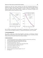
Fig. 6. Comparison of simulated bed pressure drop using different drag models with the
experimental data for a superficial velocity of V
g
= 50 cm/s.


Fig. 7. Comparison of simulated pressure variation versus bed height using Cao-Ahmadi,
Syamlal–O’Brien and Gidaspow drag models with the experimental data for a superficial
velocity of V
g
= 50 cm/s and position of pressure transducers (P1, P2 and P3).
1500
2500
3500
4500
5500
6500
7500
8500
012345
Time (Second)
Pressure difference (Pa)
P1-P3 (Cao-Ahmadi drag)
P1-P3 ( Syamlal-O'Brien drag)
P1-P3 (Gidaspow drag)
Experimental Data
Heat Transfer - Mathematical Modelling, Numerical Methods and Information Technology
352
Fig. 7 compares the simulated pressure variations versus the bed height for different drag
laws with the experimentally measured values. The positions of pressure transducers (P1,

P2 and P3) that were shown in Fig. 4(B) are identified in this Fig. To increase the number of
experimental data for the pressure in the bed, five additional pressure transducers were
installed at the thermocouple locations, and the corresponding pressures for a superficial
velocity of V
g
= 50 cm/s were measured. The air enters into the bed at atmospheric pressure
and decreases roughly linearly from bottom up to a height of about 60 cm due to the
presence of a high concentration of particles. At the bottom of the bed, the solid volume
fraction (bed density) is large; therefore, the rate of pressure drop is larger. Beyond the
height of 60cm (up to 100cm), there are essentially no solid particles, and the pressure is
roughly constant. All three drag models considered show comparable decreasing pressure
trends in the column. The predictions of these models are also in good agreement with the
experimental measurements. Fig.s 6 and 7 indicate that there is no significant difference
between the predicted pressure drops for different drag models for a superficial gas velocity
of V
g
= 50 cm/s.
Figs. 6 and 7 show that there is no significant difference between the predicted pressure
drops and bed expansion ratio for the different drag models used. That is the fluidization
behavior of relatively large Geldart B particles for the bed under study is reasonably well
predicted, and all three drag models are suitable for predicting the hydrodynamics of gas–
solid flows.


Fig. 8. Comparison of experimental and simulated bed pressure drop versus superficial gas
velocity.
Fig. 8 compares the simulated time-averaged bed pressure drops, (P1-P2) and (P1-P3),
against the superficial gas velocity with the experimental data. The Syamlal–O’Brien drag
expression was used in these simulations. The locations of pressure transducers (P1, P2, P3)
were shown in Fig. 4 (B). The simulation and experimental results show good agreement at

velocities above V
mf.
. For V <V
mf,
the solid is not fluidized, and the bed dynamic is
dominated by inter-particle frictional forces, which is not considered by the multi-fluid
models used. Fig. 8 shows that with increasing gas velocity, initially the pressure drops
Study of Hydrodynamics and Heat Transfer in the Fluidized Bed Reactors
353
(P1-P2 and P1-P3) increase, but the rate of increase for (P1-P3) is larger than that for (P1-P2).
For V >V
mf
this Fig. shows that (P1-P3) increases with gas velocity, while (P1-P2) decreases
slightly, stays roughly constant, and increases slightly. This trend is perhaps due to the
expansion of the bed and the decrease in the amount of solids between ports 1 and 2. As the
gas velocity increases further, the wall shear stress increases and the pressure drop begins to
increase. Ports 1 and 3 cover the entire height of the dense bed in the column, and thus (P1-
P3) increases with gas velocity.
As indicated in Fig. 9, the bed overall pressure drop decreased significantly at the beginning
of fluidization and then fluctuated around a near steady-state value after about 3.5 s.
Pressure drop fluctuations are expected as bubbles continuously split and coalesce in a
transient manner in the fluidized bed. The results show with increasing the particles size,
pressure drop increase. Comparison of the model predictions, using the Syamlal–O’Brien
drag functions, and experimental measurements on pressure drop show good agreement for
most operating conditions. These results (for d
s
=0.275 mm) are the same with Tagipour et al.
[8] and Behjat et al. [11] results.

Fig. 9. Comparison of experimental and simulation bed pressure drop (P1-P2) at different
solid particle sizes.
Comparison of experimental and simulated bed pressure drop (Pressure difference between
two positions, P1-P2 and P1-P3) for two different particle sizes, d
s
=0.175 mm and d
s
=0.375
mm, at different superficial gas velocity are shown in Fig. 10. and Fig. 11. Pressure
transducers positions (P1, P2, P3) also were shown in Fig. 4(B). The simulation and
experimental results show better agreement at velocities above U
mf
. The discrepancy for U <
U
mf
may be attributed to the solids not being fluidized, thus being dominated by inter
particle frictional forces, which are not predicted by the multi fluid model for simulating
gas-solid phases.
2500
3500
4500
5500
6500
7500
8500
9500
10500
012345
Time (Second)
Pressure difference (Pa)

ds=0.175 mm (Simulation)
ds=0.275 mm (Simulation)
ds=0.375 mm (Simulation)
ds=0.175 mm (Experimental)
ds=0.275 mm (Experimental)
ds=0.375 mm (Experimental)
Heat Transfer - Mathematical Modelling, Numerical Methods and Information Technology
354

Fig. 10. Comparison of experimental and simulated bed pressure drop at different time


Fig. 11. Comparison of experimental and simulated bed pressure drop at different gas
velocity and particle sizes.
Comparison of experimental and simulated bed pressure drop for two different initial bed
height, H
s
=30, H
s
=40 cm, at different superficial gas velocity are shown in Fig. 11. The
results show with increasing the initial static bed height and gas velocity, pressure drop (P1-
P2 and P1-P3) increase but the rate of increasing for (P1-P3) is larger than (P1-P2).
Comparison of the model predictions and experimental measurements on pressure drop
(for both cases) show good agreement at different gas velocity.
2500
3500
4500
5500
6500
7500

8500
9500
10500
012345
Time (Second)
Pressure difference (Pa)
Hs =20 cm (Simulation)
Hs =30 cm (Simulation)
Hs =40 cm (Simulation)
Hs=20 cm (Experimental)
Hs=30 cm (Experimental)
Hs=40 cm (Experimental)
Study of Hydrodynamics and Heat Transfer in the Fluidized Bed Reactors
355

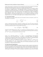
Fig. 12. Comparison of experimental and simulated bed pressure drop at different
superficial gas velocity and static bed height.
These Figs. show that with increasing gas velocity, initially the pressure drops (P1-P2 and
P1-P3) increase, but the rate of increase for (P1-P3) is larger than for (P1-P2). As indicated in
Fig. 12. the bed overall pressure drop decreased significantly at the beginning of fluidization
and then fluctuated around a near steady-state value after about 4 s. Pressure drop
fluctuations are expected as bubbles continuously split and coalesce in a transient manner in
the fluidized bed.
The results show with increasing the initial static bed height, pressure drop increase because
of increasing the amount of particle, interaction between particle-particle and gas-particle.
The results show with increasing the particle size, gas velocity and initial static bed height
pressure drop (P1-P2 and P1-P3) increases. Comparison of the model predictions and
experimental measurements on pressure drop (for both cases) show good agreement at
different gas velocity.
The experimental data for time-averaged bed expansions as a function of superficial

velocities are compared in Fig. 13 with the corresponding values predicted by the models
using the Syamlal–O'Brien, Gidaspow and Cao-Ahmadi drag expressions. This Fig. shows
that the models predict the correct increasing trend of the bed height with the increase of
superficial gas velocity. There are, however, some deviations and the models slightly
underpredict the experimental values. The amount of error for the bed expansion ratio for
the Syamlal-O'Brien, the Gidaspow and Cao-Ahmadi models are, respectively, 6.7%, 8.7%
and 8.8%. This Fig. suggests that the Syamlal–O'Brien drag function gives a somewhat better
prediction when compared with the Gidaspow and Cao-Ahmadi models. In addition, the
Syamlal–O’Brien drag law is able to more accurately predict the minimum fluidization
velocity.
0
1000
2000
3000
4000
5000
6000
7000
8000
9000
10000
0 1020304050607080
Gas velocity (Vg) cm/s
Pressure difference (Pa)
P1-P3(Simulation, Hs=40 cm)
P1-P2 (Simulation, Hs=40 cm)
P1-P2 (Simulation, Hs= 30 cm)
P1-P3 (Simulation, Hs=30 cm)
P1-P2 (Experimental, Hs=30 cm)
P1-P3 (Experimental, Hs=30 cm)

P1-P3 (Experimental, Hs=40 cm)
P1-P2(Experimental, Hs=40 cm)
Heat Transfer - Mathematical Modelling, Numerical Methods and Information Technology
356

Fig. 13. Comparison of experimental and simulated bed expansion ratio.


Fig. 14. Experimental and simulated time-averaged local voidage profiles at z=30 cm, Vg=50
cm/s.
The experimental data for the time-averaged voidage profile at a height of 30 cm is
compared with the simulation results for the three different drag models in Fig. 14 for V
g
=50
cm/s. This Fig. shows the profiles of time-averaged voidages for a time interval of 5 to 10 s.
In this time duration, the majority of the bubbles move roughly in the bed mid-section
toward the bed surface. This Fig. shows that the void fraction profile is roughly uniform in
the core of the bed with a slight decrease near the walls. The fluctuation pattern in the void
fraction profile is perhaps due to the development of the gas bubble flow pattern in the bed.
Similar trends have been observed in the earlier CFD models of fluidized beds [8, 11]. The
gas volume fraction average error between CFD simulations and the experimental data for
the drag models of Gidaspow, Syamlal–O'Brien and Cao-Ahmadi are, respectively, about
0.6
0.9
1.2
1.5
1.8
2.1
2.4
0 0.2 0.4 0.6 0.8 1

Gas Velocity (Vg) m/s
H/H0
Experi mental
Syml al O'Brien drag
Gi daspow drag
Cao-Ahmadi drag
Study of Hydrodynamics and Heat Transfer in the Fluidized Bed Reactors
357
12.7%, 7.6% and 7.2%. This observation is comparable to those of the earlier works [8, 11]. It
can be seen that Cao- Ahmadi drag expression leads to a better prediction compared with
those of Syamlal–O'Brien and Gidaspow drag models for the time averaged voidage.


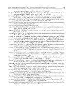
Fig. 15. Comparison of experimental and simulated bed expansion ratio for different solid
particle sizes.
Time-averaged bed expansions as a function of superficial velocities are compared in Fig. 15.
This Fig. shows that the model predicts the correct increasing trend of the bed height with
the increase of superficial gas velocity. All cases demonstrate a consistent increase in bed
expansion with gas velocity and predict the bed expansion reasonably well. There are,
however, some deviations under predict the experimental values. This Fig. shows that with
increasing the particles sizes, bed expansion ratio decreases. On the other hand, for the same
gas velocity, bed expansion ratio is lager for smaller particles.
The experimental data of time-average bed expansion ratio were compared with
corresponding values predicted for various velocities as depicted in Fig. 16. The time-
average bed expansion ratio error between CFD simulation results and the experimental
data for two different initial bed height, H
s
=30, H
s
=40 cm, are 6.7% and 8.7% respectively.

Both cases demonstrate a consistent increase in bed expansion with gas velocity and predict
the bed expansion reasonably well. It can be seen that Syamlal–O'Brien drag function gives a
good prediction in terms of bed expansion and also, Syamlal–O'Brien drag law able to
predict the minimum fluidization conditions correctly.
Simulation results for void fraction profile are show in Fig. 17. In this Fig. symmetry of the
void fraction is observed at three different particle sizes. The slight asymmetry in the void
fraction profile may result form the development of a certain flow pattern in the bed. Similar
asymmetry has been observed in other CFD modeling of fluidized beds. Void fraction
profile for large particle is flatter near the center of the bed. The simulation results of time-
average cross-sectional void fraction at different solid particles diameter is shown in Fig. 18
0.4
0.7
1
1.3
1.6
1.9
2.2
2.5
0 0.2 0.4 0.6 0.8 1
Gas Velocity (Ug) m/s
H/H0
ds=0.175 mm (Simulation)
ds=0.175 mm (Experimental)
ds=0.275 mm (Simulation)
ds=0.275 mm (Experimental)
ds=0.375 mm (Simulation)
ds=0.375 mm (Experimental)
35
fo
r

be
d


Fi
g
st
a


Fi
g
c
m
Heat
T
8
r
U
g
=38 cm/s. T
h
d
hei
g
ht increas
e
g
. 16. Compariso
n

a
tic bed hei
g
ht.
g
. 17. Simulated
v
m
/s, t=5.0s)
1
1.2
1.4
1.6
1.8
2
H/H0
T
ransfer - Mathem
a
h
is Fig. shows w
i
e
and stead
y
stat
e
n
of experimenta
l

v
oid fraction at d
i
01020
Hs=40
c
Hs=40
c
Hs=30
c
Hs= 30
a
tical Modelling, N
u
i
th increasin
g
so
l
e
condition arrive
l
and simulated
b
i
fferent solid par
t
30 40
Gas velocity (
V

c
m (Simulation)
c
m (Experimental)
c
m (Simulation)
cm (Experimental
)
u
merical Methods
a
l
id particles dia
m
rapidl
y
.
b
ed expansion ra
t
t
icles diameter (
a
50 60
V
g) cm/s
)
a
nd Information Te
c

m
eter, void fracti
o

t
io for different i
n

a
t z=20 cm, U
g
=3
8
70 80
c
hnology
o
n and
n
itial
8

Study of Hydrodynamics and Heat Transfer in the Fluidized Bed Reactors
359

Fig. 18. Simulation results of time-average cross-sectional void fraction at different solid
particles diameter (U
g
=38cm/s)

Fig. 19. Simulation results of time-average cross-sectional void fraction at different
superficial gas velocity (H
s
=40 cm)
Fig. 19 shows the simulation results of time-average cross-sectional void fraction, gas
volume fraction, at different superficial gas velocity. This Fig. shows with increasing
superficial gas velocity, void fraction also increase and bed arrive to steady state condition
rapidly. Also in some position the plot is flat, it is means that particle distribution is
uniform. When void fraction increase suddenly in the bed, it is means that the large bubble
product in this position and when decrease, the bubble was collapsed.
0.3
0.4
0.5
0.6
0.7
0.8
0.9
1
0 102030405060708090100
Bed Height (cm)
Void Fraction
ds=0.175 mm
ds=0.275 mm
ds=0.375 mm
0.3
0.4
0.5
0.6
0.7

0.8
0.9
1
0 1020304050607080
Bed Height (cm)
Void fraction
Vg=30 cm/s
Vg=50 cm/s
Vg=70 cm/s
Heat Transfer - Mathematical Modelling, Numerical Methods and Information Technology
360
Fig. 20 shows simulation results for void fraction contour plot, gas volume fraction, for
U
g
= 38 cm/s, d
s
= 0.175 mm. The increase in bed expansion and variation of the fluid-bed
voidage can be observed. At the start of the simulation, waves of voidage are created, which
travel through the bed and subsequently break to form bubbles as the simulation
progresses. Initially, the bed height increased with bubble formation until it leveled off at a
steady-state bed height. The observed axisymmetry gave way to chaotic transient generation
of bubble formation after 1.5 s. The bubbles coalesce as they move upwards producing
bigger bubbles. The bubbles become stretched as a result of bed wall effects and interactions
with other bubbles.



Fig. 20. Simulation void fraction profile of 2D bed (U
g
= 38 cm/s, d

s
= 0.175 mm)
The contour plots of solids fraction shown in Fig. 21 indicate similarities between the
experimental and simulations for three particle sizes and at three different times. The results
show that the bubbles at the bottom of the bed are relatively small. The experiments
indicated small bubbles near the bottom of the bed; the bubbles grow as they rise to the top
surface with coalescence. The elongation of the bubbles is due to wall effects and interaction
with other bubbles. Syamlal–O'Brien drag model provided similar qualitative flow patterns.
The size of the bubbles predicted by the CFD models are in general similar to those
observed experimentally. Any discrepancy could be due to the effect of the gas distributor,
which was not considered in the CFD modeling of fluid bed. In practice, jet penetration and
hydrodynamics near the distributor are significantly affected by the distributor design.
The increase in bed expansion and the greater variation of the fluid-bed voidage can be
observed in Fig. 20 and Fig. 21 for particles with d
s
= 0.175 mm. According to experimental
evidence, this type of solid particle should exhibit a bubbling behavior as soon as the gas
velocity exceeds minimum fluidization conditions.
It is also worth noting that the computed bubbles show regions of voidage distribution at
the bubble edge, as experimentally observed. In Fig. 21 symmetry of the void fraction is
observed at three different particle sizes. The slight asymmetry in the void fraction profile
may result form the development of a certain flow pattern in the bed. Similar asymmetry
has been observed in other CFD modeling of fluidized beds [5, 8]. Void fraction profile for
large particle is flatter near the center of the bed.
Study of Hydrodynamics and Heat Transfer in the Fluidized Bed Reactors
361

Fig. 21. Comparison of experiment and simulated void fraction and bobbles for three
particle sizes and three different times
Fig. 22 shows simulated results for contour plot of solids volume fraction (U

g
=38 cm/s,
d
s
=0.275 mm). Initially, the bed height increased with bubble formation until it leveled off at
a steady-state bed height. The observed axisymmetry gave way to chaotic transient
generation of bubble formation after 3 s. The results show that the bubbles at the bottom of
the bed are relatively small. The bubbles coalesce as they move upwards producing bigger
bubbles. The bubbles become stretched as a result of bed wall effects and interactions with
other bubbles. Syamlal–O'Brien drag model provided similar qualitative flow patterns. The
size of the bubbles predicted by the CFD models are in general similar to those observed
experimentally. Any discrepancy could be due to the effect of the gas distributor, which was
not considered in the CFD modeling of fluid bed. In practice, jet penetration and
hydrodynamics near the distributor are significantly affected by the distributor design.
Heat Transfer - Mathematical Modelling, Numerical Methods and Information Technology
362

Fig. 22. Simulated solids volume fraction profile of 2D bed (Ug=38 cm/s, d
s
=0.275 mm).



Fig. 23. Simulated solid volume fraction contours in the 2D bed (Vg =50 cm/s, drag function:
Syamlal–O’Brien).
Simulation results for solid particle velocity vector fields at different times are shown in Fig.
24. This Fig. shows that initially the particles move vertically; at t= 0.7 s, two bubbles are
formed in the bed that are moved to the upper part of the column. The bubbles collapse
when they reach the top of the column, and solid particle velocity vector directions are
changed as the particles move downward. The upward and downward movement of

particles in the bed leads to strong mixing of the phases, which is the main reason for the
effectiveness of the fluidized bed reactors.
Study of Hydrodynamics and Heat Transfer in the Fluidized Bed Reactors
363

Fig. 24. Simulated solid particle velocity vector fields for different times, Vg=50 cm/s.
Fig. 25 compares the experimental results for bubble formation and bed expansion for
different superficial gas velocities. At low gas velocities (lower than Vg=5.5 cm/s), the
solids rest on the gas distributor, and the column is in the fixed bed regime. When super-
ficial gas velocity reaches the fluidization velocity of 5.5 cm/s, all particles are entrained by
the upward gas flow and the bed is fluidized. At this point, the gas drag force on the
particles counterbalances the weight of the particles. When the gas velocity increases
beyond the minimum fluidization velocity, a homogeneous (or smooth) fluidization regime
forms in the bed. Beyond a gas velocity of 7 cm/s, a bubbling regime starts. With an increase
in velocity beyond the minimum bubbling velocity, instabilities with bubbling and
channeling of gas in the bed are observed. Vg=10 cm/s in Fig. 25 corresponds to this regime.
At high gas velocities, the movement of solids becomes more vigorous. Such a bed condition
is called a bubbling bed or heterogeneous fluidized bed, which corresponds to Vg=20-35
cm/s in Fig. 25. In this regime, gas bubbles generated at the distributor coalesce and grow
as they rise through the bed. With further increase in the gas velocity (Vg=40-50 cm/s in Fig.
25), the intensity of bubble formation and collapse increases sharply. This in turn leads to an
increase in the pressure drop as shown in Fig.s 8-11. At higher superficial gas velocities,
groups of small bubbles break free from the distributor plate and coalesce, giving rise to
small pockets of air. These air pockets travel upward through the particles and burst out at
the free surface of the bed, creating the appearance of a boiling bed. As the gas bubbles rise,
these pockets of gas interact and coalesce, so that the average gas bubble size increases with
distance from the distributor. This bubbling regime for the type of powder studied occurs
only over a narrow range of gas velocity values. These gas bubbles eventually become large
enough to spread across the vessel. When this happens, the bed is said to be in the slugging
regime. Vg=60 cm/s in Fig. 25 corresponds to the slugging regime. With further increase in

the gas superficial velocity, the turbulent motion of solid clusters and gas bubbles of various
size and shape are observed. This bed is then considered to be in a turbulent fluidization
regime, which corresponds to Vg=70-100 cm/s in Fig. 25.
Heat Transfer - Mathematical Modelling, Numerical Methods and Information Technology
364



Fig. 25. Comparison of bubble formation and bed expansion for different superficial gas
velocities.
Comparison of the contour plots of solid fractions in Fig. 24 and the experimental results for
bubble formation and bed expansion in Fig. 25 for Vg=50 cm/s indicates qualitative
similarities of the experimental observations and the simulation results. It should be pointed
out that some discrepancies due to the effect of the gas distributor, which was not
considered in the CFD model, should be expected.
Fig. 26 shows the simulation results of gas volume fraction for different superficial gas
velocities. Initially, the bed height increases with bubble formation, so gas volume fraction
Study of Hydrodynamics and Heat Transfer in the Fluidized Bed Reactors
365
increases and levels off at a steady-state bed height. At the start of the simulation, waves of
voidage are created, which travel through the bed and subsequently break to form bubbles
as the simulation progresses. At the bottom of the column, particle concentration is larger
than at the upper part. Therefore, the maximum gas volume fraction occurs at the top of the
column. Clearly the gas volume fraction of 1 (at the top of the bed) corresponds to the region
where the particles are absent. With increasing superficial gas velocity, Fig. 26 shows that
the gas volume fraction generally increases in the bed up to the height of 50 to 60 cm. The
gas volume fraction then increases sharply to reach to 1 at the top of the bed. Gas volume
fraction approaches the saturation condition of 1 at the bed heights of 63cm, 70cm and 85 cm
for Vg=30 cm/s, 50 cm/s and 80 cm/s, respectively. For higher gas velocities, Fig. 26 shows
that the gas volume fraction is larger at the same height in the bed. This is because the

amount of particles is constant and for higher gas velocity, the bed height is higher. Thus,
the solid volume fraction is lower and gas volume fraction is higher. It should be noted here
that the fluctuations of the curves in this Fig. are a result of bubble formation and collapse.


Fig. 26. Simulation results for gas volume fraction at t=5s (Syamlal–O'Brien drag model).
The influence of inlet gas velocity on the gas temperature is shown in Fig.s 27 and 28. As
noted before, the gas enters the bed with a temperature of 473K, and particles are initially at
300K. Thermocouples are installed along the column as shown in Fig. 2(B). The
thermocouple probes can be moved across the reactor for measuring the temperature at
different radii. At each height, gas temperatures at five radii in the reactor were measured
and averaged. The corresponding gas mean temperatures as function of height are
presented in Fig.s 27 and 28. Fig. 29 shows that the gas temperature deceases with height
because of the heat transfer between the cold particles and hot gas. Near the bottom of
column, solid volume fraction is relatively high; therefore, gas temperature decreases
rapidly and the rate of decrease is higher for the region near the bottom of the column. At
top of the column, there are no particles (gas volume fraction is one) and the wall is
adiabatic; therefore, the gas temperature is roughly constant. Also the results show that with
increasing the gas velocity, as expected the gas temperature decreases. From Fig.s 22-25 it is
seen that with increasing gas velocity, bed expansion height increases.
0.2
0.4
0.6
0.8
1
1.2
0 20406080100
Flui dized Bed Height (cm)
Gas volume fraction
Vg=30 cm/s

Vg=50 cm/s
Vg=80 cm/s
Heat Transfer - Mathematical Modelling, Numerical Methods and Information Technology
366

Fig. 27. Simulation and experimental results for inlet gas velocity effect on gas temperature
in the bed (t=5 min).


Fig. 28.
Comparison of simulation and experimental gas temperature and gas volume
fraction at t=5min for Vg=80 cm/s.
In addition, the gas temperature reaches to the uniform (constant temperature) condition in
the upper region. When gas velocity is 30 cm/s, temperature reaches to its constant value at
a height of about 40 cm; and for Vg=50 cm/s and Vg=80 cm/s, the corresponding gas
temperatures reaching uniform state, respectively, at heights of 50 and 55 cm. Fig. 27 also
shows that the simulation results are in good agreement with the experimental data. The
small differences seen are the result of the slight heat loss from the wall in the experimental
reactor. Fig. 28 shows the gas temperature and the gas volume fraction in the same graph.
452
456
460
464
468
472
476
0 20406080100
Fl uidized Bed Height (cm)
Gas Temperature (K)
Vg=30 cm/s (Simulation)

Vg=50 cm/s(Simulation)
Vg=80 cm/s (Simulation)
Vg=80 cm/s (Experimental)
Vg=30 cm/s (Experimental)
Vg=50 cm/s (Experimental)
454
456
458
460
462
464
466
468
470
472
474
0 102030405060708090100
Fl ui dized Bed hi
g
ht (cm)
Gas Temperature (K)
0.2
0.3
0.4
0.5
0.6
0.7
0.8
0.9
1

1.1
Gas Volume fraction
Gas Temperature (Simulation)
Gas Temperature (Experimental)
Gas volume fraction (Simulation)
St
u
T
h
te
m
pa
co
o

Fi
g
di
f

Fi
g
g
a
Fi
g
di
f
in
c

si
m
u
dy of Hydrodyna
m
h
is Fig. indicates
m
perature is lo
w
rt of the reactor,
o
ler particles is
h
g
. 29. Compariso
n
f
ferent
g
as veloci
t
g
. 30. Simulation
s velocities at z=
5
g
. 29 compares
f
ferent

g
as veloc
c
reases with tim
e
m
ulation results
s
m
ics and Heat Tran
s
that in the re
gi
w
est. Clearl
y
in t
h
the solid volum
h
i
g
her and the te
m
n
of experimenta
l
t
ies (z=50 cm).
results for variat

i
5
0 cm
the time variati
ities with the e
x
e
and the rate of i
s
how that with
i
s
fer in the Fluidized
i
on where the
g
h
e free
g
as flow,
t
e fraction is hi
gh
m
perature decrea
l
and computati
o
i
on of solid parti

c
on of the simu
l
x
perimental data
.
ncrease varies w
i
i
ncreasin
g

g
as v
e
Bed Reactors
g
as volume fract
i
t
here is little he
a
h
er, so the rate o
f
ses faster.
o
nal results for
ga
c

le temperature
w
l
ated
g
as tempe
r
.
This Fig. show
s
i
th somewhat wi
e
locit
y
,
g
as tem
p
i
on is hi
g
hest, t
h
a
t transfer. In the
f
heat transfer w
i

a
s temperatures a

w
ith time at diffe
r
r
ature at z=50
c
s
that
g
as temp
e
th the
g
as veloci
t
p
erature reaches
367
h
e
g
as
lower
i
th the
t
r

ent
c
m for
e
rature
ty
. The
stead
y

Heat Transfer - Mathematical Modelling, Numerical Methods and Information Technology
368
state condition rapidly. For Vg=80 cm/s, gas temperature reaches steady state condition
after about 30 min; but for Vg=50 and 30 cm/s temperature reaches to steady after 40 and
45min, respectively but there are a few difference between simulation and experimental
results.
For different inlet gas velocities, time variations of the mean solid phase temperature at the
height of z=50 cm are shown in Fig. 30. The corresponding variation of the averaged solid
particle temperature with height is shown in Fig. 31. Note that, here, the averaged solid
temperature shown is the mean of the particle temperatures averaged across the section of
the column at a given height. It is seen that the particle temperature increases with time and
with the distance from the bottom of the column. Fig. 30 also shows that at higher gas
velocity, solid temperature more rapidly reaches the steady state condition. For Vg=80cm/s,
solid temperature approaches the steady limit after about 30min; for Vg=50 and 30 cm/s,
the steady state condition is reached, respectively, at about 40 and 45min. In addition,
initially the temperature differences between solid and gas phases are higher; therefore, the
rate of increase of solid temperature is higher. Fig. 31 shows that the rate of change of the
solid temperature near the bottom of the bed is faster, which is due to a larger heat transfer
rate compared to the top of the bed. These Fig.s also indicate that an increase in the gas
velocity causes a higher heat transfer coefficient between gas and solid phases, and results

in an increase in the solid particle temperature.


Fig. 31. Inlet gas velocity effect on the simulated solid particle temperatures in bed (t=5min).
The influence of initial bed height (particle amount) on the gas temperature at t=5s is shown
in Fig. 32 experimentally and computationally. It indicates that with increasing the particle
amount, due to a higher contact surfaces and heat transfer between hot gas and cold solid
phase, gas temperature decreases.
The rate of gas temperature decreasing for H
s
=40 cm is larger than H
s
=20 cm because with
increasing the particle amount, volume of cold solid particles and contact surface with hot
gas increase. The effects of static initial bed height on solid phase temperature are shown in
Fig. 33. It indicates that a decrease in particle amount causes a higher void fraction, gas
volume fraction, and heat transfer coefficient between gas and solid phases (resulting in a
St
u
hi
g
in
g
a
in
c
an
o
p

Fi
g
te
m

Fi
g
(V
In
be
c
u
dy of Hydrodyna
m
g
her contact surf
a
solid particle te
m
s temperature d
e
c
reasin
g
for Hs=
4
d experimental
m
p
eratin

g
conditio
n
g
. 32. Compariso
n
m
perature at t=5
s
g
. 33. Simulation
g
=50 cm/s).
addition, the te
m
c
ause inlet
g
as t
e
Solid Phase temperature (K)
m
ics and Heat Tran
s
a
ce between hot
g
m
perature. So w
i

e
creases (Fi
g
. 32)
4
0cm is lar
g
er th
a
m
easurements o
n
n
s.
n
of simulation a
n
s
(V
g
=50 cm/s).
results of initial
b
m
perature
g
radi
e
e
mperature is th

e
300
300.5
301
301.5
302
302.5
303
303.5
304
010
H
H
H
s
fer in the Fluidized
g
as and cold soli
d
i
th increasin
g
th
e
and solid phas
e
a
n others (Fig. 3
3
n

mean
g
as tem
p
n
d experimental
b
ed hei
g
ht effect
e
nt between sol
i
e
hi
g
hest and sol
i
20 30 40

Bed height
(
H
s=20 c
m
H
s=30 c
m
H
s=40 c

m
Bed Reactors
d
phase) that in t
u
e
initial bed hei
g
e
temperature in
c
3
). Comparison o
f
p
erature show
g
o
results of bed he
i
on solid particle
t
i
d and
g
as phas
e
i
d particles temp
50 60 70

(
cm)
u
rn leads to an i
n
g
ht from 20cm to
c
reases and rate
f
the model pred
od a
g
reement fo

ig
ht effect on
g
as

t
emperature at t
=
e
s is hi
g
her at t
h
erature is lowes
t

80
369
n
crease
40cm,
of this
ictions
r most
=
5s
h
e bed
t
in the
37
be
d
fr
a
of
in
d
be
t
de
co
m

Fi
g

di
f

Fi
g
Si
m
Fi
g
Heat
T
0
d
. The slope of t
e
a
ction that leads
t
the bed. The infl
d
icates that wit
h
t
ween
g
as and
creasin
g
with i
n

m
pared reasona
b
g
. 34. Compariso
n
f
ferent
g
as veloci
t
g
. 35. Simulation
m
ulation results
f
g
. 35. From resul
t
T
ransfer - Mathem
a
e
mperature plot
s
t
o a lar
g
er conta
c

uence of inlet
g
a
s
h
increasin
g
the
solid phases,
ga
n
creasin
g
the
g
a
b
l
y
well with exp
e
n
of experimenta
l
ty
(H
s
=40 cm, t=
5
results for heat t

r
f
or heat transfer
c
t
s of this Fig., he
a
a
tical Modelling, N
u
s
is hi
g
her at the
t
c
t surfaces and h
e
s
velocit
y
on the

g
as velocit
y
,
d
a
s temperature

d
s velocit
y
incre
a
e
rimental data.
l
and computati
o
5
s)
r
ansfer coefficien
c
oefficient at diff
a
t transfer coeffi
c
u
merical Methods
a
t
op of the bed d
u
e
at transfer rate c
g
as temperature
d

ue to hi
g
her h
e
d
ecrease rapidl
y

a
se rapidl
y
. The
o
nal results of
g
a
s
t at different
g
as
erent
g
as velocit
i
c
ient increases fr
o
a
nd Information Te
c

u
e to lar
g
er
g
as
v
ompared to the
b
is showed in Fi
g
e
at transfer coe
f
and also rate
o
modelin
g
pred

s
temperature at

velocities (t=7 s)
.
i
es at t=7s are sh
o
o
m bottom to to

p
c
hnology
v
olume
b
ottom
g
. 34. It
f
ficient
o
f this
ictions
.

o
wn in
p
in the
Study of Hydrodynamics and Heat Transfer in the Fluidized Bed Reactors
371
column because with results of Fig. 35. gas volume fraction increases from bottom to top.
This Fig. also indicates that an increase in the gas velocity causes a higher heat transfer
coefficient between gas and solid phases.
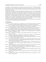
6. Conclusions
In this chapter, unsteady flow and heat transfer in a gas–solid fluidized bed reactor was
investigated. Effect of different parameters for example superficial gas velocity and
temperature, initial static bed height and solid particles diameter on hydrodynamics of a
two-dimensional gas–solid fluidized bed reactor was studied experimentally and

computationally. The Eulerian-Eulerian model with the standard k - ε turbulence model was
used for modeling the fluidized bed reactor. The model includes continuity, momentum
equations, as well as energy equations for both phases and the equations for granular
temperature of the solid particles. A suitable numerical method that employed finite volume
method was applied to discritize the governing equations. In order to validate the model, an
experimental setup was fabricated and a series of tests were performed. The predicted time-
average bed expansion ratio, pressure drop and cross-sectional voidage profiles using Cao-
Ahmadi, Syamlal–O'Brien and Gidaspow drag models were compared with corresponding
values of experimentally measured data. The modeling predictions compared reasonably
well with the experimental bed expansion ratio measurements and qualitative gas–solid
flow patterns. Pressure drops predicted by the simulations were in relatively close
agreement with the experimental measurements for superficial gas velocities higher than the
minimum fluidization velocity. Results show that there is no significant difference for
different drag models, so the results suggest that all three drag models are more suitable for
predicting the hydrodynamics of gas–solid flows. The simulation results suggested that the
Syamlal–O'Brien drag model can more realistically predict the hydrodynamics of gas–solid
flows for the range of parameters used in this study. Moreover, gas and solid phase
temperature distributions in the reactor were computed, considering the hydrodynamics
and heat transfer of the fluidized bed using Syamlal–O'Brien drag expression. Experimental
and numerical results for gas temperature showed that gas temperature decreases as it
moves upwards in the reactor. The effects of inlet gas velocity, solid particles siizes and
initial static bed height on gas and solid phase temperature was also investigated. The
simulation showed that an increase in the gas velocity leads to a decrease in the gas and
increase in the solid particle temperatures. Furthermore, comparison between experimental
and computational simulation showed that the model can predict the hydrodynamic and
heat transfer behavior of a gas-solid fluidized bed reasonably well.
7. Acknowledgments
The authors would like to express their gratitude to the Fluid Mechanics Research Center in
Department of Mechanical Engineering of Amirkabir University, National Petrochemical
company (NPC) and the Petrochemistry Research and Technology Company for providing

financial support for this study.
8. Appendix
In this section drive an algebraic (discretized) equation from a partial differential equation
[39, 40].
Heat Transfer - Mathematical Modelling, Numerical Methods and Information Technology
372
Continuity equation
For this demonstration the transport equation for a scalar  is (m = 0, 1 for solid and gas
phases):























0
(A1)


Fig. A1.
Control volume and node locations in x-direction
With integrating this Equation over a control volume (Fig. A1) and write term by term, from
left to right as follows:
Transient term

























∆
∆
(A2)
where the superscript ‘o’ indicates old (previous) time step values.
Convection term

























































































































(A3)
Combining the equations derived above Discretized Transport Equation is get















+








































+







































=0
(A4)
where the macroscopic densities define as ρ′

α

ρ


Equation (A4) may be rearranged to get the following linear equation for
 , where the
subscript nb represents E, W, N and S [39, 40].





∑







, 


∑


(A5)
The discretized form of continuity equation can be easily by setting  = 1 and a linear
equation of the form (A4), in which the coefficients are defined as follows:



































(A6)
Study of Hydrodynamics and Heat Transfer in the Fluidized Bed Reactors
373


































(A7)



∑




















b=





(A8)
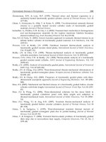
Momentum equation

The discretization of the momentum equations is similar to that of the scalar transport
equation, except that the control volumes are staggered. As explained by Patankar, if the
velocity components and pressure are stored at the same grid locations a checkerboard

pressure field can develop as an acceptable solution. A staggered grid is used for preventing
such unphysical pressure fields. As shown in Fig.A2, in relation to the scalar control volume
centered around the filled circles, the x-momentum control volume is shifted east by half a
cell. Similarly the y-momentum control volume is shifted north by half a cell, control
volume is shifted top by half a cell.
For calculating the momentum convection, velocity components are required at the
locations E, W, N, and S. They are calculated from an arithmetic average of the values at
neighboring locations [39, 40]:











1






(A9)












1






(A10)


Fig. A2. X-momentum equation control volume
A volume fraction value required at the cell center denoted by p is similarly calculated.












1






(A11)


















(A12)
Now the discretized x-momentum equation can be written as











































(A13)
The above equation is similar to the discretized scalar transport equation , except for the last
two terms: The pressure gradient term is determined based on the current value of Pg and is
added to the source term of the linear equation set. The interface transfer term couples all
the equations for the same component.
The definitions for the rest of the terms in Equation (A13) are as follows:








































(A14)