The Behavior of Structures Composed of Composite Materials Part 5 pps

109
3.9 Quasi-Isotropic Composite Panels Subjected to a Uniform Lateral Load
When a composite laminate has a stacking sequence in which it is
referred to as quasi-isotropic. In that case it behaves as an isotropic plate in the
determination of lateral deformations, w
(
x, y ), and stress couples, and
For isotropic plate monocoque plates several textbooks such as Timoshenko and
Woinowsky-Krieger [4] and Vinson [7] have provided expressions for the maximum
deflection, and the maximum stress couple,
M
, a plate attains when subjected to a
constant laterally distributed load such as,
where a is the smaller plate dimension; b
is
the longer plate dimension, E is the
modulus of elasticity of the plate; h is the plate thickness; and
The dimensionless constants and are given in tabular form for various
boundary conditions, and these are repeated herein for completeness in Tables 3.1
through 3.4. Table 3.5 also provides information for the case wherein the plate is
subjected to a hydraulic head. These tables and procedures are well known and well
used.
110
Of course, for the isotropic plate, the flexural stiffness is given by
and the maximum bending stress, which occurs on the top and bottom surfaces of the
plate, is
Also for Tables 3.1 through 3.5, the numerical coefficients correspond to a
Poisson’s ratio of wherein Therefore, for materials with other
Poisson ratios, ,, Equation (3.71) must be changed to
111
With Equations (3.75) and (3.72), the well-used Tables 3.1 through 3.4 for

monocoque plates can be used to analyze quasi-isotropic composite plates as well. It
must be remembered that for these classical theory solutions no transverse-shear
deformation effects are included. Table 3.5 can be used to analyze and design composite
material plates subjected to a hydraulic head.
It is seen that for a monocoque quasi-isotropic plate design,
The plate must not be overstressed, i.e., the maximum stress is determined from the
use of Equation (3.72) to determine the maximum stress couple, M, and the
procedures described earlier to determine the stresses in each lamina. The
determined maximum stress cannot exceed some allowable stress, defined by
the material’s ultimate stress or yield stress divided by a factor of safety on ultimate
stress or yield stress, whichever is smaller. This requires a certain value of plate
thickness, h.
The monocoque plate must not be over deflected determined by Equation (3.75).
This is sometimes specified, but in other cases the plate deflection cannot exceed
the plate thickness or some fraction thereof. If the maximum plate deflection
reaches a value of the plate thickness, h, the equations discussed herein become
inapplicable because the plate behavior becomes increasingly nonlinear which
requires that other equations be used. Again, to prevent over deflection, a plate
thickness, h, is required as determined by Equation (3.75).
(1)
(2)
Therefore, in monocoque plate design, the plate thickness, h, is determined either from a
strength or stiffness requirement, whichever requires the larger thickness.
3.10 A Static Analysis of Composite Material Panels Including Transverse Shearr
Deformation Effects
The previous derivations have involved "classical" plate theory, i.e., they have
neglected transverse shear deformation effects. Because in many composite material
laminated plate constructions, transverse-shear deformation effects are important, a more
refined theory will now be developed. However, because of its simplicity, and the
number of solutions available, classical theory is still useful for preliminary design and

analysis to size the structure required in minimum time and effort.
In the simpler classical theory, the neglect of transverse shear deformation effects
means that To include transverse shear deformation effects, one uses
112
Now substituting the admissible forms of the displacement for a plate or panel,
Equation (2.49) into Equations (3.76) and (3.77), shows that
No longer are the rotations and explicit functions of the derivatives of the
lateral deflection w, as shown by Equation (3.23) for classical plate theory. The result is
that for this refined theory there are five geometric unknowns, and
instead of just the first three in classical theory.
Now one needs to look again at the equilibrium equations, the constitutive
equations (stress-strain relations), the strain-displacement relations and the compatibility
equations. For the plate, the equilibrium equations are given by Equations (3.9) through
(3.15), because they do not change from classical theory. The constitutive equations for a
composite material laminated plate and sandwich panel are given by Equations (2.58)
through (2.66). The new cogent strain-displacement (kinematic) relations are given
above in Equation (3.78) and (3.79). Because the resulting governing equations are in
terms of displacements and rotations, any single valued, continuous solution will by
definition satisfy the compatibility equations.
As an example consider a plate that is mid-plane symmetric and has no
coupling terms the constitutive equations for this orthotropic
plate can be written as follows, where is a transverse shear coefficient to be discussed
later.
113
Because the plate is mid-plane symmetric there is no bending-stretching coupling,
hence the in-plane loads and deflections are uncoupled (separate)
from the lateral loads, deflections and rotations. Hence, for the lateral distributed static
loading, p
(
x, y

)
, Equations (3.16) through (3.18) and Equations (3.83) through (3.87) are
utilized: 8 equations and 8 unknowns.
Substituting Equations (3.83) through (3.87) into Equations (3.16) through (3.18)
and using Equation (2.66) results in the following set of governing differential equations
for a laminated composite plate subjected to a lateral load, with
and no applied surface shear stresses (for simplicity)
The inclusion of transverse shear deformation effects results in three coupled
partial differential equations with three unknowns, and w, contrasted to having one
partial differential equation with one unknown, w, in classical plate (panel) theory; see
Equation (3.29). Incidentally if one specified that and substituting
that into Equations (3.88) through (3.90) reduces the three equations to Equation (3.29),
the classical theory equation. The symbol with no subscript in (3.88) through (3.90) is
a transverse shear deformation shape factor which varies from 1 to 2 depending upon the
geometry.
The classical plate theory governing partial differential equation is fourth order in
both x and y, and therefore requires two and only two boundary conditions on each of the
four edges, as discussed in Section 3.4. This refined theory, including transverse shear
114
deformation, is really sixth order in both x and y, and therefore requires three boundary
conditions on each edge as discussed in Section 3.11 below.
If the laminated plate is orthotropic but not mid-plane symmetric, i.e.,
the governing equations are more complicated than Equations (3.88) through (3.90) and
are given by Whitney [8], Vinson [9] and are discussed briefly in Section 3.23 below.
3.11 Boundary Conditions for a Plate Using the Refined Plate Theory Which
Includes Transverse Shear Deformation
3.11.1. SIMPLY-SUPPORTED EDGE
Again Equation (3.30) holds, but now a third boundary condition is required for
the plate bending because it can be shown that Equations (3.88) through (3.90) are sixth
order in w with respect to x and y. In addition, since the in-plane and lateral behavior are

coupled, a fourth boundary condition enters the picture as well. This has resulted in the
use of two different simply supported boundary conditions, both of which are
mathematically admissible as natural boundary conditions (to be discussed later) and are
practical structural boundary conditions. By convention the simply supported boundary
conditions are given as follows:
where is the mid-surface displacement in the x-direction and is the mid-surface
displacement in the
y
-direction.
Whether one uses S1 or S2 boundary conditions is determined by the physical
aspects of the plate problem being studied.
3.11.2. CLAMPED EDGE
Similarly, for a clamped edge the lateral deflection w and the rotation or
(for an x = constant edge or a y = constant edge, respectively) are zero (note: the slope is
not zero) and the other boundary conditions are analogous to Equation (3.31).
115
3.11.3. FREE EDGE
The free edge requires three boundary conditions on each edge; therefore, it is no
longer necessary to resort to the difficulties of the Kirchhoff boundary conditions for the
bending of the plate needed for classical plates. The boundary conditions for the bending
of the plate are simply:
where n and t are directions normal to and tangential with the edge. Again, the in-plane
boundary conditions for the free edge are
3.11.4. OTHER BOUNDARY CONDITIONS
In addition to the above boundary conditions, which are widely used to
approximate the actual structural boundary conditions, sometimes it is desirable to
consider an edge whose lateral deflection is restrained, whose rotation is restrained or
both. The means by which to describe these boundary conditions is given for example in
[7, pp. 20-21].
3.12 Composite Plates on An Elastic Foundation

Consider a composite material plate that is supported on an elastic foundation. In
most cases an elastic foundation is modeled as an elastic medium with a constant
foundation modulus, i.e., a spring constant per unit planform area, of
k
in units such as
Therefore, the elastic foundation acts on the plate as a force in the negative
direction proportional to the local lateral deflection w
(
x,y
)
. The force per unit area is -kw,
because when w is positive the foundation modulus is acting in a negative direction, and
vice versa. In order to incorporate the effect of the elastic foundation modeled as above
one simply adds another force to the p
(
x,y
)
load term. The results are, that for classical
theory, Equation (3.29) is modified to (3.94), and for the refined theory, Equation (3.90)
is modified to Equation (3.95):
116
3.13 Solutions for Plates of Composite Materials Including Transverse-Shear
Deformation Effects, Simply Supported on All Four Edges
Some solutions are now presented for the equations in Section 3.10 and 3.11,
using the governing differential equations (3.88) through (3.90). In the following with
no subscript is a transverse shear factor, often give as or 5/6.
Dobyns [10] has employed the Navier approach to solving these equations for a
composite plate simply supported on all four edges subjected to a lateral load, using the
following functions:
It is seen that Equations (3.96) through (3.98) satisfy the simply supported boundary

conditions on all edges given in Equation (3.91).
Substituting these functions into the governing differential equations (3.88)
through (3.90) results in the following:
if and is the lateral load coefficient of (3.99) above, then
the operators are given by the following:
117
Solving Equation (3.100), one obtains
where det is the determinant of the [
L
] matrix in Equation (3.100).
Having solved the problem to obtain and w, the curvatures
and may be obtained. These then can be
substituted back into Equations (3.20) through (3.22) to obtain the stress couples
and to determine the location where they are maximum, to help in determining
where the stresses are maximum.
For a laminated composite plate, to find the bending stresses in each lamina one
must use the above equations to find the values for and in Equation (3.23).
Finally, for each lamina the bending stresses can be found using:
The stresses in each lamina in each direction must be compared to the strength of
the lamina material in that direction. Keep in mind that quite often the failure occurs in
the weaker direction in a composite material.
Looking at the load p
(
x,y
)
in Equation (3.99), if the lateral load p
(
x,y
)
is

distributed over the entire lateral surface, then the Euler coefficient, is found to be
118
If that load is uniform then,
For a concentrated load located at and
where P is the total load.
For loads over a rectangular area of side lengths
u
and v whose center is at and
as shown in Figure 3.8, is given as follows:
119
where P is the total load. Note that when n/b = 1/v, m/a = 1/u, then Of course,
any other lateral load can be characterized by the use of Equation (3.105).
3.14 Dynamic Effects on Panels of Composite Materials
Seldom in real life is a structure subjected only to static loads. More often
products and structures are subjected to vehicular, impact, crash, earthquake, handling, or
fabricating dynamic loads. In the linear-elastic range, dynamic effects can be divided
into two categories: natural vibrations and forced vibrations, and the latter can be further
subdivided into one-time events (an impact) or recurring loads (such as cyclic loading).
These will be discussed in turn.
Physically every elastic continuous body has an infinity of natural frequencies,
only a few of which are of practical significance. When a structure is excited cyclically
at a natural frequency, it takes little input energy for the amplitude to grow until one of
four things happens:
The amplitude of vibration grows until the ultimate strength of a brittle material is
exceeded and the structure fails.
Portions of the structure exceed the yield strength, plastically deform and the
behavior changes drastically.
The amplitude grows until nonlinear effects become significant, and there is no
natural frequency.
Due to damping or other mechanism the amplitude is limited, but as the natural

vibration continues, fatigue failures may occur.
(1)
(2)
(3)
(4)
Physically, when a structure is undergoing a natural vibration the sum of the
potential energy and kinetic energy remains constant if no damping is present. This can
be termed a conservative system. However, the energy is compartmentalized, i.e., if a
structure is truly vibrating in one mode of natural vibration it will not change and
commence vibration in some other mode of natural vibration at some other natural
frequency. In a complex structure if two components have vibrational natural
frequencies that are identical, then when one component is excited, the other component
will also be excited. It is for this very reason that duplicative natural frequencies are to
be avoided. Also in complex structures of course the structural natural frequencies can
be coupled involving all components.
Mathematically, natural vibration problems are called eigenvalue problems. They
are represented by homogeneous equations, for which nontrivial solutions only occur at
certain characteristic
(
eigen
,
in German) values of a parameter, from which the natural
frequencies are determined. In a natural vibration the displacement field comprises a
120
normal mode. At any two different natural frequencies the corresponding normal modes
are orthogonal to each other hence the compartmentalization of the energy). The normal
modes comprise the solutions to the homogeneous governing differential equations,
which are now zero only at the eigenvalues for those equations and boundary conditions.
If there is a forcing function, then the particular solution for the specific forcing
function (which can be cyclical or a one time dynamic impact load) is added onto the

homogeneous solution, which involves the natural frequencies and mode shapes.
Physically, any dynamic load excites each and every one of the normal modes and
corresponding natural frequencies. Usually, only a relatively few are large enough to be
of concern. The largest amplitude of response will be in those mode shapes whose
natural frequency is closest to the oscillatory component of the forcing functions.
When there are no natural frequencies close to the oscillatory portion of the
dynamic load, then the structure will respond in deflection and stresses corresponding
only to the magnitude and spatial distribution of the load. Such a condition results in
solving the worst-case static problem in which the biggest load at some time, t, is applied.
This is termed a quasistatic case. However, if the dynamic load oscillatory component is
close to one of more natural frequencies, then the structural response can be much larger
than the value obtained from a quasistatic calculation, and that increase can be
represented by a dynamic load factor.
In what follows natural frequencies are treated first, then forced linear vibrations
and finally nonlinear large-amplitude vibrations are discussed.
3.15 Natural Flexural Vibrations of Rectangular Plates: Classical Theory
Consider a rectangular composite material plate that is mid-plane symmetric such
that If this plate is isotropic, i.e., then the governing
differential equation is given by Equation (3.29) for the classical theory, i.e., no
transverse-shear deformation, and repeated here as
For dynamic loads, using d’Alembert’s Principle, the equation is written as
where the last term is the mass per unit planform area times the acceleration. For natural
vibrations the load (the forcing function) can be ignored and the resulting homogeneous
equation is
121
This equation yields all of the natural frequencies for plates with any boundary
conditions. For the easiest case, consider the composite material plate to be simply
supported on all four edges. In that case, one may guess the following form for the
deflection function because it satisfies all boundary conditions:
where is the natural circular frequency in radians per unit time. Note that instead of

one may use either or where and the results
will be the same.
Substituting Equation (3.112) into Equation (3.111) one sees that the nontrivial
solution exists only when
In the above m and n are integers only. In this case, the lowest natural frequency occurs
when m = n= 1, and this lowest frequency is always termed the fundamental natural
frequency. To obtain the natural frequency in terms of cycles per second (Hz)
Equation (3.113) is more accurate at low values of m and n, but as these integers
increase, i.e., higher mode shapes, the calculated values increasingly exceed measured
values. This is because transverse shear deformation effects increase with increased
values of m and n, i.e., with the increased ratio of plate thickness to the wavelength of the
m-n
th
mode of vibration. One major reference on the free vibrations of rectangular
isotropic plates is Leissa [11].
If the composite plate is specially orthotropic and mid-plane symmetric, then for
the natural vibration problem the governing differential equation is written as in Equation
(3.29),
122
Again
,
if all four edges are simply supported then the mode shapes are give by Equation
(3.112) with the result that the natural circular frequency in radians per second is given
by
Again, the natural frequency in Hz is given by Equation (3.114).
Keep in mind that for Equation (3.116) and other equations for the frequencies for
natural vibrations to accurately describe the motion, the maximum deflection must be a
fraction of the plate thickness since the theory is linear. Above that level of motion,
nonlinear effects become increasingly significant.
3.16 Natural Flexural Vibrations of Composite Material Plates Including

Transverse-Shear Deformation Effects
The governing partial differential equations for a composite plate or panel that is
specially orthotropic and mid-plane symmetric subjected to a lateral static load p
(
x,y
)
are
given in Equations (3.88) through (3.90). If one now wishes to find the natural
frequencies of this composite plate, that has mid-surface symmetry no other
couplings but includes transverse shear deformation,
then one sets p
(
x,y
)
= 0 in Equation (3.90), but adds to the
right-hand side. In addition, because and are both dependent variables that are
independent of w, there will be an oscillatory motion of the lineal element across the plate
thickness about the mid-surface of the plate. This results in the last term on the left-hand
side of Equations (3.88) and (3.90) becoming and
respectively, as shown below:
123
where is given by
where is the mass density of the kth lamina, and here
I
is
In Equations (3.117) through (3.119) the ’s are transverse-shear deformation
parameters, as discussed earlier.
Similar to the Navier procedure used in previous analyses and following Dobyns
[10] for the simply supported plate let
Substituting these into the dynamic governing equations above results in a set of

homogeneous equations that can be solved for the natural frequencies of vibration
where the unprimed
L
quantities were defined below Equation (3.100) and
124
Three eigenvalues (natural frequencies) result from solving Equation (3.125) for
each value of m and n. However, two of the frequencies are significantly higher than the
other because they are associated with the rotatory inertia terms, which are the last terms
on the left-hand sides of Equations (3.117) and (3.118) and are very seldom important in
structural responses. If they are neglected then and above, and the
square of the remaining natural frequency can be easily found to be
where, here, Also,
If transverse-shear deformation effects were neglected, Equation (3.126) would reduce to
the following result for the case of a mid-plane symmetric, specially orthotropic
composite laminated classical plate, simply supported on all four edges.
where is the mass density per unit planform area. If this plate is isotropic (3.127)
becomes identical to (3.113).
3.17 Forced-Vibration Response of a Composite Material Plate Subjected to a
Dynamic Lateral Load
Dobyns [10] then goes on to develop the solutions for the simply supported
laminated composite plate subjected to a dynamic lateral load p
(
x,y,t
)
, neglecting the
rotatory inertia terms discussed above, utilizing a convolution integral P
(
t
)
as seen below

in (3.131). Incidentally, the convolution integral is also known as the superposition
integral and the Duhamel integral.
His solutions are also applicable to specially orthotropic composite material plates
using the proper stiffness matrix quantities. The solutions to Equations (3.117) through
125
(3.119), modified to include a dynamic distributed lateral load p
(
x,y,t
)
and neglecting the
rotatory inertia terms are given by
where
and is the coefficient of the lateral-load function expanded in series form [see
Equation (3.105)].
So for a given lateral distributed load p
(
x,y,t
)
, if a solution of the form given by
Equations (3.128) through (3.130) is applicable, then the curvatures and for
the plate can be found from Equation (3.23), and the stresses in each lamina are found
from Equation (3.104). The function P
(
t
)
has been solved analytically for several
representative forcing functions shown in Figure 3.9.
For the sine pulse, the forcing function F
(
t

)
and the convolution integral P
(
t
)
are
126
For the stepped pulse the forcing function F
(
t
)
and the convolution integral P
(
t
)
are given
For a triangular pulse:
127
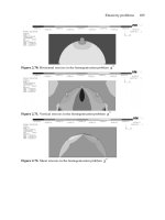
The stepped triangular pulse of Figure 3.9 simulates a nuclear-blast loading [10]
where the pressure pulse consists of a long-duration phase of several seconds due to the
overpressure and a short-duration phase of a few milliseconds due to the shock wave
reflection. The short-duration phase has twice the pressure of the long-duration phase.
128
129
Lastly, the exponential pulse of Figure 3.9 may be used to simulate a high
explosive (non-nuclear) blast loading when the decay parameter is empirically
determined to fit the pressure pulse of the actual blast. The equations are
It should be noted that although the forcing-function equations given above are used
herein to investigate the dynamic response of a composite material plate, these equations
are useful for many other purposes.

Dobyns [10] concludes that the equations presented in this section allow one to
analyze a composite material panel subjected to dynamic loads with only a little more
effort than is required for the same panel subjected to static loads. He stated that one
does not have to rely upon approximate design curves or arbitrary dynamic-magnification
load factors.
With the information presented to this point, the necessary equations for the study
of a composite plate without various couplings, but that include transverse-shear
deformation, have been developed. The plate may be subjected to various static loads
and a variety of dynamic loads. These loads and solutions can be used singly-or
superimposed-to describe a complex dynamic input. (Those same load functions can be
used for beams, shells and many other structural configurations.) With the solutions for
and w, maximum deflections and stresses can be determined for
deflection stiffness-critical and strength-critical structures.
Vibration Damping
Damping of composite structures is clearly beyond the scope of this basic
textbook. However, it would be a mistake not to mention that composite structures
incorporate significant damping through the intrinsic properties of composite materials
compared to metallic structures.
For the study of vibration damping, the text by Nashif, Jones, and Henderson [12]
is excellent. Also, the text by Inman [13] concerning vibrations, vibrations damping,
control, measurement and stability provides much needed information useful to the study
of composite material structural vibrations.
130
3.18 Buckling of a Rectangular Composite Material Plate – Classical Theory
In addition to looking at maximum deflections, maximum stresses and natural
frequencies when analyzing a structure, one must investigate under what loading
conditions an instability can occur, which is also generically referred to as buckling.
For a mid-plane symmetric plate there are five equations associated with the in-
plane loads and and the in-plane displacements they cause, and
These equations are give by (3.9), (3.10) and (2.66), for the case of mid-plane symmetry

it is seen that
Likewise the six governing equations involving and w, are
given by Equations (3.12), (3.14), (3.15), (3.24), (3.25) and (3.26). At any rate there is
no coupling between in-plane and lateral action for the plate with mid-plane symmetry.
Yet is it well known and often observed that in-plane loads through buckling do cause
lateral deflections, which are usually disastrous.
The answer to the paradox is the following: Through this Chapter up to this point
we have used a linear elasticity theory, and the physical event of buckling is a non-linear
problem. Because buckling is a non-linear effect, the in-plane strains are given by the
following, where it is seen that the next (non-linear) term in the McLauren series has
been included:
The results of including the terms to predict the advent or inception of buckling
for the plate are given in the following equations, which is Equation (3.29) for a specially
orthotropic plate; modified to include buckling effects:
131
It is clearly seen that there is a coupling between the in-plane loads and the lateral
deflection.
The buckling loads like the natural frequencies are independent of the lateral
loads, which will be disregarded in what follows. However, in actual structural analysis,
the effect of lateral loads, along with the in-plane loads could cause overstressing and
failure before the buckling load is reached. However, the buckling load is independent of
the lateral load, as are the natural frequencies. Incidentally, common sense dictates that if
one is designing a structure to withstand compressive loads, with the possibility of
buckling being the failure mode, one had better design the structure to be mid-plane
symmetric, so that otherwise the bending-stretching coupling could cause
overstressing before the buckling load is reached.
Looking now at Equation (3.146) for the buckling of the composite plate under an
axial load per unit width only, and ignoring p
(
x,y

)
Equation (3.146) becomes:
Again assuming the buckling mode for a laminated composite material plate to be
that of an isotropic plate with the same boundary conditions, then for the case of the plate
simply supported on all four edges one assumes the Navier solution:
Substituting Equation (3.148) into Equation (3.147) it is seen that for the critical
load
where again several things are clear: Equation (3.147) is a homogeneous equation, one
cannot determine the value of and only the lowest value of is of any
importance usually. However, it is not clear which value of m and n result in the lowest
critical buckling load. All values of n appear in the numerator, so n = 1 is the necessary
132
value for this case of all four edges simply supported. But m appears several places, and
depending upon the value of the flexural stiffness and and the length to width
ratio of the plate,
a/b
, it is not clear which value of
m
will provide the lowest value of
However, for a given plate it is easily determined computationally.
Thus, it is seen that the eigenvalue problems differ from the considerations in
previous sections because either event, natural vibration or buckling, occurs at only
certain values. Hence, the natural frequencies and the buckling load are the eigenvalues;
the vibrational mode and the buckling mode are the eigenfunctions.
In analyzing any structure one therefore should determine four things: the
maximum deflection, the maximum stresses, the natural frequencies (if there is any
dynamic loading to the structure – or nearby to the structure) and the buckling loads (if
there are any compressive loads or in-plane shear loads).
What about the natural vibrations and buckling loads of composite material plates
with boundary conditions other than simply supported? It is seen that for the cases

treated in this section that double sine series were used because those are the vibrational
modes and buckling modes of plates simply supported on all edges.
All combinations of beam vibrational mode shapes are applicable for the study of
plates with various boundary conditions. These have been developed by Warburton [14],
and all derivatives and integrals of those functions catalogued conveniently by Young
an
d
Felgar [15, 16] for easy use.
Expressions for buckling and vibrational modes for other boundary conditions are
available in many texts. They can be used instead of Equation (3.148) for the buckling
mode.
It must again be stated that in buckling loads calculated in this section do not
include transverse shear effects, and are therefore only approximate – but they are useful
for preliminary design, because of their relative simplicity. If the transverse shear
deformation were included, see the next section, the buckling loads would be lower than
those calculated in this section – so the buckling loads calculated, neglecting transverse
shear deformation, are not conservative.
3.19 Buckling of a Composite Material Plate Including Transverse Shear
Deformation Effects.
Consider the same composite material plate discussed in Section 3.18. However,
herein the effects of transverse shear deformation will be included. The constitutive
equations are given in (2.66), where the curvatures are defined by (3.23).
For the buckling of the plate due to in-plane loads, the equilibrium equations for a
buckled plate are [17]:
133
The five equilibrium equations can be written in terms of the five unknowns, the
three displacements, u, v and w, and the two rotations, and Solving the five
coupled partial differential equations with the proper boundary conditions provide the
solution. However, only a few cases have been solved analytically. Moh and Hwu [17]
have given an analytical solution for the composite plate with a cross-ply symmetric

laminate.
Substituting the constitutive equations and the strain displacement relations into
the equilibrium equations provide the following results:
In these equations the and are treated as constants that are known
and remain unchanged during bending. Using the usual assumptions for the deflections
and rotations. Consider the plate to be simply supported on all four edges and subjected
to a biaxial compressive load per unit edge distance such that