Thermal Analysis - Fundamentals and Applications to Polymer Science Part 9 ppsx

Document
Page 112
where W
f
, W
fb
and W
nf
are the freezing, the freezing-bound and the nonfreezing water contents,
respectively. Determination of the exact proportions of these water species in a hydrated polymer is an
important step in understanding the physicochemical processes which govern the behaviour of the
system.
5.12.1 Experimental Procedure
DSC is commonly used to determine the proportions of the various water fractions present in hydrated
polymers. Sample vessels which can be sealed hermetically are required. If aluminium sample vessels
are to be used they should first be placed in an autoclave with a small amount of pure water at 373 K for
3-5 h to eliminate the formation of aluminium hydroxide on the inner surfaces of the sample vessel
during the measuring cycle. Almost all polymers contain a small amount of water which is absorbed
during synthesis, processing or storage. When closely associated with the polymer matrix this water can
remain in the matrix even after heating the polymer to 373 K under reduced pressure. It is important to
establish the concentration of this water species so that the total amount of water present in the sample
after hydration is precisely known. To determine this intrinsic water content the sample should be
weighed as accurately as possible, noting that the sample will absorb water from the atmosphere during
weighing. A microbalance with sensitivity > 0.001 mg is necessary. The sample vessel is pierced,
quickly placed in the DSC at room temperature and heated at 10 K/min. An endothermic deviation in
the sample baseline due to the vaporization of water is observed. The heat of vaporization of water is
high (2257 J/g) and the presence of very small amounts of water can be detected by this procedure. The
sample is heated until no deviation in the sample baseline is observed. The dried sample is then quickly
reweighed and the intrinsic water content determined.
The following procedure is recommended to obtain a uniformly hydrated sample. A precisely known
amount of sample is placed in a sample vessel and an excess amount of distilled, deionized water is

added to the sample using a microsyringe. While monitoring the total mass of the sample vessel and
hydrated polymer, the excess water is allowed to evaporate until the desired water concentration is
achieved. The sample vessel is then hermetically sealed and allowed to equilibrate for 1-7 days. The
storage temperature should be greater than the glass transition temperature of the dry polymer and is
normally in the range 280 -365 K. Natural polymers are prone to acid hydrolysis, resulting in a
reduction of molecular mass, and equilibration of hydrated natural polymers should be carried out at
temperatures ≤ 285 K. The equilibration period is longest for hydrophobic polymers.
The equilibrated sample is placed in the DSC at the storage temperature and cooled at 5 10 K/min to
150 K. The sample is held at 150 K for 15 min and

file:///Q|/t_/t_112.htm2/13/2006 12:58:14 PM
Document
Page 113
heated back to the storage temperature at the same rate. This procedure is repeated three times, the
heating and cooling thermograms being recorded each time. The temperature and number of
crystallization exotherms observed depend on the nature of the polymer and the water concentration.
From the cooling cycle data the proportion of freezing water, W
f
, is calculated by dividing the total area
of the freezing water peak (peak I in Figure 5.27) by the heat of crystallization of bulk water. The
reported value should be the average of the estimates from the three thermal cycles. The heat of
crystallization is not constant for all water species and therefore W
fb
cannot be determined in the same
way. Instead, the total area of the freezing-bound water peak (peak II in Figure 5.27) per gram of dry
polymer should be plotted as a function of water content. The intercept of the linear plot is the amount
of non-freezing water in the hydrated polymer, W
nf
, and the slope is the enthalpy of crystallization of
the freezing-bound water which can be used to calculate W

fb
.
It is not recommended to use the heating cycle data to measure the bound water content as the area of
the endothermic peak does not represent the enthalpy change associated with the transition from ice to
water, but rather the change in enthalpy associated with the transformation from water in a crystalline
state to a homogeneous mixture of water and polymer. The difference is the heat of mixing of water
with the polymer, which is very difficult to estimate. In addition, owing to the complex interplay
between the ice structures present, the non-freezable water fractions and the mobile elements of the
polymer matrix, clear resolution of the different water species during heating is often impossible.
In some cases it is possible to measure the bound water content of a hydrated polymer using TG. The
loss of freezable water occurs from room temperature onwards and a relatively large amount of water
evaporates during handling. These losses, coupled with the losses which occur during the preliminary
heating cycle in the isothermal mode, render estimates of the total water content by TG less reliable
than those from DSC. The bound water fractions are less prone to evaporation during handling and can
be determined from the TG curve. With the DTG curve it is sometimes possible to resolve the peaks
due to the non-freezing and freezing-bound water and to estimate W
nf
and W
fb
.
5.13 Phase Diagram
A phase diagram is a graphical representation of the relationship between a given set of experimental
parameters and the phase changes occurring in a material. Sample volume, transition temperature and
enthalpy, pressure and composition of the material are commonly used parameters in phase diagrams.
Transition temperatures measured by TA are not equilibrium values and vary with the experimental
conditions, particularly the scanning rate. Therefore,

file:///Q|/t_/t_113.htm2/13/2006 12:58:15 PM
Document
Page 114

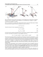
Figure 5.28.
(A) DSC heating curves for water-xanthan gum systems at
various water concentrations: (I) 0.54; (II) 0.57; (III) 0.70; (IV) 0.84; (V)
1.06; (VI) 1.40 g/g. (B) Phase diagram compiled from DSC heating
curves. T
g
, glass transition; T
cc
, cold crystallization; T
m

melting; T*, transition from mesophase to liquid state
when presenting a phase diagram compiled from TA data the experimental conditions must be
described in detail.
Xanthan gum is an anionic polysaccharide secreted by certain bacteria which in the dry state does not
exhibit a first-order phase transition. In the presence of a small amount of water a glass transition, cold
crystallization, melting and a liquid crystal transition are observed. Figure 5.28A presents DSC heating
curves of water-xanthan gum systems with various water contents. A 3 mg sample was hermetically
sealed in an aluminium sample vessel, cooled from 320 to 150 K at 10 K/min and subsequently heated
at 10 K/min. With reference to Section 5.1, the transition temperatures are defined as follows: glass
transition temperature T
ig
and melting and crystallization temperatures T
pm
and T
pc
, respectively. The
corresponding phase diagram, showing the transition temperatures as a function of the water content
(W
c

) for the water-xanthan gum system, is presented in Figure 5.28B. The melting temperature
increases with W
c
levelling off at W
c
= 1.4 g/g. The glass transition temperature decreases in the W
c

range where freezable water (Section 5.12) is no longer present. The liquid crystal transition is observed
between W
c
= 0.45 and 1.0 g/g in the temperature range 260 300 K. The liquid crystalline nature of
water-xanthan gum systems can also be observed under the same conditions by thermomicroscopy
(Section 6.4).

file:///Q|/t_/t_114.htm2/13/2006 12:58:16 PM
Document
Page 115
5.14 Gel-Sol Transition
Polymer chains can form infinite networks by either physical or chemical association. Reversible
networks in the presence of a solvent form reversible gels. The cross-links between individual chains in
a reversible gel are localized, but not permanent, and the interacting groups dissociate and reassociate
according to the conditions of thermodynamic equilibrium. The gel structure present at low
temperatures is transformed on heating and a liquid state is observed. This process, which can be
reversed on cooling, is called the gel-sol transition and can be monitored by HS-DSC. The HS-DSC
curve of the gel-sol transition is often very broad and structured on both heating and cooling. Hysteresis
is generally observed between the heating and cooling cycles. For many gels there is no strict gel point,
rather the gel-sol transition represents a progressive transformation from an elastic state (gel) to a
viscous state (sol). The gel-sol transition is influenced by the molecular mass and polydispersity of the
polymer and also by the nature, concentration, ionic content and pH of the solvent. The presence of

small amounts of impurities can also affect the transition characteristics.
When measuring the enthalpy of transition by HS-DSC, it is important to establish the most appropriate
extrapolated sample baseline. It is generally assumed that the sample baselines observed before and
after the transition can be expressed as linear functions of temperature, and can be extrapolated into the
transition region. For a system which is strictly two-state (A
B). the apparent specific heats are given
by
where W, X, Y and Z and constants and T is the temperature. The extrapolated sample baseline in the
region of the transition is a curve which changes from one apparent specific heat to the other as a
function of the degree of conversion and is given by
where α is the degree of conversion and the constants are determined graphically from the HS-DSC
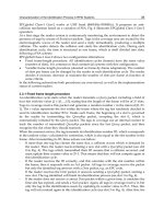
curve. Figure 5.29 shows an extrapolated sample baseline calculated using this method. The enthalpy of
transition can then be estimated using
where
T
1/2
and ∆H
1/2
are the temperature of half-conversion and the enthalpy of transition at half-conversion,
respectively.

file:///Q|/t_/t_115.htm2/13/2006 12:58:17 PM
Document
Page 116
Figure 5.29.
Calculated extrapolated sample
baseline for the HS-DSC heating
curve, using equation 5.50
The ideal behaviour assumed in calculating the enthalpy of transition is rarely observed in gel systems.
Neither the gel nor the sol state are equilibrium states and therefore d(

∆
H)/dT cannot be directly
correlated with ∆C
p
for the transition. The sol state is not an isotropic liquid state, particularly in the
case of DNA and polysaccharides, as high-order structures can be formed in the sol state, greatly
affecting the gel structure subsequently formed on cooling. In the case where the polymer behaves as a
linear polyelectrolyte, there is a contribution to the enthalpy of transition from the difference in the
linear charge density arising from the change in conformation of the molecule. The extrapolated sample
baseline calculated in the above manner is therefore approximate.
The shape of the HS-DSC curve is often analysed in support of a particular theory of gelation. These
procedures should be used with caution. First, the gelsol transition is recorded under non-equilibrium
conditions irrespective of the heating (cooling) rate. Software corrections are frequently applied to the
HS-DSC curves to improve the linearity of the sample baseline, thereby affecting the peak shape.
Gelation models frequently assume strict two-state behaviour of the system neglecting the rigidity of
the junction zones (cross-link areas in physical gels which maintain the integrity of the gel) and
ignoring all network imperfections. Under these conditions any agreement between the shapes of the
theoretical and observed curves is fortuitous. For example, assuming strict two-state behaviour of the
polysaccharide schizophyllan, each triple helix in the gel state transforms into three random coils in the
sol state. The correlation between the theoretical and observed HS-DSC curves is very good, but the
calculated van't Hoff enthalpy (Section 5.14.1) is approximately three times too large. The discrepancy
arises because the assumptions inherent in strict two-state behaviour are only applicable to short
oligomers and not to polymers. In this case the transition is controlled by the denaturation of the
individual

file:///Q|/t_/t_116.htm2/13/2006 12:58:19 PM
Document
Page 117
helices and numerous intermediate states are formed. It is worth noting that not all HS-DSC instruments
are the same and that the shape of a difference HS-DSC curve is different from a derivative HS-DSC

curve. Where the gel-sol transition is more complicated than a simple two-state transition analysis of
the shape of the HS-DSC curve is not recommended.
The gel-sol transition can also be monitored by mechanical analysis either by measuring the shear
modulus as a function of temperature or by compiling a mastercurve from isothermal viscoelastic
measurements over a range of frequencies.
5.14.1 Other Applications of HS-DSC
HS-DSC can also be used to study the denaturation of proteins, protein folding, helix-helix transitions
and the motion of side-chains. A comparison of the transition with strict two-state behaviour can be
made by comparing the observed HS-DSC curve with the theoretical curve derived using the van't Hoff
relationship
where K is the equilibrium constant of the ideal two-state reaction and ∆H
vH
is the van't Hoff enthalpy.
K is determined from the degree of conversion, α:
where T
1/2
and C
1/2
are the temperature of half-conversion and excess specific heat at half-conversion,
respectively, R is the gas constant and ∆H the enthalpy of transition given by equation 5.51. The excess
specific heat is estimated using
ß = ∆H
vH
/∆H and is assumed to be independent of temperature. If the slope of a plot of ß/M
w
against
the appropriate experimental parameter (for example pH of solution, water concentration) is very close
to 1.00, the transition is considered to be two-state. A value greater than 1.00 suggests that
intermolecular interactions are occurring and less than 1.00 indicates that an intermediate state(s) is
formed during the transition.

file:///Q|/t_/t_117.htm2/13/2006 12:58:27 PM
Document
Page 118
5.15 References
[1] Hatakeyama, T. and Kanetsuna, H. Thermochimica Acta 138, 327 (1989).
[2] Takahashi, Y. Thermochimica Acta 88, 199 (1985).
[3] Ozawa, T. and Kanari, K. Thermochimica acta 253, 183 (1995).
[4] Freeman, E.S. and Carroll, B. Journal of Physical Chemistry 62, 394 (1958).
[5] Jerez, A. Journal of Thermal Analysis 26, 315 (1983).
[6] Van Dooren, A.A. and Müller, B.W. Thermochimica Acta 65, 269 (1983).
[7] Kissinger, H.E. Analytical Chemistry 29, 1702 (1957).
[8] Augis, J.A. and Bennett, J.E. Journal of Thermal Analysis 13, 283 (1978).
[9] Elder, J.P. Journal of Thermal Analysis 30, 657 (1985).
[10] Borchardt, H.J. and Daniels, F. Journal of the American Chemical Society 79, 41 (1957).
[11] Eyraud, C. Comptes Rendus de Recherches 238, 1511 (1954).
[12] Doyle, C.D. Journal of Applied Polymer Science 5, 285 (1961).
[13] Ozawa, T. Bulletin of the Chemical Society of Japan 38, 1881 (1965).
[14] Kassman, A.J. Thermochimica Acta 84, 89 (1985).
[15] Coats, A.W. and Redfern, J.P. Nature (London) 201, 68 (1964).
[16] Flynn, J.H. and Dickens, B. Thermochimica Acta 15, 1 (1976).
[17] Arnold, M. , Veress, G.E. , Paulik, J. and Paulik, F. Journal of Thermal Analysis 17, 507 (1979);
and Analytica Chimica Acta 124, 341 (1981).
[18] Khanna, Y.P. , Kuhn, W.P. and Sichina, W.J. Macromelecules 28, 2644 (1995).
[19] Reading, M. Trends in Polymer Science 1, 248 (1993).
[20] Sondack, D.L. Analytical Chemistry 44, 888 (1972).
[21] Flory, P.J. Principles of Polymer Chemistry, Cornell University Press, Ithaca, New York (1953).
[22] Mandelkern, L. Crystallization of Polymers, McGraw-Hill, New York (1964).
[23] Yamamoto, Y. , Nakazato, M. and Saito, Y. Netsu Sokutei 16, 58 (1989).

file:///Q|/t_/t_118.htm2/13/2006 12:58:29 PM
Document
Page 119
6—
Other Thermal Analysis Methods
6.1 Evolved Gas Analysis
Evolved gas analysis (EGA) is the general term for any technique which determines the nature and
amount of volatile products evolved by a sample as it is subjected to a controlled temperature
programme. EGA was preceded by evolved gas detection (EGD), which merely detected the presence
of evolved gases. When used in tandem with TG or DTA, EGA is primarily employed to determine the
composition and concentration of evolved gases from mass loss reactions. Parallel and overlapping
reactions which often result in a single feature on a TA curve can be resolved by identifying the
associated volatile product, and in some cases quantitative information about the decomposition
reaction rate can be obtained. Evolved gases can be sampled either continuously or intermittently. The
two most common methods of EGA, mass spectroscopy (MS) and Fourier transform infrared (FTIR)
spectroscopy, continuously monitor the purge gas as a function of time or temperature. Gas
chromatography (GC) is an example of an intermittent sampling technique, where a fraction of the
purge gas is collected over a given time or temperature interval and subsequently analysed.
In a coupled TA-EGA configuration the evolved gases should be analysed as quickly as possible after
release from the sample to avoid secondary gas-phase reactions and condensation. This is particularly
important when there is a large temperature difference between the sample and the gas analyser. The
connecting stage between the instruments should be inert. Diffusion broadening, due to the increased
volume of the combined system, can reduce the spectral resolution of the evolved gas. Selection of the
appropriate purge gas and flow rate are important. Owing to its low mass, high thermal conductivity
and chemical inertness, helium is commonly employed as the purge gas for coupled TA-EGA systems.
Other common purge gases include argon and hydrogen. The selectivity of the analyser should also be
considered. For example, FTIR does not detect non-polar molecules (H
2
, N
2

, O
2
).
6.1.1 Mass Spectrometry (MS)
MS is a high-sensitivity, non-specific technique used to identify unknown compounds. When
bombarded by electrons all substances ionize and fragment

file:///Q|/t_/t_119.htm2/13/2006 12:58:30 PM
Document
Page 120
Figure 6.1.
Schematic diagram of a simultaneous TG-MS apparatus.
The separator ensures that the high vacuum of the quadrupole mass
spectrometer is maintained. Owing to the high sensitivity of the
mass spectrometer only a small fraction of the evolved
gas is analysed (courtesy of Seiko Instruments)
in a unique manner. The mass spectrum, which records the mass and relative abundance of the ion
fragments, gives a fingerprint for each compound. MS, using quadrupole mass spectrometers, is the
most commonly used EGA technique. A TG-MS instrument is presented in Figure 6.1. The evolved gas
components are detected with almost equal sensitivity provided they remain in the gaseous state at the
temperature and pressure in the vicinity of the ion source. The entire mass spectrum, or selected regions
of the spectrum, can be monitored continuously and the amount of sample can be of the order of
nanograms. The greatest difficulty in coupling a mass spectrometer with a TA instrument is the very
large pressure difference between the instruments. A range of coupling valves are available so that only
a small fraction of the purge gas enters the ion source, allowing the high vacuum of the mass
spectrometer to be maintained. Figure 6.2 shows the decomposition of poly(ethyleneco-vinyl alcohol)
as studied using simultaneous TG-MS.
6.1.2 Fourier Transform Infrared (FTIR) Spectroscopy
When IR radiation (0.7 < λ < 500 µm) impinges upon a molecule, the absorption pattern in certain
frequency regions can be correlated with specific stretching and bending motions in the molecule. Thus,

by examination of the IR absorption spectrum it is possible to identify the molecular species. Although
more selective than MS, FTIR is widely employed in EGA, owing to its relatively high sensitivity and
short spectrum acquisition time. The structure

file:///Q|/t_/t_120.htm2/13/2006 12:58:30 PM
Document
Page 121
Figure 6.2.
Decomposition of poly(ethylene-co-vinyl alcohol)
as monitored using TG-MS (courtesy of Seiko Instruments)
Figure 6.3.
Schematic diagram of an integrated
TG-DTA-FTIR apparatus (courtesy of Seiko Instruments)
of a TG-DTA-FTIR instrument is shown in Figure 6.3. For optimum performance the lowest purge gas
flow rate possible is recommended to increase the concentration of product gases, while avoiding
secondary gas-phase reactions. Corrosive and reactive decomposition products are more easily handled
by the TG-FTIR coupling mechanism than by TG-MS. In Figure 6.4 the decomposition of poly
(ethylene terephthalate) as revealed using TG-DTA-FTIR is shown.
6.1.3 Gas Chromatography (GC)
In GC volatile products, carried by a purge gas, are absorbed at the head of the chromatographic column
by the column material, and subsequently

file:///Q|/t_/t_121.htm2/13/2006 12:58:31 PM
Document
Page 122
desorbed by fresh purge gas. This sorption-desorption process occurs repeatedly as the volatile products
are swept through the column. Each component passes through the column at a characteristic rate and
the components are eluted in order of increasing partition ratio. At the column outlet the
Figure 6.4.
Decomposition of poly(ethylene terephthalate) as recorded

using TG-DTA-FTIR. (A) Simultaneous TG-DTA curves.
(B) IR absorption spectra of the evolved gases at various
temperatures. (C) Specific gas profiles of the evolved gases.
The integrated IR absorption spectra are plotted as a
function of temperature. Each wavelength interval monitors
the evolution of a particular compound: (I) benzoic acid;
(II) carbon dioxide; (III) aromatic carboxylic acid;
(IV) aromatic esters; (V) carbon monoxide

file:///Q|/t_/t_122.htm2/13/2006 12:58:32 PM
Document
Page 123
Figure 6.4.
(Continued)
composition of the purge gas is determined as a function of time, usually by measuring the thermal
conductivity or by flame ionization analysis. The emergence time of a GC peak is unique to each
component and the peak area is proportional to the concentration of that component. GC can only be
used intermittently because several minutes are required for the components with the longest retention
times to leave the column. With a suitable choice of column material the gas components can be
separated and identified, although repeated samplings are sometimes necessary for unequivocal
assignment. Selection of the appropriate column temperature is important to avoid poor resolution of
low boiling point components. Isolation of the thermobalance from pressure fluctuations in the
chromatograph is the greatest difficulty associated with coupling TG-GC instruments (Figure 6.5). The
decomposition of poly (ethylene-co-vinyl alcohol) recorded using TG-GC is presented in Figure 6.6.
6.1.4 TG-EGA Report
In addition to the items necessary to compile a complete TG report (Section 4.11), the following should
be added when describing the results from a TG-EGA experiment:
• record of the evolved gas spectrum;
• description of how the gas components are identified;
• flow rate, total volume, design type and temperature of the interface between the TG and EGA

instruments;

file:///Q|/t_/t_123.htm2/13/2006 12:58:39 PM
Document
Page 124
Figure 6.5.
Schematic diagram of an integrated TG-DTA-GC
apparatus (courtesy of Seiko Instruments and GL Sciences)
• type of EGA instrument, indicating location of the thermocouple used to determine the temperature of
the evolved gases during analysis;
• delay between the evolution and analysis of gas;
• relationship between the signal amplitude and concentration of evolved gases.

file:///Q|/t_/t_124.htm2/13/2006 12:58:40 PM
Document
Page 125
Figure 6.6.
Decomposition of poly(ethylene-co-vinyl
alcohol) as observed using GC. The simultaneously
recorded TG curve is presented in Figure 6.2
(courtesy of Seiko Instruments)
6.2 Mechanical Analysis
Various forms of mechanical analysis are employed to determine the effect of thermal and chemical
processing on polymers with a view to achieving a desired performance, or as a form of quality control.
The two principal classes of mechanical analysis are thermomechanical analysis (TMA) and dynamic
mechanical analysis (DMA). In TMA the deformation of a material under constant load (or constant
strain) is recorded as a function of temperature or time. A sinusoidally varying stress is applied to the
sample in DMA, producing an oscillating strain which lags behind the applied stress by a phase angle δ.
The magnitude of the phase difference between the applied stress and the strain is a function of the
structure of the material. In both methods the sample is subjected to a controlled temperature

programme and controlled atmospheric

file:///Q|/t_/t_125.htm2/13/2006 12:58:41 PM
Document
Page 126
conditions. Recently the distinction between TMA and DMA has become less clear as many modern
TMA instruments apply an oscillating load to the sample.
6.2.1 Thermomechanical Analysis (TMA)
TMA can be used to measure the deformation characteristics of solid polymers, films, fibres, thin films,
coatings, viscous fluids and gels. Selection of the most appropriate load and deformation mode is
important, and instruments are equipped with a number of attachments to optimize the experimental
conditions (Table 6.1). A TMA apparatus which employs a balance beam mechanism in compression
mode is shown in Figure 6.7. TMA curves are plotted with deformation on the vertical axis against
temperature or time on the horizontal axis. Temperature calibration should be carried out under
experimental conditions identical with those for the proposed experiment. A disc (approximate
thickness 0. 1 mm) of material of well-characterized melting point (Appendix 2.2) is placed in the TMA
apparatus. Penetration of the reference material occurs on melting, giving rise to a large deformation
signal, and the change in the shape of the TMA curve is used as a temperature calibration point (Figure
6.8A).
Table 6.1. TMA probes and deformation modes for specific applications
Sample Parameter Probe/deformation mode
Solid polymer Linear expansion coefficient
Glass transition temperature
Softening temperature
Melting temperature
Creep, compliance

Film, fibre Young's modulus
Glass transition temperature
Softening temperature

Creep, cure
Cross-link density
Thin films, coatings




Young's modulus
Glass transition temperature
Penetration
Softening temperature
Creep, cure



Cross-link density
Hardness
Needle Penetration

Viscous fluids, gels Viscosity
Gelation
Gel-sol transition
Cure, elastic modulus



file:///Q|/t_/t_126.htm2/13/2006 12:58:42 PM