Radio Frequency Identification Fundamentals and Applications, Bringing Research to Practice Part 3 pdf

Characterization of the Identification Process in RFID Systems

33
EPCglobal Class-1 Gen-2 works at UHF band (860MHz-930MHz). It proposes an anti-
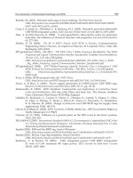
collision mechanism based on a variation of FSA. Fig. 4 illustrates EPCglobal Class-1 Gen-2
operation.
At a first stage the reader system is continuously monitoring the environment to detect the
presence of tags by means of Broadcast packets. Tags in the coverage area are excited by the
electromagnetic waves of the reader and send a reply immediately, producing a multiple
collision. The reader detects the collision and starts the identification cycle. During each
identification cycle, the time is structured as one frame, which is itself divided into slots,
following a FSA scheme.
EPCglobal Class-1 Gen-2 shows two configuration alternatives:
• Fixed frame-length procedure: All identification cycles (frames) have the same value
(number of slots). It is common to find commercial systems with this configuration.
• Variable frame length procedure (denoted as frame-by-frame adaptation). The number
of slots per frame can be changed by the reader in each identification cycle. The reader
decides if increase, decrease or maintain the number of slots per frame in function of
some criteria.
In the following subsections both procedures are overviewed, as well as the implementation
status of current readers.
3.3.1 Fixed frame length procedure
An identification cycle starts when the reader transmits a Query packet, including a field of
four bits with the value Q ∈ [0,…,15], stating that the length of the frame will be of 2
Q
slots.
Tags in coverage receive this packet and generate a random number r in the interval [0, 2
Q
-
1]. The r value represents the slot within the frame where the tag has randomly decided to
send its identification number ID=r. Inside each frame, the beginning of a slot is governed

by the reader by transmitting the QueryRep packet, excepting the slot 0, which is
automatically initiated by the Query packet. The tags in coverage use an internal counter to
track the number of transmitted QueryRep packets since the last Query packet, and then
recognize the slot when they should transmit.
When the moment arrives, the tag transmits its identification number ID, which corresponds
to the random value r calculated for contention, which is also equal to the slot number in the
frame. After transmitting its ID, three actions can follow:
- If more than one tag has chosen the same slot, a collision occurs which is detected by
the reader. Then, the reader reacts initiating a new slot with a QueryRep packet (see slot
0 in Fig. 4). The tags which transmitted their ID assume that a collision occurred, and
must update their counter value to 2
Q
-1. That means that they will not compete again in
this identification cycle.
- If the reader receives the ID correctly, and this coincides with the slot number within
the frame, then it responds with an Ack packet. All tags in coverage receive the packet
but only the identified tag answers with a Data packet, e.g. an EPC code.
If the reader receives the Data packet, it answers sending a QueryRep packet, starting a
new slot. The tag identified will finish its identification process (see slot 1 in Fig. 4).
- If the reader does not receive a correct Data packet within a given time, it considers the
time-slot has expired, and sends a Nack packet. Again, all tags in coverage receive it, but
only the tag in the identification reacts by updating its counter value to 2
Q
-1. Thus, this
tag will not contend again in this identification cycle (see slot 3 in Fig. 4). After this, the
Radio Frequency Identification Fundamentals and Applications, Bringing Research to Practice

34
reader will send a new Query or QueryRep packet to start a new frame or slot
respectively.

Finally, when a cycle finishes, a Query packet is sent again by the reader to start a new
identification cycle. Tags unidentified in the previous cycle will compete again, choosing a
new random r value.
3.3.2 Variable frame length procedure
The fixed frame length EPCglobal Class-1 Gen-2 standard provides a low degree of
flexibility. If the Q value selected is high and the number of tags in coverage is low, many
empty slots appear in the frame. On the contrary, if the Q value is low and the number of
tags is high, many collisions arise. To mitigate this problem the standard proposes a variable
frame length procedure (EPC, 2004) that selects the Q value in each cycle by means of some
arbitrary function. ((a) Bueno-Delgado et al., 2009) analyzes the different variable frame
length algorithms. Since current readers usually implement only the fixed frame length
procedure, in this chapter we focus exclusively on it.
Reader
Tag 1
Tag 2
Tag N
Query
(Q)
Slot 0
Query
Rep
Slot 1
ID=0
Collision
Ack
EPC
Slot 2
Query
Rep
Query

(Q)
Tag 3
Identification cycle
.
.
.
Slot 0
Tag
Identified
New cycle
t
Packet
error
Collision
Nack
ID=0
ID=0
ID=0
ID=2
ID=0

Fig. 4. EPCglobal Class-1 Gen-2 identification procedure
3.3.3 EPCglobal Class-1 Gen-2 in the market
The current UHF RFID readers available in the market implement the worldwide standard
EPCglobal Class-1 Gen-2. Some of them only permit to work with one of the two procedures
explained before. Besides, some readers do not permit to configure the initial frame-length
(the Q value) or only some certain values which can influence directly to the final system
performance. Depending on the level of frame-length configuration, the readers can be
classified as follows:
Characterization of the Identification Process in RFID Systems

35
• Readers with fixed frame length, without user configuration (Symbol, on-line;
ThingMagic, on-line; Mercury4, on-line; Caen, on-line; Awid, on-line; Samsys, on-line).
Identification cycles are fixed and set up by the manufacturer. It is not possible to
modify by the user (it is usually fixed to 16 slots). Therefore, these readers are not able
to optimize the frame-length.
• Readers with fixed frame length with user configuration(Samsys, on-line; Intermec, on-
line; Alien, on-line). Before starting the identification procedure the user can configure
the frame length, choosing between several values, which depend on the manufacturer.
Then, the identification cycle cannot be changed. If the user wants to establish a
different value of frame-length, it is necessary to stop the identification procedure and
restart with the new value of frame-length.
• Readers with variable frame length (Samsys, on-line; Intermec, on-line; Alien, on-line).
The user only configures the frame- length for the first cycle. Then the frame-length is
self-adjusted trying to adapt to the best value in each moment, following the standard
proposal (EPC, 2004).
4. Identification process in static scenarios
Static scenarios are characterized by a block of tags (modeling a physical pallet, box, etc.)
that enter the checking area and never leave. Two related performance measures are
commonly considered: The identification time, defined as the mean number of time units
(slots, cycles, seconds, etc.) until all tags are identified, and the system throughput or
efficiency, defined as the inverse of the mean identification time, i.e., the ratio of identified
tags per time unit.
4.1 Markovian analysis
The identification process in a static scenario is determined by the number of remaining
unidentified tags. Thus, the identification process can be modeled as a homogeneous
(Discrete Time Markov Chain) DTMC, X
c
, where each state in the chain represents the number

of unidentified tags, being c the cycle number. Thus, the state space of the Markov process is
{N, N-1,…, 0}. Fig 5 shows DTMC state diagram from the initial state, X
0
=N. The transitions
between states represent the probability to identify a certain quantity of tags t or, in other
words, the probability to have (N-t) tags still unidentified.
The transition matrix P depends on the anti-collision protocol used and its parameters. For
EPCglobal Class-1 Gen-2, the parameter K denotes the number of slots per frame (frame
length). To compute the matrix P, let us define the random variable μ
t
, which indicates the
number of slots being filled with exactly t tags. Its mass probability function is (Vogt, 2002):


Fig. 5. Partial Markov Chain
N N-1 N-2 N-t … 0 …
p
N,N-1
p
N,N-2
p
N,N-t+1-
p
N,N-t
p
N,N
N-t+1
Radio Frequency Identification Fundamentals and Applications, Bringing Research to Practice

36

,
1
(, ,)
0
Pr ( )
N
t
KN t
KNit
m
GK mN mtt
i
m
m
K
μ
−
−
−−
∏
=
==
⎛⎞
⎛⎞
⎜⎟
⎜⎟
⎜⎟
⎝⎠
⎝⎠

(1)
Where m=0, ,K and:

()
}
1
1
(,,) (1) ( )
!
1
0
l
v
ljv
i
li liv
GMlv M M j M i
v
i
i
j
⎢⎥
⎢⎥
⎣⎦
⎧⎫
−
⎧
⎛⎞
−
⎪⎪ ⎪

−
⎜⎟
=+ − − −
∑
∏
⎨⎨ ⎬
⎜⎟
=
=
⎪⎪ ⎪
⎝⎠
⎩
⎩⎭
(2)
Since the tags identified in a cycle will not compete again in the following ones, then the
transition matrix P is ((b) Bueno-Delgado et al., 2009):

,1
,
1
Pr ( ) ,
1,
,
0,
Ki
iK
iy
yi
ij iKji
ppij

ij
otherwise
μ
−
=−
⎧
=
−−≤<
⎪
⎪
=− =
∑
⎨
⎪
⎪
⎩
for i = 1,…,N. (3)
The chain has a single absorbing state, X
c
=0. The mean number of steps until the absorbing
state is the mean number of identification cycles (
c
). It can be computed by means of the
fundamental matrix, D, of the absorbing chain (Kemeny, 2009):

1
()DIF
−
=− (4)
As usual, I denotes the identity matrix, and F denotes the submatrix of P without absorbing

states. Then,

,Z
j
jB
cD
∈
=
∑
(5)
Where
B is the set of transitory states, and Z is the absorbing state.
In addition, using the physical and FSA standard parameters (Table 1 enumerates the
typical EPCglobal parameters) is possible to transform the identification time to seconds as
follows:
T
id
is the duration of a slot with a valid data transmission (EPC code). T
v
and T
c
is
the duration of an empty and collision slot, respectively. Then, the identification time in
seconds is approximated by:

total
v v c c id id
TckTkTkT
⎡
⎤

⎣
⎦
≈⋅ ⋅ + ⋅ + ⋅ (6)
v
k ,
c
k and
id
k denote the average number of empty, collision and successful slots,
respectively. These variables depend on the particular FSA algorithm and its configuration,
and on the population size. For instance, setting M=4 (see Table 1), T
id
=2.505 ms and
T
v
=T
c
=0.575 ms. Since an empty slot and a collision slot have the same duration, the
previous equation can be simplified:

[
]
ididccv
total
TkTkkcT ⋅++⋅≈ )( (7)
Characterization of the Identification Process in RFID Systems

37
Since,

vc id
kkKck
+
≈⋅− (8)
Then,

()
total
id c id id
TcKckTkT
⎡
⎤
⎣
⎦
≈⋅ ⋅− + ⋅
(9)
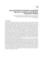
Different populations of tags and
Q values have been considered and the identification time
has been measured. Fig. 6 shows the mean number of slots required to identify each tag
population.
4.2 System throughput
The throughput (th) can be computed from the previous Markov analysis, just as the inverse
of the identification time. Another way is described in this section. Let us remark that,
obviously, the result of both methods is equal, and the second one is provided for
completeness. Given
N tags, and K slots, the probability that t tags respond in the same
time-slot is binomially distributed:

11
Pr( ) 1

tNt
N
t
t
KK
⎛⎞
⎛⎞⎛ ⎞
⎜⎟
⎜⎟⎜ ⎟
⎜⎟
⎝⎠⎝ ⎠
⎝⎠
−
=− for t=0, ,N (10)
Then, Pr(t=0) is the probability of an empty slot, Pr(t=1) the probability of a successful slot,
and Pr(t ≥2) the probability of collision:

1
Pr( 0) 1
N
t
K
⎛⎞
⎜⎟
⎝⎠
==−
(11)

1
1

Pr( 1) 1
K
N
N
t
K
⎛⎞
⎜⎟
⎝⎠
−
== − (12)

1
Pr( 2) 1 Pr( 0) Pr( 1) 1 1 1
1
N
N
ttt
KK
⎛⎞⎛ ⎞
⎜⎟⎜ ⎟
⎝⎠⎝ ⎠
≥=−=−==−− −
−
(13)
Since every identification cycles is composed by
K slots, the throughput per slot is computed
as follows:

1

1
Pr( 1) 1
N
th K t N
K
⎛⎞
⎜⎟
⎝⎠
−
=⋅ = = − (14)
4.3 Optimum Q configuration
As seen in the previous sections, the identification performance depends on the number of
tags competing and on the frame length. The best throughput performance occurs when
there are as many competing tags as slots in the frame,
N=K, yielding a maximum

Radio Frequency Identification Fundamentals and Applications, Bringing Research to Practice

38

Parameter Symbol Value
Electronic Product Code EPC 96 bits
Initial Q value
Q
0

4
Reference time interval for a
data-0 in Reader-to-Tag
signaling

TARI 12.5us
Time interval for a data-0 in
Reader-to-Tag signaling
DATA0 1.0·TARI
Time interval for a data-1 in
Reader-to-Tag signaling
DATA1 1.5·TARI
Tag-to-Reader calibration
symbol
Trcal 64us
Reader-to-Tag calibration
symbol
RTcal 31.25us
Divide Ratio DR 8
Backscatter Link Frequency LF DR/Trcal
Number of subcarrier cycles per
symbol in Tag-to-Reader
direction
M 1,2,4,8
Reader-to-Tag rate Rtrate 64Kbps
Tag-to-Reader Rate Trrate LF/M
Link pulse-repetition interval T
pri
1/LF
Tag-to-Reader preamble TÆR Preamble 6 T
pri

Tag-to-Reader End of Signaling TÆR EoS 2 T
pri

Delimiter 12.5us
Reader-to-Tag Preamble
RÆT Preamble
(RTP)
Delimiter+DATA0+TRcal+Rtcal
Reader-to-Tag Frame
synchronization
RÆT FrameSync RTP –Rtcal
Time for reader transmission to
tag response
T
1
Max(RTcal, 10 T
pri
)
Time for tag response to reader
transmission
T
2
5 T
pri

Time a reader waits, after T
1
,
before it issues another
command
T
3
5 T

pri

Minimum time between reader
commands
T
4
2·Rtcal
Query packet 22 bits 22 bits
QueryAdjust packet 9 bits 9 bits
QueryRep packet 4 bits 4 bits
Ack packet 18 bits 18 bits
Nack packet 8 bits 8 bits

Table 1. Typical values of EPCglobal Class-1 Gen-2 parameters
Characterization of the Identification Process in RFID Systems

39
throughput of 1/e ≈ 0.36 (Schoute, 1983). For EPCglobal Class-1 Gen-2,
K can not be set to
any arbitrary natural number, but to powers of two,
i.e. K=2
Q
, for Q ∈ [0, …, 15]. For every N
value, the value of
Q that maximizes the throughput has been computed in ((b) Bueno-
Delgado, 2009). Fig. 7 shows the results, and Table 2 summarizes them.
The former optimal configurations are useful for variable length readers. Readers with fixed
frame length can be optimized as well, setting the best value of
Q for a given population
size. Notice that both criteria are different: the first one optimizes the reading cycle by cycle,

whereas the second one minimizes the whole process duration. These values have been
calculated by means of simulations in ((b) Bueno-Delgado, 2009), and are also shown in
Table 2.
5. Identification process in dynamic scenarios
Many real RFID applications (e.g. a conveyor belt installation) work in dynamic scenarios.
For this type of systems, the performance analysis must be linked with the
Tag Loss Ratio.
This parameter measures the rate of unidentified tags in an identification process and,
depending on the final application, even a low TLR (
e.g. TLR=10
-3
) may be disastrous and
cause thousands of items lost per day. In this section, the TLR is computed for a RFID
scenario similar to the one depicted in Fig. 1. There is an incoming flow of tags entering the
coverage area of a reader (RFID cell), moving at the same speed (
e.g., modeling a conveyor
belt). Therefore, all tags stay in the coverage area of the reader during the same time.
Every tag unidentified during that time is considered lost. As in the previous analysis, once
acknowledged, a tag withdraws from the identification process. This problem has been
studied previously in (Vales-Alonso
et al., 2009). Thereafter, the following notation and

20 40 60 80 100 120 140 160
0
100
200
300
400
500
600

700
Tags in the coverage area (N)
Average number of slots
Q=3, 8 slots
Q=4, 16 slots
Q=5, 32 slots
Q=6, 64 slots
Q=7, 128 slots
Q=8, 256 slots
Q=9, 512 slots

Fig. 6. Mean identification time (in number of slots) vs. N, for different Q values
Radio Frequency Identification Fundamentals and Applications, Bringing Research to Practice

40
10
0
10
1
10
2
0
0.05
0.1
0.15
0.2
0.25
0.3
0.35
0.4

Tags in the coverage area (N)
Identification rate
Q=2, 4 slots
Q=3, 8 slots
Q=4, 16 slots
Q=5, 32 slots
Q=6, 64 slots
Q = 7, 128 slots

Fig. 7. Throughput (Identification rate) vs. N for different Q values


Cycle by cycle optimization Whole process optimization
Optimal
Q
Number of slots
(K)= 2
Q

Tags in coverage
(N)
Number of slots
(K)= 2
Q

Tags in coverage
(N)
1 2 N
≤
2 2 N ≤ 4

2 4 2
≤
N < 4 4 4 ≤ N < 8
3 8 4
≤
N < 9 8 8 ≤ N < 19
4 16 9
≤
N < 20 16 19 ≤ N < 38
5 32 20
≤
N < 42 32 38
≤
N < 85
6 64 42
≤
N < 87 64 85 ≤ N < 165
7 128 87
≤
N < 179 128 165 ≤ N < 340
8 256 179
≤
N < 364 256 340 ≤ N < 720
9 512 364
≤
N < 710 512 720 ≤ N < 1260
10 1024 710
≤
N < 1430 1024 1260 ≤ N < 2855
11 2048 1430

≤
N < 2920 2048 2855
≤
N < 5955
12 4096 2920
≤
N < 5531 4096 5955
≤
N < 12124
13 8192 5531
≤
N < 11527 8192
12124 ≤ N <
25225
14 16384
11527
≤
N <
23962
16384
25225 ≤ N <
57432
15 32768 23962
≤
N 32768 57432 ≤ N
Table 2. Throughput Maximization
Characterization of the Identification Process in RFID Systems

41
conventions are used: a row vector is denoted as

V
G
, the i-th component of a vector is
denoted (
V
G
)
i
, and σ(
V
G
) denotes the sum of the values of the components of a vector
V
G
.
For the sake of simplicity, let us assume tags remain
C complete cycles in the reading area.
Then, once a tag has entered the coverage area, it should be identified in the following C
identification cycles. Otherwise (if it reaches the cycle
C+1), tag is lost.
A truncated Poisson distribution, with parameter
λ, has been selected as the arrival process
in the system:

0
()
!
!
t
t

H
i
at
t
i
λ
λ
=
=
∑
(15)
For t=, ,H, being H the maximum number of tags entering per cycle.
The former assumptions allow to express the dynamics of the system as a discrete model,
evolving cycle by cycle, such that,
•
Each tag is in a given reading cycle in the set [1, ,C]
•
After a cycle, identified tags withdraw from the identification process.
•
After a cycle, each tag unidentified and previously in the i-th cycle moves to the (i+1)-th
cycle.
•
If a tag enters cycle C+1, it is considered out of the range of the reader, and, therefore,
lost.
•
At the beginning of each cycle, up to H new tags are assigned to cycle 1, following a
truncated Poisson distribution.
For any arbitrary cycle, the evolution of the system to the next cycle only depends on the
current state. Thus, a DTMC can be used to study the behavior of the RFID system. Next
section describes this model.

5.1 Markovian analysis
Based on previous considerations, the system can be modeled by a homogeneous discrete
Markov process X
c
, whose state space is described by a vector E
G
= {e
1
, , e
C+1
}, where each
e
j
∈[0, ,H], representing the number of unidentified tags in the j-th cycle. The following
figures illustrate the model. They describe the state of the system for two consecutive cycles,
showing tags entering and leaving the system, in both identification and no identification
scenarios. Therefore,
e
j
is the number of tags which are going to start their j-th identification
cycle in coverage.
e
1
component also represents the number of tag arrivals during the
previous identification cycle (which do not contend since they have not received a
Query
packet yet). Finally, component
e
C+1
indicates the number of tags lost at the end of the

identification cycle, since tags leave coverage area after
C+1 cycles.
In addition, let us define the mapping Ψ as a correspondence between the state vector and
an enumeration of the possible number of states:

[][]
()
{}
()
1
(1)
1
1
12 1
1
: 0, , 0, , 1, , 1
, , , : 1
C
C
C
j
Cj
j
HHH
Eee e E eH
+
+
+
−
+

=
⎡
⎤
Ψ××→+
⎣
⎦
=→Ψ=+
∑
GG
(16)
Radio Frequency Identification Fundamentals and Applications, Bringing Research to Practice

42
This allows defining i-th state in our model as the state whose associated vector is given by
Ψ
−1
. Let us denote
i
E
G
as the vector associated to i-th state, i.e.,
i
E
G
= Ψ
−1
(i). Finally, let e
ij

denote to the

j-th component of the
i
E
G
state vector.
The goal is to describe the transition probability matrix
P for the model, from every state i to
another state
j. The stationary state probabilities is computed as
π
G
=
π
G
P. Let us denote λ
j
as
the average incoming unidentified tags to cycle
j, which can be computed as:

1
(1)
1
C
H
j
i
j
i
j

e
λ
π
+
+
=
=
∑
G
(17)
Obviously,
λ
1
is the average incoming traffic in the system and λ
C+1
is the average outgoing
traffic of unidentified tags. Then, TLR can be calculated as:

1
)1(
1
)1(
1
1
1
λ
π
λ
λ
∑

+
+
=
+
+
⋅
==
C
H
i
i
C
i
C
e
TLR
G
(18)
To build the transition probability matrix
P let us define the auxiliary vectors
i
L
G
and
i
U
G
as:

1

{ , , }
ii iC
Le e=
G
(19)
2(1)
{ , , }
ii iC
Ue e
+
=
G

That is, the
i
E
G
state vector without either the last or the first component. Let us define the
outcome vector as:


1
(){}
i
j
i
j
i
j
i

j
C
OLU oo=− =
G
G
G
(20)
Figures 8 and 9 graphically show this computation. To construct the transition matrix let us
define the function id(i,j) that operates on an outcome vector
i
j
O
G
providing the number of
identified tags in a transition from a state i to a state j:

(, ) 1
ij
id i j O
′
=
⋅
G
G
(21)
Notice that, for
i
E
G
and

j
E
G
, if e
ik
<e
j(k+1)
for some k=1, ,C, such transition is impossible (new
tags cannot appear in stages other than stage 1). These impossible transitions will result in
id(i,j) providing a negative value. The random variable s(K,N) indicates the number of
contention slots being filled with a single tag. The
mass probability function of s(K,N) has been
computed in (Vogt, 2002) (see equation (1) and (2)). Henceforth, let us denote
Pr{s(K,N)=k} as
s
k
=(N,K)
.

As stated in section 4.2, using FSA, up to
K tags may be identified in a single identification
cycle. Therefore, possible cases range from
id(i,j)=0 to id(i,j)=K. The probability of id(i,j)
successful identifications is uniformly distributed among the contenders, whose distribution
depends on the particular state, and hence the transition probability. From equations (1) and
(2) and the previous definitions, the transition matrix
P can be computed as follows:
Characterization of the Identification Process in RFID Systems

43

10
1
,
1(,)
()(,) ,(,)0
() (,) ,(,)[1,]
(, )
0,
j
C
ik
ij
k
ij
k
jidij
ae s KN idi j
e
p
o
ae s KN idi j K
N
id i j
otherwise
=
⎧
⎪
=
⎪

⎪
⎪
⎛⎞
⎪
⎪
⎜⎟
=
⎨
⎝⎠
∈
⎪
⎛⎞
⎪
⎜⎟
⎪
⎝⎠
⎪
⎪
⎪
⎩
∏
(22)




Fig. 8. Representation of the transition state. Case 1: No identification

Fig. 9. Representation of the transition state. Case 2: Identification
Radio Frequency Identification Fundamentals and Applications, Bringing Research to Practice

44
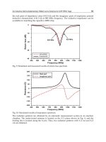
5.2 Experimental evaluation: a postal mail control system
From a practical point of view, TLR evaluation may become critical in some realistic
scenarios. As an example, this section evaluates a postal mail control system, where mails
are carried over conveyor belts for distribution, with an attached tag.
Two configurations for the mail sojourn times of 2 and 3 identification cycles have been
considered, for a frame length of
K=8 slots. The slot time is assumed to be 4 ms based on
parameters shown in Table 1. Therefore, the time sojourn is around 64 ms for
C=2 and 100
ms for
C=3. λ

range spans from 1 to 7. Results are provided in figures 10 and 11. As
expected, for a fixed C
, TLR increases as the maximum number of arrivals H increases. In
addition, for the parameters analyzed, keeping fixed
H decrements TLR if C grows, because
there are more opportunities for identification. For example, the maximum number of tags
for
H = 6 and C=2 is 12 tags, whereas for H = 6 and C=3 there might be up to 18 tags.
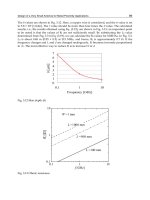
The main issue of the previous analysis is that it becomes computationally unfeasible for
moderate values of
H and C. In this case, simulation is mandatory. Figure 12 shows
simulations performed for λ=[10, ,60] and H = [3; 6]. In this case, envelopes sojourn time is
close to 800ms. We can observe that, if we set

H=3, TLR reaches 10
-4
and does not vary,
independently of the λ value. On the other hand, with
H=6, the TLR reaches up to 10
-3
. It
means that, one out of a thousand envelopes will be lost, showing the impact in the final
system.
In summary, last section allows the evaluation of TLR for different protocol parameters,
such as the number of slots, the arrival process, the time in coverage (conveyor belt
velocity),
etc.



Fig. 10. TLR results for FSA with 8 slots and Poisson arrivals. C=4, and H=3 to H=6
Characterization of the Identification Process in RFID Systems

45

Fig. 11. TLR results for FSA with 8 slots and Poisson arrivals. C=5, and H=3 to H=6


Fig. 12. TLR results for FSA with 64 slots and Poisson arrivals, C=4 and H=3, H=6
Radio Frequency Identification Fundamentals and Applications, Bringing Research to Practice

46
6. Conclusions and open issues
This chapter has presented an overview of the RFID identification process and how the

RFID systems work in
static and dynamic scenarios. The latter are common in traceability,
inventory control,
etc. Studying the identification process is mandatory to minimize the
items that leave the checking areas unidentified. Since collisions are the main factor that
produces delay in the RFID identification process, the chapter overviews this phenomenon
in the
Medium Access Control (MAC) layer. The study has been been addressed for passive
RFID protocols due to their high market penetration.
The lack of standardization has traditionally been one of the limiting factors for the
adoption of RFID technology. This situation has undergone an evolution during the last
years, since the EPCglobal Class-1 Gen-2 standard have been widely accepted by RFID
companies. The more relevant and adopted EPCglobal specifications have been described
along the chapter, in particular, its physical and its anti-collision protocol.
The performance analysis of the identification process has been introduced. On the one
hand, the analysis has been focused on
static scenarios, where identification time has been
computed, as well as system throughput. On the other hand, the identification process
analysis of
dynamic scenarios has been oriented to determine the Tag Loss Ratio.
Configuration of actual implementations of RFID systems could make use of the results
achieved to improve their identification process quality.
Finally, some open issues related to identification procedure have not been addressed yet:
the analytical characterization of DFSA algorithms, more complex incoming traffics for
dynamic systems, as well as considering another types of collisions, such as reader to reader.
The study of these issues will be important in the research field of RFID for the next years.
7. Acknowledgments
This work has been supported by project grant DEP2006-56158-C03-03/EQUI, funded by the
Spanish Ministerio de Educacion y Ciencia, projects TEC2007-67966-01/TCM (CON-PARTE-
1), TSI-020301-2008-16 (ELISA) and TSI-020301-2008-2 (PIRAmIDE), funded by the Spanish

Ministerio de Industria, Turismo y Comercio and partially supported by European Regional
Development Funds. It has been also developed within the framework of "Programa de
Ayudas a Grupos de Excelencia de la Región de Murcia", funded by Fundación Seneca,
Agencia de Ciencia y Tecnologia de la Región de Murcia (Plan Regional de Ciencia y
Tecnologia 2007/2010).
8. References
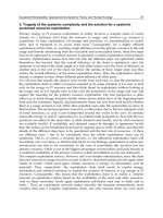
Angerer, C., Maier, G., Bueno-Delgado, M.V., Rupp, M., Vales-Alonso, J. (2010), Recovering
from Collisions in Multiple Tag RFID Environments
. In Proc. of International
Conference on Industrial Technology, Viña del Mar, Chile.
(a) Bueno-Delgado, M.V., Vales-Alonso, J., Gonzalez-Castaño, F.J. (2009),
Analysis of DFSA
Anti-Collision Protocols in passive RFID environments
. In Proc. of 35
th
Annual
Conference of the IEEE Industrial Electronic Society. pp. 2630-2637.
(b) Bueno-Delgado, M.V., Vales-Alonso, J., Egea-Lopez, E., Garcia-Haro, J (2009),
Optimum
Frame-length configuration in passive RFID systems installations.
In Proc of
Characterization of the Identification Process in RFID Systems

47
International Workshop on RFID Technology, Concepts, Applications and
Challenges. Milan, Italia. pp. 69-77.
EPC Radio-Frequency Identify protocol for communications at 868–960 MHz,Version 1.0.9:
EPCglobal Standard Specification, 2004. Available Online at:

Finkenzeller, K., (2003) RFID Handbook

: Fundamentals and Applications in Contactless Smart
Cards and Identification
, chapters 1–2, 1-7,11-28. 2
nd
Edition, John Wiley and Sons,
Chichester. New York.
Hush, D.R. and Wood, C. (1998),
Analysis of tree algorithms for RFID arbitration. In Proc. of
IEEE International Symposium on Information Theory.
ISO/IEC 1800–6:2003(E), Part 6: Parameters for Air Interface Communications at 860–960
MHz.
Jacomet, M., Ehrsam, A. and Gehring, U. (1999),
Contactless identification device with anti-
collision algorithm
. In Proc. of IEEE Conference on Circuits, Systems, Computers and
Communications, Athens, Greece, pp. 269–273.
Kemeny, J. G., & Snell, J. L. (1960).
Finite Markov chains. Princeton, NJ: D. Van Nostrand
Company, Inc.
Khasgiwale, R.S., Adyanthaya, R:U., Engels, D.E. (2009),
Extracting Information from tag
collisions
. In Proc. of IEEE International Conference on RFID, Orlando USA.
Law, C., Lee, K. and Siu, K. (2000),
Efficient memoryless protocol for tag identification. In Proc. of
the 4th International Workshop on Discrete Algorithms and Methods for Mobile
Computing and Communications,. Boston, Massachusetts,pp. 75–84.
Leon-Garcia A. and Widjaja, I. (1996),
Communication Networks: Fundamental Concepts and Key
Architectures

, McGraw-Hill, Press, Boston, Chapter 6, part 1, 368-421.
Myung, J. and Lee, W. (2006),
Adaptative binary splitting: A RFID tag Collision arbitration
protocol for tag identification
, Mobile Networks and Applications Journal, 11, pp.
711–722.
Schoute, F.C., (1983),
Dynamic frame length ALOHA, IEEE Transactions on Communications,
31(4), 565–568.
Shen, D., Woo, G., Reed, D.P., Lippman, A.B., Wang, J. (2009),
Separation of Multiple Passive
RFID Signals Using Software Defined Radio
. In Proc. of IEEE International Conference
on RFID, Orlando USA.
Shih, D.H., Sun, P.L., Yen, D.C., Huang S.M. (2006),
Taxonomy and survey of RFID anti-
collision protocols
, Elsevier Computer Communications, 29, 2150–-2166, 2006.
Vales-Alonso, J, Bueno-Delgado, M.V., Egea-Lopez, E., Alcaraz-Espin, J.J, Garcia-Haro, J.
(2009),
Markovian Model for Computation of Tag Loss Ratio in Dynamic RFID Systems.
In Proc. of 5th European Workshop on RFID Systems and Technologies, RFID
SysTech, Bremen, (Germany).
Weselthier, J.E., Ephremides, A., and Michaels, L.A. (1988),
An exact analysis and performance
evaluation of framed ALOHA with capture.
IEEE Transactions on Communications, 37
(2), pp. 125–137.
William J. Stewart,
Introduction to the Numerical Solution of Markov Chains. Princeton

University Press.
On-line references:
Awid, RFID Reader. Documentation available on-line at:
Radio Frequency Identification Fundamentals and Applications, Bringing Research to Practice

48
Caen, RFID Reader. Documentation available on-line at:

Intermec, RFID Reader. Documentation available on-line at: .
Impinj, RFID Reader. Documentation available on-line at: .
Samsys, RFID Reader. Documentation available on-line at:
Symbol, RFID Reader. Documentation available on-line at: http:// www.tecno-
symbol.com/
ThingMagic Mercury4, RFID Reader. Documentation available on-line at:



3
The Approaches in Solving Passive RFID
Tag Collision Problems
Hsin-Chin Liu
National Taiwan University of Science and Technology
Taiwan
1. Introduction
Radio Frequency Identification (RFID) systems are being intensively used recently for
automated identification. Every object can be detected as one form of an electronic code. At
the beginning, the main purpose of RFID tag usage is meant to be an improvement of
barcodes. Besides the fact that an RFID tag does not need line of sight to obtain its ID, the
tag is also water and dirt resistant. Moreover, it also has a read-and-writable memory chip,
which can store much more data than a barcode, and is difficult to be imitated. The above

are the main factors that many enterprises and government associations consider to
extensively apply the RFID technology to many applications.
An RFID tag is composed of two major components: an IC to store data and to handle
communication processing and an attached antenna to transmit and receive radio signal.
There are several types of RFID tags based on the differences of their power sources and
communication methods. In general, a passive RFID tag does not have an internal power
supply, and cannot work without collecting continuous wave from a reader. Oppositely, an
active RFID tag has an attached battery and can communicate with other tags or reader on
its own. A semi-passive tag is a mixed of above two types, which has an external battery for
its operating power and yet communicates with reader in the same way as a passive tag
does.
In an RFID system, a reader is able to communicate with many tags within its coverage.
However the tag identification process may fail when multiple tags are sending their data
simultaneously. The signals from the tags may interfere with each other and hence the
reader may not receive any correct data at all. If this happens, the tags will have to
retransmit their data, which wastes the tag reading time and hence degrades the system
performance. Such a problem is often called “tag collision” in an RFID system.
To overcome the tag collision problem, researchers are still looking for the most effective
anti-collision method to achieve high speed detection with nearly 100% data accuracy ID
retrieval. The collision problems are usually classified into two types: the reader collision
problems and tags collision problems (Burdet 2004; Dong-Her Shih 2006; Okkyeong Bang
2009). In this chapter, we focus on the latter one.
The tag collision problems are in conjunction with the anti-collision protocols used in
various RFID systems, of which the objective is to retrieve a tag’s ID accurately with low
transmission power, low computational complexity, and minimum time delay. In the
Radio Frequency Identification Fundamentals and Applications, Bringing Research to Practice

50
following we will overview a variety of anti-collision methods in solving RFID tag collision
problems. Unlike many other surveys of RFID anti-collision methods that are mostly

focusing on Time Division Multiple Access (TDMA) schemes, this work elaborates more
details of applying other multiple access technologies to the passive RFID systems.
2. Review of anti-collision schemes for passive RFID systems
Multiple access technologies are extensively used to allow multiple communications to
coexist in the communication channel with little interference with each other in modern
communication systems. In an RFID system, a reader usually communicates with many tags
within its read range, which means that all the reader and tag communications share the
same air medium as their communication channel. Thus a variety of multiple access
technologies have been used in recent RFID systems, such as Time Division Multiple Access
(TDMA), Code Division Multiple Access (CDMA), Spatial Division Multiple Access
(SDMA), Frequency Division Multiple Access (FDMA), and the hybrid multiple access
technologies. In the following, we overview the multiple access technologies that have been
proposed. Fig. 1 illustrates the category of multiple access schemes used in different RFID
systems.



Fig. 1. Map of tag anti-collision schemes in RFID system
The Approaches in Solving Passive RFID Tag Collision Problems

51
2.1 Time Division Multiple Access (TDMA) based schemes
With the TDMA technology, the reader and tag communications can use the same frequency
in the same reader coverage, and each tag response can be differentiated by the time interval
that it used. This kind of multiple access technology is the most popular RFID tag anti-collision
schemes and can easily jointly incorporate with other multiple access technologies. As seen in
Fig. 1, the RFID tag anti-collision schemes using TDMA technologies can be divided into two
categories, the deterministic schemes and the probabilistic schemes (V. Sarangan 2008). The
deterministic schemes are usually referred to as binary tree-search based schemes. The
schemes are deterministic because each root-to-leaf path denotes a unique tag ID and all IDs

can be retrieved once all branches are completely searched. On the other hand, the
probabilistic schemes are usually referred to as slotted ALOHA based schemes. Each tag ID in
the probabilistic schemes will have a chance to be retrieved successfully; however, there is a
possibility that some tags may not be accessed due to recurrent collisions. Other than the
above two categories, some hybrid schemes are also proposed; for instance, Bonuccelli et al.
proposed a tree slotted ALOHA (TSA) is proposed in (Bonuccelli et al. 2006), and Shin et al.
also proposed another hybrid tag anti-collision scheme (Shin et al. 2007).
Because the fundamental binary tree-search scheme interrogates one branch completely to
obtain a tag ID, it is naturally slow. Let L(N) denote the average number of iterations that
are required to retrieve one tag ID among N tags. The L(N) can be calculated as Eq. (1)
(Finkenzeller 2004).
L(N) = log
2
N + 1 (1)
Obviously the value L(N) becomes large when there are many tags in the reader’s coverage.
Hence, a variety of tree-search schemes have been proposed to mitigate this problem. The
tree-search schemes are further categorized into two major types: Binary Tree Walking
schemes and Query Tree schemes (Dong-Her Shih 2006; Okkyeong Bang 2009).
Compared with the tree-search scheme, the slot ALOHA schemes usually interrogate tags
faster. Because slotted ALOHA scheme segments the reader and tag communications into
many time slots. Each time slot can be empty (which means no tag response in the time slot),
collided (which means multiple tag responses in the time slot), or successful (which means
exactly one tag response in the time slots). Because using a pure TDMA scheme, only one
tag response can be read by the reader in a time slot. The performance of the schemes is
hence determined by the probability of occurrence of a successful time slot. The probability
of observing a successful time slot P
succ
can be written as Eq. (2).

1

11
1,
tag
n
succ tag
frame frame
Pn
nn
−
⎛⎞⎛ ⎞
⎜⎟⎜ ⎟
=−
⎜⎟⎜ ⎟
⎝⎠⎝ ⎠
(2)
where the n
tag
denotes the number of tags in the reader’s coverage, and n
frame
denotes the
number of slots that a tag can select, which is also called as a frame size. When the number
of tags in the reader’s coverage is large, it is reasonable to assume that the distribution of the
probability of receiving a tag response is a Poisson distribution. Under such a circumstance,
the optimal system performance (or throughput) of a slotted ALOHA scheme can achieve as
36.8% (that is, MAX(P
SUCC
)= 36.8%) when n
frame
= n
tag

(Proakis 1995; Finkenzeller 2004).
Apparently, the ratio of the frame size to the number of tags in the reader’s coverage
determines the system throughput. As the amount of tags that needs to be read is unknown
Radio Frequency Identification Fundamentals and Applications, Bringing Research to Practice

52
in advance for most cases, to choose a proper frame size is a key factor that can determine
the system performance. Moreover, the proper frame size is usually time-variant because
the number of unread tags decreases in an inventory process, which gives a challenge on
choosing the most suitable frame size (Wang & Liu 2006). Since several papers have
addressed this kind of research comprehensively (Dong-Her Shih 2006; Okkyeong Bang
2009), we will not describe further details on the TDMA schemes in this chapter but refer
readers to those papers.
2.2 Code Division Multiple Access (CDMA) based schemes
As mentioned earlier, the TDMA based anti-collision schemes can only retrieve one tag’s ID
at one time slot. In order to significantly increase the system throughput, incorporating the
TDMA technology with other multiple access technology is necessary.
The CDMA technology has been extensively used in many modern communication systems.
The CDMA schemes allow multiple communications to coexist in the same medium using
the same time and frequency resources. The CDMA technology is usually categorized into
two types: frequency hopping CDMA (FH-CDMA) and direct sequence spreading CDMA
(DS-CDMA). Because a passive tag is unable to select the communication frequency actively
but only backscatters the radio signal emitted from a reader, the FH-CDMA technology is
hence not suitable for the passive RFID system. The DS-CDMA technology however uses a
spread sequence as the signature of a signal source. Different signal sources can transmit
their signals at the same time, and the receiver is able to separate each signal from the
received signals by dispreading the received signals with its corresponding signature.
There are a variety of spreading sequences for different DS-CDMA applications. The
sequences are generally separated into two groups. One is called “orthogonal sequences”,
and the other is called “pseudo random sequences”. For instance, the well-known Walsh

code is one of the orthogonal sequences and another well-known Gold code is one of widely
used pseudo random sequences. Most orthogonal sequences require perfect synchronization
(that is, each code should arrive at the receiver at the same time) to preserve their mutual
orthogonality. On the other hand, the perfect synchronization is not required for pseudo
random sequences to be low cross-correlated; however, the pseudo random sequences are
not mutually orthogonal. Due to the low cross-correlation value, a near-far problem can be
caused if the received powers from the signal sources are different. Another kind of
spreading sequence is called shift-orthogonal sequences. A shift-orthogonal sequence can
maintain orthogonality with a different shift-orthogonal sequence and with a delayed
version of itself. Thus, the sequences do not require synchronization and can resist the near-
far effect. A Huffman sequence is one example of the shift-orthogonal sequences.
A passive tag can generate a desired signal by changing its antenna reflection coefficient to
produce the proper backscatter signal. This is usually referred to as backscatter modulation.
Using the backscatter modulation, the tag can easily produce a desired coded signal.
Several studies on using CDMA technology onto RFID systems have been revealed
(Fukumizu et al. 2006; Rohatgi 2006; Wang et al. 2006; Maina et al. 2007; Liu and Guo 2008).
Rohatgi and Wang et al. both proposed methods of applying Gold sequences to RFID
systems. However, due to the non-zero cross-correlation of each spreading sequence, the
performance of this method deteriorates when there exists power inequality amount the tag
backscatter signals. In general, a passive tag merely returns its response by backscattering
the incident continuous wave, which is emitted from a reader. The strength of a received tag
backscatter signal is determined by a variety of factors, including the power of the incident