Volume 21 - Composites Part 6 pdf

Livermore, CA
MSC-
NASTRAN/DYTRAN
MSC Software
Corp., Costa Mesa,
CA

VR&D-GENESIS Vanderplaats
Research &
Development, Inc.,
Colorado Springs,
CO

Pre- and postprocessors
PATRAN MSC Software
Corp., Costa Mesa,
CA

HyperMesh Altair
Engineering, Inc.,
Troy, MI

The pre- and postprocessors of most of the commercial codes listed in Table 2 support the key aspects related to
the analysis of fibrous composite materials. These include:
• Input of ply properties based on unidirectional as well as 2-D woven fiber architecture
• Ply lay-ups
• Vector orientations used to define ply orientation in space
• Computation of 3-D effective properties
• Computation of [A], [B], and [D] stiffness matrices for plate and shell elements
• Recovery of strains and stresses in various coordinate systems, such as global axis, local element axis,
laminate axis, and lamina axis

• First ply failure based on either point stress/ strain (maximum strain/stress) or quadratic failure (Tsai-
Wu, Hill, Hashin) criterion
Some of the explicit analysis codes, such as LS-DYNA, MSC-DYTRAN, PAM-CRASH, and ABAQUS also
provide progressive damage material models for ultimate failure load prediction. However, these computational
progressive damage models have not been experimentally verified for a wide variety of structural applications.
Based on the author's personal experience, ESI-SYSPLY is perhaps the most comprehensive and user-friendly
pre- and postprocessor program currently available for composite FEA. However, in the current form, it does
not have the interface with most widely used FEA solvers, such as NASTRAN and ABAQUS, thereby severely
limiting its utility. Over the years pre- and postprocessing tools have been highly optimized for the FEA of
metallic structures. These tools now need significant enhancement in their capabilities to accurately and
efficiently analyze and design complex structures manufactured from advanced composite materials.
Reference cited in this section
4. J.M. Whitney, Structural Analysis of Laminated Anisotropic Plates, Technomic, 1987

Finite Element Analysis
Naveen Rastogi, Visteon Chassis Systems

Numerical Examples
The continuity of transverse stresses at the layer interfaces and the free-edge effects are unique aspects in the
analysis of multilayered composite structures. Finite element analysis of two classical examples from the
mechanics of composite materials illustrates these aspects of multilayered composite structures. The first
example is a problem of transverse bending of a simply supported [0/90/0]
T
laminated plate, the benchmark
solution of which was obtained by Pagano (Ref 30). The second numerical example is of a [0/90]
s
laminated
plate under uniform extension (Pagano, Ref 31, 32), illustrating the free-edge effects in multilayered composite
structures.
Example 1: Transverse Bending of a Laminated Plate. A simply supported [0/90/0]

T
laminated plate is
subjected to sinusoidal loading on the top surface. Laminated plates with two different aspect ratios are
considered. For a/h= 4, the plate represents a thick multilayered structure. For a/h= 50, a thin-walled structure
is represented. All layers are assumed to be of equal thickness. The material properties for the orthotropic
lamina are (Ref 30): E
1
/E
2
= 25, E
2
=E
3
, G
12
/E
2
=G
13
/E
3
= 0.5, G
23
/E
2
= 0.2, ν
12
=ν
13
=ν

23
= 0.25. The origin of the
right- handed coordinate system is chosen at the corner of the middle surface of the plate, that is, 0 ≤x≤a, 0
≤y≤b, and–(h/2) ≤z≤ (h/2) (see Fig. 6).

Fig. 6 A simply supported [0/90/0]
T
laminate subjected to sinusoidal loading on the top
surface
This problem is analyzed by using the novel 3-D FEA tool SAVE, developed by the author (Ref 21, 22). For
the laminated plate problem described previously, a quick comparison between 3-D elasticity solution of
Pagano (Ref 30) and the 3-D structural analysis code SAVE is presented in Table 3 for various a/h ratios. The
normalized quantities used in Table 3 are described as: , ,
, , , , where s=a/h and q
0
is the
peak magnitude of the applied sinusoidal pressure load at the center of the laminated plate at the top surface.
The results presented in Table 3 demonstrate the accuracy of SAVE analysis code in the 3-D analysis of multi-
layered structures. Results from SAVE analysis can now be used as a basis to compare with the results obtained
from commercial FEA codes.
Table 3 Comparison between the results obtained for various a/h ratios for a [0/90/0]
T

simply supported laminate subjected to sinusoidal loading on the top surface
Quantity a/h= 2 a/h= 4 a/h= 10 a/h= 50 a/h= 100 Source




1.4361.436 0.8010.801 0.5900.590 0.5410.541 0.5390.539

(a)

(b)




–0.937–0.938 –0.754–0.755 –0.590–0.590 –0.541–0.541 –0.539–0.539
(a)

(b)




0.6680.669 0.5340.534 0.2840.285 0.1840.185 0.1810.181
(a)

(b)




–0.742–0.742 –0.556–0.556 –0.288–0.288 –0.185–0.185 –0.181–0.181
(a)

(b)

–0.0859–
0.0859
–0.0511–
0.0511
–0.0288–
0.0289
–0.0216–
0.0216
–0.0214–
0.0213
(a)

(b)




0.07020.0702 0.05050.0505 0.02900.0289 0.02160.0216 0.02140.0213
(a)

(b)




0.1640.164 0.2560.256 0.3570.357 0.3930.393 0.3950.395
(a)

(b)

0.25910.2591 0.21720.2172 0.12280.1228 0.08420.0842 0.08280.0828
(a)

(b)

(a) (a) From the SAVE analysis (Ref 21, 22). (b) By Pagano (Ref 30)
Next, the example problem is analyzed using commercial FEA codes such as ABAQUS (Ref 33), NASTRAN
(Ref 34), and I-DEAS (Ref 35). The solid elements—C3D8 and C3D20 in ABAQUS, and CHEXA and
CHEXA20 in NASTRAN—and linear and parabolic brick in I- DEAS are used in the analyses. Results from
the commercial FEA codes and the SAVE analysis are compared in Table 4 for a/h= 4. The mesh description
shown in Table 4 represents the number of elements that are used to represent each composite layer in the three
orthogonal coordinate directions. For example, a 12 × 12 × 2 finite element mesh represents 12 solid elements
in x- and y-direction each, and 2 solid elements in the z-direction, in every single composite layer. As is shown
in Table 4, the numerical values of the six stress components as obtained from the 3-D FEA using solid
elements with quadratic shape functions (parabolic in I-DEAS, CHEXA20 in NASTRAN, and C3D20 in
ABAQUS) are within 5% of the exact values. Only the transverse shear stress component, τ
yz
, shows some
significant difference (about 12 %) from the exact solution. However, as is shown in Table 4, the accuracy in
the solution of this stress component is increased significantly by refining the FE mesh. In Table 4, compare the
results obtained from I-DEAS and ABAQUS analyses with progressive mesh refinement (6 × 6 × 2, 12 × 12 ×
2, and 20 × 20 × 4 meshes of parabolic solid elements). It is also worth noting that a sufficiently accurate
solution to the problem being analyzed could be obtained by using parabolic brick elements in a coarse mesh (6
× 6 × 2 per layer) with 2916 DOF only. However, in spite of using a more refined mesh (12 × 12 × 2 per layer),
solid elements with linear shape functions (linear brick in I-DEAS and C3D8 in ABAQUS) do not provide an
accurate solution. For the numerical problem analyzed here, solid elements with linear shape functions, also

known as constant strain elements, can be erroneous in the bending stress values by as much as 30%.
Table 4 Comparison among the results obtained for a/h= 4 from various 3-D analyses for a [0/90/0]
T
simply supported
laminate subjected to sinusoidal loading on the top surface
Quantity SAVE, 1 ×
1 × 1,M=
6, 1,805
DOF
ABAQUS, 20
× 20 × 4,
C3D20, 61,200
DOF
ABAQUS, 12
× 12 × 2,
C3D20, 11,664
DOF
NASTRAN, 12 ×
12 × 2,
CHEXA20,
11,664 DOF
I-DEAS, 12 ×
12 × 2
(parabolic),
11,664 DOF
I-DEAS, 6 × 6
× 2 (parabolic),
2,916 DOF
I-DEAS, 12
× 12 × 2

(linear),
3,024 DOF
ABAQUS, 12
× 12 × 2,
C3D8, 3,024
DOF



1.0 1.005 1.02 1.02 1.02 1.025 0.950 0.826



0.801 0.788 0.800 0.800 0.769 0.773 0.760 0.571



–0.754 –0.744 –0.750 –0.750 –0.725 –0.729 –0.716 –0.547



0.534 0.528 0.532 0.532 0.516 0.521 0.514 0.483



–0.556 –0.550 –0.554 –0.554 –0.539 –0.543 –0.537 –0.514



–0.0511 –0.0508 –0.0509 –0.0498 –0.0500 –0.0504 –0.0492 –0.0519

0.0505 0.0503 0.0503 0.0494 0.0496 0.0500 0.0487 0.0514



0.256 0.257 0.255 0.256 0.257 0.259 0.252 0.261



0.2172 0.2228 0.2400 0.2398 0.2408 0.2427 0.1743 0.1703
DOF, degrees of freedom; M, degree of polynomial
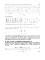
The through-the-thickness distributions of six stress components, as shown in Fig. 7, demonstrate many unique
features of the 3-D stress state in multilayered laminated composite structures. Note the jump in the in-plane
normal stress components σ
xx
and σ
yy
at the layer interfaces (see Fig. 7a and b). In multilayered laminated
structures, in-plane stresses σ
xx
, σ
yy
, and τ
xy
are discontinuous (hence, the in-plane strains
xx
,
yy

, and γ
xy
are
continuous) at the layer interfaces. On the other hand, the transverse stresses σ
zz
, τ
yz
, and τ
xz
are continuous at
the material interfaces, as shown in Fig. 7(c)–(e). However, the out-of-plane strains
zz
, γ
yz
, and γ
xz
are now
discontinuous (or jump) at these interfaces.

Fig. 7 Through-the-thickness distributions for a/h= 4. (a) σ
xx
. (b) σ
yy
. (c) σ
zz
. (d) τ
xz
. (e) τ
yz
.

(f) τ
xy
. In the legend for these curves, M is the degree of the polynomial.
Continuity of the transverse normal and shear stresses at the layer interface, is a unique and important aspect in
the analysis of multilayered laminated structures. Table 5 presents the actual numerical values of transverse
stress components σ
zz
, τ
yz
, and τ
xz
at the layer interfaces, thereby providing a deeper insight into the continuity
of these interlaminar stresses. The notation “T” represents values computed at the interface approaching from
the top; similarly, “B” represents values computed at the interface approaching from the bottom. While the
SAVE analysis code is almost perfect in satisfying the continuity of interlaminar stresses at the interfaces,
ABAQUS analysis with a very refined mesh (20 × 20 × 4 per layer with 61,200 DOF) is also reasonably good
in achieving that goal. However, as the mesh size becomes coarser, the commercial FE analyses results tend to
become more distinct as well as less accurate at the interface (refer to Table 5). Once again, in all the
commercial FE analyses, the transverse shear stress component, τ
yz
, shows the most significant differences. As
is shown in Table 5, the continuity of interlaminar stresses at the layer interfaces is the worst from the FEA
with constant strain elements, thereby making them unsuitable for transverse bending analysis of multilayered
composite structures.
Table 5 Interlaminar stresses as obtained at the ply interfaces from various 3-D analyses of a [0/90/0]
T
simply supported
laminated plate (a/h= 4) subjected to sinusoidal loading on the top surface
Quantity SAVE, 1 × 1
× 1 mesh (M=

6), 1,805
DOF
ABAQUS, 20
× 20 × 4,
C3D20,
61,200 DOF
ABAQUS, 12
× 12 × 2,
C3D20,
11,664 DOF
NASTRAN,
12 × 12 × 2,
CHEXA20,
11,664 DOF
I-DEAS, 12 ×
12 × 2
(parabolic),
11,664 DOF
I-DEAS, 6 ×
6 × 2
(parabolic),
2,916 DOF
I-DEAS, 12 ×
12 × 2
(linear), 3,024
DOF
ABAQUS, 12
× 12 × 2,
C3D8, 3,024
DOF

TB

0.2690.269 0.2670.270 0.2580.265 0.2580.265 0.2640.269 0.2660.271 0.3820.182 0.3890.099



TB

0.25750.2575 0.25750.2625 0.25750.2725 0.25750.2725 0.25750.2750 0.26000.2770 0.25330.2693 0.26130.2730



TB

0.07580.0758 0.08280.0763 0.10100.0778 0.10050.0775 0.10100.0780 0.09670.0786 0.17090.0645 0.16430.0665



TB

0.7180.718 0.7190.721 0.7190.725 0.7190.725 0.7220.726 0.7280.732 0.8080.605 0.8810.582



TB

0.25250.2525 0.25750.2525 0.27000.2525 0.27000.2525 0.27000.2525 0.27330.2548 0.27250.2508 0.26800.2618

TB

0.08930.0893 0.08980.0963 0.09100.1145 0.09100.1140 0.09150.1145 0.09220.1155 0.07500.1778 0.07380.1786
DOF, degrees of freedom; T, top; B, bottom; M, degree of polynomial
In general, a 3-D analysis using discrete layer- by-layer representation of the laminate can be performed with
reasonable accuracy, using solid elements with quadratic shape functions in any of the commercial FE codes
evaluated here. However, due to limitations in the available computational resources, many times it may not be
possible to discretize a complex, practical structure completely with 3-D solid elements. In addition, most of the
real-life structures are thin- walled, so as to justify the use of 2-D shell elements in their analyses. However, the
limitations, or bounds, of using 2-D shell elements to accurately analyze multi-layered composite structures
needs to be well understood.
The thick laminated plate problem (a/h= 4) described previously is now analyzed using 2-D shell elements
available in the commercial FE codes, namely, ABAQUS (S4R), NASTRAN (CQUAD4), I-DEAS (linear
shell), and MECHANICA (p-type shell) (Ref 36). The type of shell element used in each analysis is mentioned
in parentheses. The stress solutions obtained from various 2-D shell analyses are compared with the exact 3-D
solution, as shown in Table 6. The 2-D shell analysis does not provide the transverse normal stress component,
σ
zz
. Note the very high numerical discrepancy among the stress values as obtained from exact 3-D solution and
various 2-D analyses using shell elements. The largest discrepancy is in the magnitude of stress in the fiber
direction in 0° layer, where the stress values from the 2-D analysis are almost 50% lower than the exact 3-D
values. At the same time, the similarity among the 2-D analyses solutions is remarkable. Except for the values
of transverse shear stress, τ
yz
, as obtained from MECHANICA, the numerical results for the stresses obtained
from the 2-D shell analyses are essentially the same. A systematic attempt was made to check the convergence
of the 2-D solutions by increasing the order of shell elements (e.g., S4R to S8R in ABAQUS, CQUAD4 to

CQUAD8 in NASTRAN, and linear shell to parabolic shell in I-DEAS), as well as by refining the FE mesh in
the model. No further improvement in the numerical solution of the problem was observed.
Table 6 Comparison among the results obtained for a/h= 4 from various 2-D analyses for
a [0/90/0]
T
simply supported laminate subjected to sinusoidal loading on the top surface
Quantity SAVE (3-D),
1 × 1 × 3
mesh (M= 6)
1,805 DOF
I-DEAS (2-D),
24 × 24 mesh
(linear shell),
3,553 DOF
ABAQUS (2-
D), 24 × 24
mesh, S4R,
3,553 DOF
MECHANICA,
2-D;p= 6
NASTRAN (2-D),
24 × 24 mesh,
CQUAD4, 3,553
DOF



0.801 0.397 0.397 0.398 0.396

–0.754 –0.397 –0.397 –0.398 –0.396



0.534 0.592 0.592 0.592 0.592



–0.556 –0.592 –0.592 –0.592 –0.592



–0.0511 –0.0429 –0.0429 –0.0429 –0.0428



0.0505 0.0429 0.0429 0.0429 0.0428



0.256 0.310 0.310 0.310 0.310



0.2172 0.2750 0.2750 0.0675 0.2750
DOF, degrees of freedom; M or p, degree of polynomial
Further insight into this subject is gained by analyzing the laminated plate problem described previously with
a/h= 50. The same 2-D shell elements and FE mesh are used during the analysis. Numerical results from a
typical 2-D shell analysis using SDRC I-DEAS and the 3-D exact analysis SAVE are presented both in tabular

form (Table 7) and as plots of stress distributions through the thickness of the laminate (Fig. 8). Except for the
transverse shear stress component, τ
yz
, numerical solutions obtained from the 2-D and 3-D analyses for this
problem compare very well with each other. The numerical examples discussed here emphasize the need to
understand the limits of 2-D shell elements in the analysis of anisotropic, multi-layered composite structures.
Table 7 Comparison among the results obtained for a/h= 50 from various 2-D analyses
for a [0/90/0]
T
simply supported laminate subjected to sinusoidal loading on the top
surface
Quantity SAVE (3-D),
1 × 1 × 3
mesh, (M= 6)
1,805 DOF
I-DEAS (2-D),
24 × 24 mesh
(linear shell),
3,553 DOF
ABAQUS (2-D),
24 × 24 mesh,
S4R, 3,553 DOF

MECHANICA,
2-D;p= 6
NASTRAN, 24 ×
24 mesh,
CQUAD4, 3,553
DOF

0.541 0.536 0.536 0.536
0.536



–0.541 –0.536 –0.536 –0.536
–0.536



0.184 0.184 0.184 0.183
0.184



–0.185 –0.184 –0.184 –0.183
–0.184



–0.0216 –0.0215 –0.0215 –0.0215
–0.0215



0.0216 0.0215 0.0215 0.0215
0.0215

0.393 0.394 0.392 0.388
0.392



0.0842 0.104 0.104 0.025 0.104
DOF, degrees of freedom; M or p, degree of polynomial

Fig. 8 Comparisons between 2-D and 3-D solutions for a/h= 50. (a) σ
xx
. (b) σ
yy
. (c) τ
yz
. (d)
τ
xz
. (e) τ
xy
. In the legend for these curves, M is the degree of the polynomial.

Example 2: Uniaxial Extension of a Laminated Plate. This example focuses on the free- edge effects in a [0/90]
s

laminated plate subjected to uniaxial extension (see Fig. 9). Pagano (Ref 31) presented the closed-form solution
to this classical problem in 1974. Later on, Pagano and Soni (Ref 32) also solved this problem using a global-
local variational model. Here, the results from the SAVE FE analysis program, performed using a 1 × 20 × 12
mesh of variable- order rectangular solid elements (Ref 21, 22), are presented.

Fig. 9 A [0/90]
S
laminate subjected to uniform axial extension
Due to the symmetry of geometrical and materials properties and the applied loading, only one-eighth of the
configuration of the [0/90]
s
laminated plate (a=b= 4 h; see Fig. 9) need be analyzed. The uniform extension of
the laminated plate is achieved by applying a uniform axial displacement at the ends x=a. For the purpose of
analyses, the following lamina elastic constants are taken (Ref 31):
E
1
= 138 GPa (20 × 10
6
psi)


E
2
=E
3
= 14.5 GPa (2.1 × 10
6
psi)


G
12
=G
13

=G
23
= 5.9 GPa (0.85 × 10
6
psi)


ν
12
=ν
13
=ν
23
= 0.21

The distributions of interlaminar stresses as obtained from the analysis are plotted along the y-direction at x/a=
0.5. All the stress components are normalized by the applied axial strain. The distributions of the transverse
normal stress, σ
zz
, as obtained from the analysis at the midsurface of the [0/90]
s
laminate in the 90° layer, are
shown in Fig. 10. The normalized peak value of 2.0 GPa (0.29 × 10
6
psi) for this stress component, which
occurs at the free edge y/b= 1, compares very well with those obtained by Pagano (Ref 31) and Pagano and
Soni (Ref 32). Next, the distributions of the normalized transverse normal stress component, σ
zz
, as obtained
from the analysis at the interface of the 0/90 layers, are shown in Fig. 11. Note that in Fig. 11 the numerical

results from both 0° layer and 90° layer are plotted separately but appear superimposed. As is shown in Fig. 11,
the continuity of the transverse normal stress component, σ
zz
, is satisfied extremely well. Similar observations
are made regarding the distributions of the transverse shear stress component, τ
yz
, as shown in Fig. 12. Note the
high gradients of interlaminar stresses that occur in the vicinity of the free-edge at y/b= 1 (see Fig. 11 and 12).
These stresses are normally the primary cause of delamination failure in multilayered laminated structures.

Fig. 10 Interlaminar normal stress, σ
zz
, at the midsurface


Fig. 11 Interlaminar normal stress, σ
zz
, at the 0/90 interface

Fig. 12 Interlaminar shear stress, τ
yz
, at the 0/90 interface
References cited in this section
N. Rastogi, “Variable-Order Solid Elements for Three-Dimensional Linear Elastic Structural Analysis,”
AIAA Paper 99-1410, Proc. of the American Institute of Aeronautics and Astronautics/American
Society of Mechanical Engineers/American Society of Civil Engineers/ American Helicopter Society/
American Society of Composites 40th Structures, Structural Dynamics and Materials Conference, 12–
16 April 1999 (St. Louis, MO)
22. N. Rastogi, “Three-Dimensional Analysis of Composite Structures Using Variable-Order Solid
Elements,” AIAA Paper 99-1226, Proc. of the American Institute of Aeronautics and

Astronautics/American Society of Mechanical Engineers/American Society of Civil
Engineers/AHS/ASC 40th Structures, Structural Dynamics and Materials Conference, 12–16 April 1999
(St. Louis, MO)
30. N.J. Pagano, Exact Solutions for Bi-Directional Composites and Sandwich Plates, J. Compos. Mater.,
Vol 4, 1970, p 20–34
31. N.J. Pagano, On the Calculation of Interlaminar Stresses in Composite Laminate, J. Compos. Mater.,
Vol 8, 1974, p 65–77
32. N.J. Pagano and S.R Soni, “Models for Studying Free-Edge Effects,”Interlaminar Response of
Composite Materials, Composite Materials Series, Vol 5, N.J. Pagano, Ed., Elsevier Science Publishing
Company, Inc., New York, NY, 1989, p 1–68
33. ABAQUS/standard version 5.8, Hibbitt, Karlsson and Sorensen, Inc., Pawtucket, RI
34. MSC/NASTRAN version 70.5, The MacNeal-Schwendler Corporation, Los Angeles, CA
35. I-DEAS master series 6, Structural Dynamics Research Corporation, Milford, OH
36. Pro/MECHANICA version 21, Parametric Technology Corporation, Waltham, MA

Finite Element Analysis
Naveen Rastogi, Visteon Chassis Systems

References
1. Z. Hashin, Analysis of Composite Materials—A Survey, J. Appl. Mech., Vol 50, 1983, p 481–505
2. K.J. Bathe and E.L. Wilson, Numerical Methods in Finite Element Analysis, Prentice Hall, 1987
3. S.W. Tsai, Introduction to Composite Materials, Technomic, 1980
4. J.M. Whitney, Structural Analysis of Laminated Anisotropic Plates, Technomic, 1987
5. J.R. Vinson, The Behavior of Sandwich Structures of Isotropic and Composite Materials, Technomic,
1999
6. L.T. Tenek and J. Argyris, Finite Element Analysis of Composite Structures, Kluwer, 1998
7. J.N. Reddy and O.O. Ochoa, Finite Element Analysis of Composite Laminates, Solid Mechanics and its
Applications, Vol 7, Kluwer, 1992
8. Z. Gurdal, R.T. Haftka, and P. Hajela, Design and Optimization of Laminated Composite Materials,
Wiley, 1999

9. A.E. Bogdanovich and C.M. Pastore, Mechanics of Textile and Laminated Composites, Kluwer, 1996
10. A.G. Mamalis, D.E. Manolakos, G.A. Demosthenous, and M.B. Ioannidis, Crashworthiness of
Composite Thin-Walled Structural Components, Technomic, 1998
11. S. Abrate, Impact on Composite Structures, Cambridge University Press, 1998
12. S.C. Tan, Stress Concentrations in Laminated Composites, Technomic, 1994
13. Y Y. Yu, Vibrations of Elastic Plates: Linear and Nonlinear Dynamical Modeling of Laminated
Composites and Piezoelectric Layers, Springer, 1996
14. G. Cederbaum, I. Elishkoff, J. Aboudi, and L. Librescu, Random Vibration and Reliability of Composite
Structures, Technomic, 1992
15. P. Zinoviev and Y. Ermakov, Energy Dissipation in Composite Materials, Technomic, 1994
16. R.F. Gibson, Principles of Composite Material Mechanics, McGraw Hill, 1994
17. N.K. Naik, Woven Fabric Composites, Technomic, 1993
18. M.B. Woodson, “Optimal Design of Composite Fuselage Frames for Crashworthiness,” Ph.D.
dissertation, Department of Aerospace and Ocean Engineering, Virginia Polytechnic Institute and State
University, Blacksburg, Virginia, Dec 1994
19. E.R. Johnson and N. Rastogi, “Effective Hygrothermal Expansion Coefficients for Thick Multilayer
Bodies,” AIAA Paper 98- 1814, Proc. of the 39th American Institute of Aeronautics and
Astronautics/American Society of Mechanical Engineers/American Society of Civil
Engineers/American Helicopter Society/American Society of Composites Structures, Structural
Dynamics and Materials Conference, 20–23 April 1998 (Long Beach, CA)
20. R.A. Naik, “Analysis of Woven and Braided Fabric Reinforced Composites,” NASA- CR-194930, June
1994
21. N. Rastogi, “Variable-Order Solid Elements for Three-Dimensional Linear Elastic Structural Analysis,”
AIAA Paper 99-1410, Proc. of the American Institute of Aeronautics and Astronautics/American
Society of Mechanical Engineers/American Society of Civil Engineers/ American Helicopter Society/
American Society of Composites 40th Structures, Structural Dynamics and Materials Conference, 12–
16 April 1999 (St. Louis, MO)
22. N. Rastogi, “Three-Dimensional Analysis of Composite Structures Using Variable-Order Solid
Elements,” AIAA Paper 99-1226, Proc. of the American Institute of Aeronautics and
Astronautics/American Society of Mechanical Engineers/American Society of Civil

Engineers/AHS/ASC 40th Structures, Structural Dynamics and Materials Conference, 12–16 April 1999
(St. Louis, MO)
23. J.N. Reddy and D.H. Robbins, Jr., Theories and Computational Models for Composite Laminates, Appl.
Mech. Rev., Vol 47 (No. 6), 1994, p 147–169
24. E.R. Johnson and N. Rastogi, “Interacting Loads in an Orthogonally Stiffened Composite Cylindrical
Shell,”AIAA J., Vol 33 (No. 7), July 1995, p 1319–1326
25. V.V. Vasiliev, Mechanics of Composite Structures, Taylor & Francis, 1993
26. E.R Johnson and N. Rastogi, “Load Transfer in the Stiffener-to-Skin Joints of a Pressurized Fuselage,”
NASA-CR-198610, May 1995
27. M.B. Woodson, E.R. Johnson, and R.T. Haftka, “A Vlasov Theory for Laminated Circular Open Beams
with Thin-Walled Open Sections,” AIAA Paper 93-1619, Proc. of the American Institute of Aeronautics
and Astronautics/American Society of Mechanical Engineers/American Society of Civil Engineers/
American Helicopter Society/American Society of Composites 34th Structures, Structural Dynamics
and Materials Conference (LaJolla, CA), 1993
28. V.Z. Vlasov, Thin-Walled Elastic Beams, National Science Foundation, 1961
29. N.R. Bauld and L. Tzeng, A Vlasov Theory for Fiber-Reinforced Beams with Thin- Walled Open
Cross-Sections, Int. J. Solids Struct., Vol 20 (No. 3), 1984, p 277–297
30. N.J. Pagano, Exact Solutions for Bi-Directional Composites and Sandwich Plates, J. Compos. Mater.,
Vol 4, 1970, p 20–34
31. N.J. Pagano, On the Calculation of Interlaminar Stresses in Composite Laminate, J. Compos. Mater.,
Vol 8, 1974, p 65–77
32. N.J. Pagano and S.R Soni, “Models for Studying Free-Edge Effects,”Interlaminar Response of
Composite Materials, Composite Materials Series, Vol 5, N.J. Pagano, Ed., Elsevier Science Publishing
Company, Inc., New York, NY, 1989, p 1–68
33. ABAQUS/standard version 5.8, Hibbitt, Karlsson and Sorensen, Inc., Pawtucket, RI
34. MSC/NASTRAN version 70.5, The MacNeal-Schwendler Corporation, Los Angeles, CA
35. I-DEAS master series 6, Structural Dynamics Research Corporation, Milford, OH
36. Pro/MECHANICA version 21, Parametric Technology Corporation, Waltham, MA

Computer Programs

Barry J. Berenberg, Caldera Composites

Introduction
TRADITIONAL ENGINEERING MATERIALS are isotropic. Common engineering analyses can be
performed with little more than a standard reference such as Roark's Formulas for Stress and Strain (Ref 1) and
a scientific calculator. Laminated composites, on the other hand, are generally anisotropic. Performing a simple
stiffness calculation, even for the case of an orthotropic laminate, is too complex for hand calculations.
Although somewhat lengthy, laminate calculations are relatively simple. They can be programmed into a
spreadsheet with little difficulty. The challenge in this approach is verifying the calculations. The large number
of variables involved, coupled with the anisotropic nature of composites, makes it difficult to prove the
accuracy of the program for all types of laminates.
Fortunately, there are now a good number of high-quality commercial programs available for laminate
calculations. Capabilities range from simple stiffness calculations and point-stress analysis to micromechanical
modeling to shell buckling and other structural considerations. The problem now becomes one of finding a
program that meets the user's needs.
Reference cited in this section
1. W.C. Young and R.G. Budynas, Roark's Formulas for Stress and Strain, 7th ed., McGraw- Hill, 2001

Computer Programs
Barry J. Berenberg, Caldera Composites

Evaluation Criteria
Criteria for evaluating computer programs for composites structural analysis include database capabilities,
types of engineering calculations supported, user, interface and operating systems, and technical support.
Databases
All composite programs, even the simplest ones for laminate stiffness calculations, deal with a large amount of
data. Any program should therefore provide a means for storing and reusing this data. Database
implementations can range from a simple text file that can be edited by hand to a fully relational database
implemented in a commercial engine such as Microsoft Jet. Even when text files are used, the program can
provide a graphical means of adding, editing, or deleting records.

The exact data to be stored depend on the calculations performed by the program, but usually include:
• Constituent material properties (engineering constants for reinforcements and matrices)
• Ply properties (engineering constants for individual lamina)
• Laminate definitions (lay-up sequences including material, orientation, and ply thickness)
• Results of calculations
If legacy databases exist, consideration must be given to importing old data into the new databases. Text files
are the easiest to manipulate; commercial engines probably require a special utility, if conversion is even
possible.
Engineering Calculations. For the purpose of selecting software, composite engineering calculations can be
classified into three broad classes: micromechanics or material modeling, macromechanics or laminated plate
theory, and structural analysis such as beam bending or joint failure. Some programs offer functions in only one
of these classes, but it is becoming more common to offer all classes of calculations within a single package. If
a needed function is not offered within the program, consideration must be given to how output from one
program can be used as input to another program. For example, if a specialized program is used for buckling
analysis, it must be able to read laminate properties (usually ABD matrices) from another program. Likewise, a
laminate stiffness program might need to read ply properties generated by a micromechanics program.
Micromechanics programs take constituent material properties and generate ply properties. Calculations can be
performed for different types of reinforcements (particulate, platelet, short fiber, long fiber, unidirectional,
woven fabrics) and different types of matrices (polymeric, metallic, ceramic). For each material combination,
there are several theories to choose from. Most general-purpose composite codes support only a subset of these
materials and theories. To cover a more complete range of options, as well as user-defined theories, a
specialized micromechanics program may be needed.
Macromechanics programs calculate laminate properties from ply or lamina properties using laminated plate
theory. Inputs usually consist of engineering constants, obtained either from written sources—manufacturer's
datasheets, open literature, MIL-HDBK-17 (Ref 2)—or from micromechanics calculations. Outputs consist of,
at a minimum, laminate engineering constants, including flexural constants. Most programs can also output
constitutive equations such as the ABD and Q matrices.
Laminates are usually analyzed for both stiffness and strength, so these programs typically offer a point-stress
capability. Loads are input as stress resultants or laminate strains; results are shown as ply stresses and strains
in both ply and laminate coordinate systems. Failure criteria such as maximum stress or Tsai-Wu are used to

calculate stress ratios or safety factors.
Temperature changes and moisture absorption can have a significant impact on composite behavior, so laminate
programs should be able to handle environmental loads. Engineering constants should include laminate
expansion coefficients, and stress/strain calculations should include temperature and moisture components.
Structural Analysis. Calculation of laminate properties and point-stress ratios is just the start of composite
analysis. Once these preliminary screenings are complete, it is necessary to see how the laminate behaves under
structural loads. Although finite-element analyses are often relied on for detailed design work, closed analytical
solutions can be a powerful tool. Many types of structures can be analyzed this way, including beams, plates,
shells, and pressure vessels. Solutions exist for stiffness, strength, stability, and dynamic conditions. Programs
may also offer solutions for structural components, such as bolted or bonded joints, ply drop-offs, and stresses
around cutouts.
Optimization. The goal of most design programs is to maximize strength or stiffness for a given set of loads
while minimizing weight. This is an iterative process even for isotropic materials and is made more difficult by
the large number of design variables available to the composites engineer. Some laminate and structural
programs have tools to aid in the optimization process. In the simplest case, laminate properties and point-stress
safety factors can be generated for a family of laminates. For example, a program might create a plot of
modulus versus ply angle for the [0/±θ]
S
family, where θ may vary from 0° to 90° in increments of 5°. In more
complex cases, the program may be given a design goal and use an optimization algorithm to determine optimal
materials, stacking sequence, and structural geometric parameters.
User Interface and Operating Systems
A good number of composite programs are now written for use under Microsoft Windows and sport a familiar
graphical user interface (GUI). Graphic user interfaces are also common on programs written for UNIX
systems, but some still use text-based interfaces. Macintosh programs are always GUI-based, but there are few
composite programs written for that platform. It is important not to pick a program based solely on its interface:
a slick cover may disguise a lack of capabilities.
Care must be taken to ensure programs are compatible with different versions of the operating system. UNIX
programs should, of course, match the flavor of UNIX being run on the workstation. Most Windows 98
programs can run on Windows 95 systems, and vice-versa, but engineering programs especially often require

Windows NT or 2000. Programs written for Windows 3.x may or may not run on Windows 9x or NT/2000
systems. Likewise, DOS-based programs may not run under any version of Windows, even a 9x version in
DOS mode.
Support
Technical support should always be included with a software package, whether as part of the purchase price or
for a maintenance fee. Support may be required not only for technical issues related to the calculations, but also
for installation, system maintenance, and upgrades (software or hardware). If at all possible, arrange for a time-
limited trial of the software before purchasing. Run some sample problems to test the features and make some
support calls to determine the level of response that can be expected.
Few programs provide printed manuals anymore. On-line manuals should document all capabilities of the
software, should be easy to navigate, and should have index and search functions. Theory manuals are not
always included in the documentation, but are an important component. Some company standards require a
specific theory to be used: in these cases there must be some way to determine what the software uses. Also,
when comparing software results to the literature, discrepancies might be explained by differences in the
theories used for the calculations. If theory manuals are not provided, this information should be available as
part of the support agreement.
Reference cited in this section
2. Composite Materials Handbook, MIL- HDBK-17, U.S. Army Research Laboratory, Materials Sciences
Corporation, and University of Delaware Center for Composite Materials,

Computer Programs
Barry J. Berenberg, Caldera Composites

Reviews of Available Programs
Early programs for composite analysis tended to perform only one or a select few functions. Using ply
properties from a micromechanics calculation in a laminate analysis, or laminate properties from a
macromechanics calculation in a shell analysis, often required manually transferring the results from one
program to another. Interfaces were text-based and linear: errors could not be corrected by backing up a step,
and modifications to variables required an entirely new analysis. Storage of properties, if at all available,
required the editing of a text file, often in a cryptic format.

Modern programs sport a graphical interface, built-in databases, and integrated modules for different types of
analyses. Some programs even make it easy to add analysis modules, for those times when a specific type of
calculation is not included in the program. Three of these comprehensive packages are reviewed in this section.
Table 1 summarizes the capabilities of these programs.
Table 1 Capabilities of three programs for composites analysis
Program Interface Database Micromechanics Macromechanics Structures Design
CompositePro

Version: 3.0 Beta

OS: Windows 3.x, 9x, NTx,
W2K

Publisher: Peak Composite
Innovations

URL:

MDI, printed
report of all
analyses (to
printer only, no
file option),
English or SI
units, on-line
demo, no help
files, no theory
manuals
Simple text
format. Store

fiber (6),
matrix (3),
lamina (9), core
(6) properties;
laminate
sequences. No
references for
included
properties. Edit
files or use
program GUI.
Stiffness, thermal,
strength, density.
Theory not
specified. Store
results in database.
Volume-
fraction/weight-
fraction converter;
winding, fabric
thickness (based on
areal weight);
roving converter;
fabric properties
(random, woven,
stitched, based on
weave style)
Stiffness, thermal
properties;
constitutive matrices;

stresses, strains (top,
middle, bottom);
curvatures; FPF, LPF
(max stress, max
strain, quadratic); FPF
failure mode survey;
stress, strain,
resultant, temperature,
moisture loads
Plate
(bending,
stability,
frequency);
sandwich
plate
(bending,
local and
global
stability);
tubes/beams
(bending,
torsion,
frequency;
shell and
Euler
stability;
thin- and
thick-wall
pressure
vessels)

Thermal curvature;
laminate surveys
(tabular form of carpet
plots); laminate
parametric analysis
(family studies)
Name: ESA

CompVersion: 1.5

OS: Windows 9X, NT4, W2K;
UNIX

Publisher: Helsinki University
of Technology

URL:


SDI (unlimited
windows);
screen, file,
printed reports
and plots; SI
units; extensive
help files
(HTML format);
full theory
manual (PDF
format and hard

copy); Quick
Start guide;
built-in browser;
Text format
(not designed
for simple
editing).
Adhesives;
fibers;
honeycomb and
homogeneous
cores;
reinforced and
homogeneous
plies; matrix.
Supports
process
Unidirectional
plies: thickness,
engineering
constants, thermal
and moisture
expansion from
rule of mixtures.
Save ply results
into database
Ply: List and plot all
constants and
matrices. Laminates:
All constants and

matrices; FPF, LPF (8
failure criteria for
composite plies; 4
each for
homogeneous and
core plies); sandwich
wrinkling; laminate
and layer stress and
strain.FEA: Export
laminate properties to
Notched
laminates;
ply drop-offs;
free-edge
effects (built-
in finite-
element
model)
Micromechanics: plot
constants versus
volume/weight
fraction, fiber
direction; multiple
materials.Laminates:
carpet plots; family
studies; θ-laminates
(variable angles);
failure envelopes;
strength and stiffness
sensitivity studies (ply

properties,
orientation);
API
(documented on-
line); fully
customizable
specifications.
Large database
included
ABAQUS, ANSYS,
ASKA, I-DEAS,
MSC/NASTRAN
multiobjective design
(specify desired
laminate properties,
constraints, and
objectives)
Name: V-LabVersion: 2.0

OS: Windows 9X, NT4, W2K

Publisher: Applied Research
Associates

URL:

Outlook icon bar
for selecting
modules; tabbed
dialogs within

each module.
Three-
dimensional
plots show
failure
envelopes.
Extensive help
files; minimal
theory
background.
API, no
documentation.
Printed reports
of individual
analyses. SI or
English units
MS Jet (access
through
program only).
Fiber, matrix,
lamina (8), and
other materials
(3);
subcategories;
temperature
dependence;
laminate
sequences (4).
Includes
complete MIL-

17 database
None, but database
supports fiber and
matrix properties
Lamina: constitutive
matrices, stress/strain,
failure (max stress,
max strain, Tsai-Wu);
no engineering
constants.Laminate:
constitutive matrices,
stress/strain, moisture
diffusion, free edge
effects, plate with
hole
Bonded
joints
(composite-
composite,
metal-
composite).
Laminate carpet plots
as part of lamina
module.
CompositePro
CompositePro is one of the earliest comprehensive programs developed for the Windows operating system.
First released in 1996, it is one of the few programs that will still run under any Windows version from 3.x to
2000.
The program has a multiple-document interface (MDI). The main window has a menu for accessing all of the
analysis functions, a toolbar for quick access to the most common functions, and a window area for holding the

individual analysis forms. There does not seem to be a built-in limit to the number of analysis forms that can be
visible at once. Any single form can be printed as a graphical image, and a summary report can be generated for
all analyses that have been run within a session.
The database uses a simple text format to store fiber, matrix, lamina, and core properties, as well as laminate
sequences. One file stores properties for a single material, so a database of 50 materials requires 50 files. The
files can be edited by hand, but it is easier to use the forms built into the program.
The only documentation for CompositePro is an on-line demo, which basically steps through the forms one at a
time and explains how each works. The demo is similar to a help file, but it must be run sequentially, and there
is no way to go directly to the guide for a specific form. Fortunately, the forms require little explanation, so the
lack of printed or on-line help should not be missed. The theories used for the calculations are not specified, but
the program author has been willing to provide this information via e-mail in the past.
Lamina and Laminate Analysis. Laminate properties can be generated using simple micromechanics
calculations. Fiber and matrix materials are selected from the database, and lamina properties are calculated
based on either volume or weight percent. The theory used is not specified. Resulting lamina properties can be
saved in the lamina database for use in laminate calculations.
Lay-ups are entered in a tabular format, and special functions are available for creating symmetric laminates or
rotating the entire laminate by some angle. These functions operate by simply copying plies, so it is not possible
to undo a symmetry operation. Loads are entered as stresses, strains, or stress resultants (bending loads can only
be entered as moment resultants, not as curvatures). The program also supports uniform temperature and
moisture changes.
Output consists of constitutive matrices ( , ABD, ABD
–1
) and engineering constants (both in-plane and
flexural, for two-dimensional thin laminates and three-dimensional thick laminates). Moduli and coefficients of
thermal expansion in the principal directions can be shown in a bar graph. A complete set of stress analysis
results are available, including: midplane laminate strains; stresses and strains in laminate and ply coordinates,
at ply top, middle, and bottom surfaces; first-ply-failure (FPF) analysis; first- ply-failure survey; and
progressive-ply-failure (PPF) analysis. All stresses and strains can be plotted.
The program provides three failure criteria: maximum stress, maximum strain, and quadratic or Tsai-Wu. The
FPF analysis simply reports the first ply to fail under the applied load, including the failure mode (such as fiber

tension or resin shear) and the factor of safety. The failure survey determines which ply will fail first under five
basic loads (inplane tension and compression in the laminate X and Y directions, plus in-plane shear). Figure 1
shows the results of a failure survey on a simple laminate. Failure loads for each ply are listed in a table and
plotted in a bar chart for comparison.

Fig. 1 Example of a laminate failure survey in the CompositePro software program
The PPF analysis is similar to a last-ply-failure (LPF) analysis, except that it reports the failure of each ply up
to the last ply. The termination criterion can be either the first occurrence of fiber failure in a ply or failure of a
specified number of plies in any mode. Degradation factors are specified individually for Young's modulus, E
11

and E
22
; shear modulus, G
12
; and Poisson's ratio, ν
12
. The report lists the plies in the order they fail and includes
the reduced moduli, the safety factor, and the failure mode.
Structural Analysis. CompositePro provides functions for analyzing some simple types of structures: plates,
sandwich plates, beams (with eight standard cross sections), shells, and pressure vessels.
All structural analyses begin with the definition of the geometry. For plates, this is length and width; for
sandwiches, it also includes core thickness and material; for beams and shells, it is the dimensions of the cross
section (radius, width, and height, as appropriate). Plate, facesheet, and wall thicknesses are all set by the
laminate definition. Figure 2 shows an example of a hat-section definition. Dimensions are entered in a form,
and section properties can be viewed in a separate window.

Fig. 2 Example of a beam definition in the CompositePro software program
The structural results are somewhat limited, but cover the most common situations:
• Plates: Analyses include bending under a uniform pressure or concentrated load, buckling under

uniaxial or biaxial compression, and fundamental vibration frequency. Three types of boundary
conditions are supported for each type of analysis. The bending analysis gives moments (X, Y, and XY)
and maximum deflection at a user-specified point.
• Sandwich plates: Analyses include bending of a simply supported plate under uniform pressure and
plate buckling under uniaxial compression. Both calculations include the local stability failure modes of
face wrinkling and face dimpling. Maximum deflection only is given for the bending analysis.
• Tubes and beams: This section has the largest number of calculations. A full set of section properties
can be displayed for the cross-section geometry. Beam calculations include bending, torsion, and
vibration. Bending allows twelve boundary conditions and load- type combinations, with section EI,
end-point reactions, rotations and moments, stresses (maximum and at a specified point), and maximum
deflection included in the results. The torsion solution is for a free-clamped beam with an end torque
and calculates beam properties (such as GJ), angle of twist, and shear stresses. Vibration allows eight
boundary conditions (two with an end mass) and shows the frequencies of the first three modes.
Stability analyses include shell buckling for cylindrical shells and column or Euler buckling for any
cross section.
• Pressure vessels: Two modules provide solutions for thin-wall and thick-wall pressure vessels. The
thin-wall module can analyze open or closed-end vessels with an internal pressure, axial load, and
applied torque. The thick-wall module can analyze vessels under combined internal and external
pressure, with an applied axial load and temperature change (no distinction is made between open and
closed-end vessels). In both cases, ply stresses and strains are tabulated and plotted in the hoop, axial,
shear (thin vessels only), and radial (thick vessels only) directions. The thin-wall module also calculates
strength ratios and failure modes. The program gives no criteria for determining whether the vessel
qualifies as thick or thin.
Several of the structural solutions use an m, n factor, such as plate bending (for iteration) or shell buckling (for
buckle waves in the axial and circumferential direction). The user must specify maximum values for these
factors. The results must be manually checked and, if the solution occurs at one or both of the maxima, the
factors must be increased and the solution run again.
Utilities. CompositePro has several utility functions, most of which could be classified under micromechanics.
The utilities include:
• Converter for volume fraction/weight-fraction conversions

• Winding calculator: Given a mandrel diameter and winding schedule, it calculates individual ply
thicknesses. Results can be copied to the laminate definition form.
• Fabric thickness: Calculates layer thickness based on fiber volume, void volume, and areal weight
• Roving converter: Converts among various linear density units, such as cross-sectional area, yield,
denier, and tex
• Radius of curvature calculator: Determines warping of a nonsymmetric laminate under a uniform
temperature change
• Fabric builder: Calculates lamina properties for broadgoods (random continuous mat, woven fabric,
stitched fabric) based on weave style (if appropriate), fiber volume, areal weight, fiber weight percent,
and void volume percent. Resultant properties include lamina thickness, engineering constants, and
strengths. The lamina properties can be saved in the database for use in laminate and structural analyses.
Design Utilities. Two design utilities were not yet available in the beta version supplied for this review:
Laminate Surveys and Laminate Parametric Studies. The laminate survey form is basically a carpet plot in
tabular form. Engineering properties and FPF strengths are calculated for θ
1
/θ
2
/θ
3
laminates and tabulated at
10% ply-content increments (0%/0%/100%, 10%/0%/ 90%, 10%/10%/80%, etc.). The parametric study is
similar to a carpet plot, but instead of adjusting ply content the ply angles are rotated. For example, applying a
+5/0/+5 rotation to a 0/90/ 0 laminate would generate results for 0/90/0, 5/ 90/5, 10/90/10, …, 90/90/90
laminates.
ESAComp
Of the comprehensive programs reviewed here, ESAComp is the only one available on both Windows and
UNIX systems. The standard UNIX distribution is for SGI platforms. Other UNIX platforms can be delivered
on request, and a Linux version was in development at the time of this writing. ESAComp's focus is primarily
on micromechanics and laminate analysis. Within those categories, it offers more features and analysis options
than the other programs. An extensive set of design and optimization tools is provided. Version 2.0, scheduled

for release in late 2000, will expand the design tools; add structural elements such as beams, plates, and shells;
and include an improved interface for user extensions.
Because of its UNIX heritage, ESAComp uses a single-document interface (SDI) rather than a MDI. Most
commands bring up a new window, which can be placed anywhere on the desktop. The program is fully
documented on-line. Help files are in HTML format. They can be viewed in a standard browser or from within
the program using the built-in, proprietary browser. A theory manual in portable document file (PDF) and
printed format is also included. It details the theory used in all ESAComp analyses and even serves as a good
stand-alone reference.
The interface is not as intuitive as other programs, making it difficult to use ESAComp without first reading the
documentation. A Quick Start Guide (PDF and printed) is provided; working through it provides sufficient
experience to run most analyses. The help documentation is comprehensive, but tends to describe the software
more from a programmer's point of view than from a user's. This approach is probably necessary to show the
full power of the program, but it does make the learning curve a bit steep.
Interface. ESAComp sessions work with a single case. Each case contains information about materials, plies,
laminates, and loads. A case is set up by selecting one of those categories, defining the items for that category
(selecting them from the database or entering new items into the database), and establishing the analysis
options. Case setups are also saved in the database.
The main window also provides access to global program options. Options can be set for analysis, display, help,
and units:
• Analysis: Failure criteria (eight for composite plies, four for isotropic plies, four for cores), factors of
safety, sandwich wrinkling factor, stress/strain recovery plane
• Display: General; header; footer; line, bar, and layer charts (size, grid, scale); failure margins (expressed
as margin or failure ratios)
• Help: Default to User Manual or Design Manual
• Units: Select default unit, format, and precision for all measurements (displacement, length, stress,
coefficient of thermal expansion, pressure, etc.). Only SI units provided
Results of all analyses are displayed using the built-in HTML browser. The HTML pages are generated on the
fly using a macro language. The global Display and Units options affect the results displays, and each results
window has several options for altering the display. Users may also create their own macros for custom
displays.

Database. ESAComp has been developed with the corporate user in mind, and nowhere is that more evident
than in the database. Whether working with constituent materials, plies, laminates, or loads, three data levels
are always available: User, Company, and ESAComp. The User level is for properties and analyses used by a
single person, the Company level is for data shared by many, and the ESAComp level is for the extensive built-
in collection of properties.
The database has also been developed with the manufacturer in mind. Each material is allowed six data
categories, only one of which is mechanical data. The other categories are: Composition (physical properties),
Operating Environment (temperature and pressure), Processing Data (cure cycle and applicable manufacturing
processes), Product Data (manufacturer, type, specification, and price), and Comment. Keywords can be
associated with each material, ply, or laminate; the list of built-in keywords includes categories, material types,
and manufacturers. Items are referred to by an identification string, which can be built up from keywords. For
example, a ply from one of the demonstrations is identified as “T300;Epoxy;UD 200/210/60” with the
keywords “Fiber;Carbon;Toray;Matrix;Epoxy;”.
The ESAComp Data Bank is divided into seven categories: Adhesives, Fibers, Honeycomb Cores,
Homogeneous Cores, Homogeneous Plies, Matrices, and Reinforced Plies. Each of those categories is further
divided by material type. For example, fibers are categorized as Aramid, Carbon, or Glass. Material types are
categorized by manufacturer, such as Akzo, DuPont, and Teijin for Aramid.
Constituent Materials. All analyses start by defining materials and loads. In the case of micromechanics, this
means getting fiber and matrix properties from the database or defining new material properties.
The micromechanics analysis simply creates a ply property based on the selected fiber and matrix properties.
Results include engineering constants, expansion constants, and strengths. If a mass per unit area of fibers is
entered, the ply thickness will be calculated. The generated properties can automatically be entered into the
database as a new ply material. Identification keywords are combined from the two materials, giving a default
identifier; all processing and other information from the two materials is also included in the new ply definition.
The effects of volume or weight fractions and fiber directionality can be studied by specifying a range for one
or both of these values. Any or all of the material constants can be plotted and tabulated against the selected
variable. If both variables are chosen, the result is similar to a carpet plot with, for example, volume fraction on
the X-axis and individual curves for the discrete angles.
Plies. The basic ply analysis simply calculates ply properties, engineering and expansion coefficients, stiffness
and compliance matrices (two- dimensional and three-dimensional), invariants, and transformation matrices.

The basic analysis is made more powerful by specifying a ply angle. If a single value is specified, the results
show the transformed properties. If a range of angles is specified, then all properties (including constitutive
matrix components) can be plotted and tabulated against ply angle. In addition to the standard X-Y plots of
property versus angle, ESAComp also offers a polar plot. The radial coordinate represents ply angle, and the
circumferential coordinate represents the property. The X-component of the plot corresponds to the property in
the 1-direction; the Y-component corresponds to the property in the 2-direction. For example, the polar modulus
plot in Figure 3 shows E
1
on the horizontal axis and E
2
on the vertical axis.

Fig. 3 Example of a polar modulus plot in the ESAComp software program
Multiple materials can also be analyzed at once. Selecting more than one ply allows comparison bar charts and
tables of properties to be generated. Comparison results can include all standard constants as well as specific
moduli. An angle-range analysis can be combined with a multiple-material analysis to generate overlay plots
showing the variation of properties versus angle for all materials simultaneously.
Finally, the carpet plots can be generated for one material at a time. The laminate is of the format [0/±θ/90]
S
,
where θ is specified by the user. Plot parameters (line spacing by percent for each angle) can be customized to
generate dense or sparse plots. Any engineering, expansion, or strength constant can be plotted. For strength
properties, any of the eight failure criteria may be used.
Laminates. As with other portions of the program, analysis of laminates starts by importing a laminate
definition from the database or by defining a new laminate.
ESAComp has a rather unique but powerful method for defining laminates. The program uses standard laminate
notation, with each ply entered as a single line in the laminate view. The line shows the material (designated by
a letter) and the ply angle. Sublaminate delimiters and modifiers (such as “S” for symmetric) appear on their
own lines. The laminate builder automatically recognizes special types of laminates, allowing the program to
expand a lay-up, showing one ply per line. It can also contract a laminate, automatically inserting delimiters and

modifiers as appropriate. Modifiers can be edited, so a symmetric laminate, for example, can be changed to an
antisymmetric laminate with a single mouse click.
Figure 4 shows a sample laminate definition. It is a sandwich laminate with [0/(±30)
2
] facesheets. The entire
laminate is defined as Symmetric Odd (SO), which means that it is symmetric about the midplane of the core.
The form shows the total number of plies (n), the total thickness (h), and the mass per unit area (m/A).

Fig. 4 Example of a laminate definition in the ESAComp software program
The basic laminate analysis is similar to the ply analysis, except that laminate properties are displayed. Multiple
angles and multiple laminates can be analyzed at once. Results include the standard constants and matrices, plus
normalized matrices, out-of-plane shear stiffnesses, layer (individual ply) properties, free-edge-effect estimates,
and sandwich facesheet properties (if appropriate). Figure 5 shows a typical multiple analysis. In this case, two
laminates are compared at four different angles. The longitudinal laminate modulus is plotted and tabulated for
each laminate at each angle.