Neural Networks (and more!)

451
CHAPTER
26
Neural Networks (and more!)
Traditional DSP is based on algorithms, changing data from one form to another through step-by-
step procedures. Most of these techniques also need parameters to operate. For example:
recursive filters use recursion coefficients, feature detection can be implemented by correlation
and thresholds, an image display depends on the brightness and contrast settings, etc.
Algorithms describe what is to be done, while parameters provide a benchmark to judge the data.
The proper selection of parameters is often more important than the algorithm itself. Neural
networks take this idea to the extreme by using very simple algorithms, but many highly
optimized parameters. This is a revolutionary departure from the traditional mainstays of science
and engineering: mathematical logic and theorizing followed by experimentation. Neural networks
replace these problem solving strategies with trial & error, pragmatic solutions, and a "this works
better than that" methodology. This chapter presents a variety of issues regarding parameter
selection in both neural networks and more traditional DSP algorithms.
Target Detection
Scientists and engineers often need to know if a particular object or condition
is present. For instance, geophysicists explore the earth for oil, physicians
examine patients for disease, astronomers search the universe for extra-
terrestrial intelligence, etc. These problems usually involve comparing the
acquired data against a threshold. If the threshold is exceeded, the target (the
object or condition being sought) is deemed present.
For example, suppose you invent a device for detecting cancer in humans. The
apparatus is waved over a patient, and a number between 0 and 30 pops up on
the video screen. Low numbers correspond to healthy subjects, while high
numbers indicate that cancerous tissue is present. You find that the device
works quite well, but isn't perfect and occasionally makes an error. The
question is: how do you use this system to the benefit of the patient being
examined?
The Scientist and Engineer's Guide to Digital Signal Processing452

Figure 26-1 illustrates a systematic way of analyzing this situation. Suppose
the device is tested on two groups: several hundred volunteers known to be
healthy (nontarget), and several hundred volunteers known to have cancer
(target). Figures (a) & (b) show these test results displayed as histograms.
The healthy subjects generally produce a lower number than those that have
cancer (good), but there is some overlap between the two distributions (bad).
As discussed in Chapter 2, the histogram can be used as an estimate of the
probability distribution function (pdf), as shown in (c). For instance,
imagine that the device is used on a randomly chosen healthy subject. From (c),
there is about an 8% chance that the test result will be 3, about a 1% chance
that it will be 18, etc. (This example does not specify if the output is a real
number, requiring a pdf, or an integer, requiring a pmf. Don't worry about it
here; it isn't important).
Now, think about what happens when the device is used on a patient of
unknown health. For example, if a person we have never seen before receives
a value of 15, what can we conclude? Do they have cancer or not? We know
that the probability of a healthy person generating a 15 is 2.1%. Likewise,
there is a 0.7% chance that a person with cancer will produce a 15. If no other
information is available, we would conclude that the subject is three times as
likely not to have cancer, as to have cancer. That is, the test result of 15
implies a 25% probability that the subject is from the target group. This method
can be generalized to form the curve in (d), the probability of the subject
having cancer based only on the number produced by the device
[mathematically, ].pdf
t
/(pdf
t
% pdf
nt
)

If we stopped the analysis at this point, we would be making one of the most
common (and serious) errors in target detection. Another source of information
must usually be taken into account to make the curve in (d) meaningful. This
is the relative number of targets versus nontargets in the population to be
tested. For instance, we may find that only one in one-thousand people have
the cancer we are trying to detect. To include this in the analysis, the
amplitude of the nontarget pdf in (c) is adjusted so that the area under the curve
is 0.999. Likewise, the amplitude of the target pdf is adjusted to make the area
under the curve be 0.001. Figure (d) is then calculated as before to give the
probability that a patient has cancer.
Neglecting this information is a serious error because it greatly affects how the
test results are interpreted. In other words, the curve in figure (d) is drastically
altered when the prevalence information is included. For instance, if the
fraction of the population having cancer is 0.001, a test result of 15
corresponds to only a 0.025% probability that this patient has cancer. This is
very different from the 25% probability found by relying on the output of the
machine alone.
This method of converting the output value into a probability can be useful
for understanding the problem, but it is not the main way that target
detection is accomplished. Most applications require a yes/no decision on
Chapter 26- Neural Networks (and more!) 453
Parameter value
0 5 10 15 20 25 30
0.00
0.20
0.40
0.60
0.80
1.00
d. Separation

Parameter value
0 5 10 15 20 25 30
0
10
20
30
40
50
60
70
80
90
100
a. Nontarget histogram
Parameter value
0 5 10 15 20 25 30
0
10
20
30
40
50
60
70
80
90
100
b. Target histogram
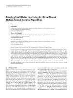
FIGURE 26-1
Probability of target detection. Figures (a) and (b) shows histograms of target and nontarget groups with respect

to some parameter value. From these histograms, the probability distribution functions of the two groups can be
estimated, as shown in (c). Using only this information, the curve in (d) can be calculated, giving the probability
that a target has been found, based on a specific value of the parameter.
Parameter value
0 5 10 15 20 25 30
0.00
0.04
0.08
0.12
0.16
0.20
non-
target
target
c. pdfs
probability of being target pdf
Number of occurencesNumber of occurences
the presence of a target, since yes will result in one action and no will result
in another. This is done by comparing the output value of the test to a
threshold. If the output is above the threshold, the test is said to be positive,
indicating that the target is present. If the output is below the threshold, the
test is said to be negative, indicating that the target is not present. In our
cancer example, a negative test result means that the patient is told they are
healthy, and sent home. When the test result is positive, additional tests will
be performed, such as obtaining a sample of the tissue by insertion of a biopsy
needle.
Since the target and nontarget distributions overlap, some test results will
not be correct. That is, some patients sent home will actually have cancer,
and some patients sent for additional tests will be healthy. In the jargon of
target detection, a correct classification is called true, while an incorrect

classification is called false. For example, if a patient has cancer, and the
test properly detects the condition, it is said to be a true-positive.
Likewise, if a patient does not have cancer, and the test indicates that
The Scientist and Engineer's Guide to Digital Signal Processing454
cancer is not present, it is said to be a true-negative. A false-positive
occurs when the patient does not have cancer, but the test erroneously
indicates that they do. This results in needless worry, and the pain and
expense of additional tests. An even worse scenario occurs with the false-
negative, where cancer is present, but the test indicates the patient is
healthy. As we all know, untreated cancer can cause many health problems,
including premature death.
The human suffering resulting from these two types of errors makes the
threshold selection a delicate balancing act. How many false-positives can
be tolerated to reduce the number of false-negatives? Figure 26-2 shows
a graphical way of evaluating this problem, the ROC curve (short for
Receiver Operating Characteristic). The ROC curve plots the percent of
target signals reported as positive (higher is better), against the percent of
nontarget signals erroneously reported as positive (lower is better), for
various values of the threshold. In other words, each point on the ROC
curve represents one possible tradeoff of true-positive and false-positive
performance.
Figures (a) through (d) show four settings of the threshold in our cancer
detection example. For instance, look at (b) where the threshold is set at 17.
Remember, every test that produces an output value greater than the threshold
is reported as a positive result. About 13% of the area of the nontarget
distribution is greater than the threshold (i.e., to the right of the threshold). Of
all the patients that do not have cancer, 87% will be reported as negative (i.e.,
a true-negative), while 13% will be reported as positive (i.e., a false-positive).
In comparison, about 80% of the area of the target distribution is greater than
the threshold. This means that 80% of those that have cancer will generate a

positive test result (i.e., a true-positive). The other 20% that have cancer will
be incorrectly reported as a negative (i.e., a false-negative). As shown in the
ROC curve in (b), this threshold results in a point on the curve at: %
nontargets positive = 13%, and % targets positive = 80%.
The more efficient the detection process, the more the ROC curve will bend
toward the upper-left corner of the graph. Pure guessing results in a straight
line at a 45E diagonal. Setting the threshold relatively low, as shown in (a),
results in nearly all the target signals being detected. This comes at the price
of many false alarms (false-positives). As illustrated in (d), setting the
threshold relatively high provides the reverse situation: few false alarms, but
many missed targets.
These analysis techniques are useful in understanding the consequences of
threshold selection, but the final decision is based on what some human will
accept. Suppose you initially set the threshold of the cancer detection
apparatus to some value you feel is appropriate. After many patients have
been screened with the system, you speak with a dozen or so patients that
have been subjected to false-positives. Hearing how your system has
unnecessarily disrupted the lives of these people affects you deeply,
motivating you to increase the threshold. Eventually you encounter a
Chapter 26- Neural Networks (and more!) 455
Parameter value
0 5 10 15 20 25 30
0.00
0.04
0.08
0.12
0.16
0.20
threshold
target

target
non-
Parameter value
0 5 10 15 20 25 30
0.00
0.04
0.08
0.12
0.16
0.20
threshold
target
target
non-
Parameter value
0 5 10 15 20 25 30
0.00
0.04
0.08
0.12
0.16
0.20
threshold
target
target
non-
Parameter value
0 5 10 15 20 25 30
0.00
0.04

0.08
0.12
0.16
0.20
threshold
target
target
non-
Threshold on pdf Point on ROC
a.
b.
c.
d.
% nontargets positive
0 20 40 60 80 100
0
20
40
60
80
100
worse
better
% nontargets positive
0 20 40 60 80 100
0
20
40
60
80

100
% nontargets positive
0 20 40 60 80 100
0
20
40
60
80
100
% nontargets positive
0 20 40 60 80 100
0
20
40
60
80
100
positivenegative
guessing
pdf
FIGURE 26-2
Relationship between ROC curves and pdfs.
% targets positive
pdf
% targets positive
pdf
% targets positive % targets positive
pdf
The Scientist and Engineer's Guide to Digital Signal Processing456
parameter 2

pdf
target
nontarget
FIGURE 26-3
Example of a two-parameter space. The
target (Î) and nontarget (~) groups are
completely separate in two-dimensions;
however, they overlap in each individual
parameter. This overlap is shown by the
one-dimensional pdfs along each of the
parameter axes.
parameter 1
situation that makes you feel even worse: you speak with a patient who is
terminally ill with a cancer that your system failed to detect. You respond to
this difficult experience by greatly lowering the threshold. As time goes on
and these events are repeated many times, the threshold gradually moves to an
equilibrium value. That is, the false-positive rate multiplied by a significance
factor (lowering the threshold) is balanced by the false-negative rate multiplied
by another significance factor (raising the threshold).
This analysis can be extended to devices that provide more than one output.
For example, suppose that a cancer detection system operates by taking an x-
ray image of the subject, followed by automated image analysis algorithms to
identify tumors. The algorithms identify suspicious regions, and then measure
key characteristics to aid in the evaluation. For instance, suppose we measure
the diameter of the suspect region (parameter 1) and its brightness in the image
(parameter 2). Further suppose that our research indicates that tumors are
generally larger and brighter than normal tissue. As a first try, we could go
through the previously presented ROC analysis for each parameter, and find an
acceptable threshold for each. We could then classify a test as positive only
if it met both criteria: parameter 1 greater than some threshold and parameter

2 greater than another threshold.
This technique of thresholding the parameters separately and then invoking
logic functions (AND, OR, etc.) is very common. Nevertheless, it is very
inefficient, and much better methods are available. Figure 26-3 shows why
this is the case. In this figure, each triangle represents a single occurrence of
a target (a patient with cancer), plotted at a location that corresponds to the
value of its two parameters. Likewise, each square represents a single
occurrence of a nontarget (a patient without cancer). As shown in the pdf
Chapter 26- Neural Networks (and more!) 457
target
nontarget
parameter 2
parameter 3
FIGURE 26-4
Example of a three-parameter space.
Just as a two-parameter space forms a
plane surface, a three parameter space
can be graphically represented using
the conventional x, y, and z axes.
Separation of a three-parameter space
into regions requires a dividing plane,
or a curved surface.
parameter 3
graph on the side of each axis, both parameters have a large overlap between
the target and nontarget distributions. In other words, each parameter, taken
individually, is a poor predictor of cancer. Combining the two parameters with
simple logic functions would only provide a small improvement. This is
especially interesting since the two parameters contain information to perfectly
separate the targets from the nontargets. This is done by drawing a diagonal
line between the two groups, as shown in the figure.

In the jargon of the field, this type of coordinate system is called a
parameter space. For example, the two-dimensional plane in this example
could be called a diameter-brightness space. The idea is that targets will
occupy one region of the parameter space, while nontargets will occupy
another. Separation between the two regions may be as simple as a straight
line, or as complicated as closed regions with irregular borders. Figure 26-
4 shows the next level of complexity, a three-parameter space being
represented on the x, y and z axes. For example, this might correspond to
a cancer detection system that measures diameter, brightness, and some
third parameter, say, edge sharpness. Just as in the two-dimensional case,
the important idea is that the members of the target and nontarget groups
will (hopefully) occupy different regions of the space, allowing the two to
be separated. In three dimensions, regions are separated by planes and
curved surfaces. The term hyperspace (over, above, or beyond normal
space) is often used to describe parameter spaces with more than three
dimensions. Mathematically, hyperspaces are no different from one, two
and three-dimensional spaces; however, they have the practical problem of
not being able to be displayed in a graphical form in our three-dimensional
universe.

The threshold selected for a single parameter problem cannot (usually) be
classified as right or wrong. This is because each threshold value results in
a unique combination of false-positives and false-negatives, i.e., some point
along the ROC curve. This is trading one goal for another, and has no
absolutely correct answer. On the other hand, parameter spaces with two or
The Scientist and Engineer's Guide to Digital Signal Processing458
more parameters can definitely have wrong divisions between regions. For
instance, imagine increasing the number of data points in Fig. 26-3, revealing
a small overlap between the target and nontarget groups. It would be possible
to move the threshold line between the groups to trade the number of false-

positives against the number of false-negatives. That is, the diagonal line
would be moved toward the top-right, or the bottom-left. However, it would be
wrong to rotate the line, because it would increase both types of errors.
As suggested by these examples, the conventional approach to target
detection (sometimes called pattern recognition) is a two step process. The
first step is called feature extraction. This uses algorithms to reduce the
raw data to a few parameters, such as diameter, brightness, edge sharpness,
etc. These parameters are often called features or classifiers. Feature
extraction is needed to reduce the amount of data. For example, a medical
x-ray image may contain more than a million pixels. The goal of feature
extraction is to distill the information into a more concentrated and
manageable form. This type of algorithm development is more of an art
than a science. It takes a great deal of experience and skill to look at a
problem and say: "These are the classifiers that best capture the
information." Trial-and-error plays a significant role.
In the second step, an evaluation is made of the classifiers to determine if
the target is present or not. In other words, some method is used to divide
the parameter space into a region that corresponds to the targets, and a
region that corresponds to the nontargets. This is quite straightforward for
one and two-parameter spaces; the known data points are plotted on a graph
(such as Fig. 26-3), and the regions separated by eye. The division is then
written into a computer program as an equation, or some other way of
defining one region from another. In principle, this same technique can be
applied to a three-dimensional parameter space. The problem is, three-
dimensional graphs are very difficult for humans to understand and
visualize (such as Fig. 26-4). Caution: Don't try this in hyperspace; your
brain will explode!
In short, we need a machine that can carry out a multi-parameter space
division, according to examples of target and nontarget signals. This ideal
target detection system is remarkably close to the main topic of this chapter, the

neural network.
Neural Network Architecture
Humans and other animals process information with neural networks. These
are formed from trillions of neurons (nerve cells) exchanging brief electrical
pulses called action potentials. Computer algorithms that mimic these
biological structures are formally called artificial neural networks to
distinguish them from the squishy things inside of animals. However, most
scientists and engineers are not this formal and use the term neural network to
include both biological and nonbiological systems.
Chapter 26- Neural Networks (and more!) 459
input layer
hidden layer
output layer
(passive nodes)
(active nodes)
(active nodes)
X1
2
X1
1
X1
3
X1
4
X1
5
X1
6
X1
7

X1
8
X1
9
X1
10
X1
11
X1
12
X1
13
X1
14
X1
15
X2
1
X2
2
X2
3
X2
4
X3
1
X3
2
Information Flow
FIGURE 26-5

Neural network architecture. This is the
most common structure for neural
networks: three layers with full inter-
connection. The input layer nodes are
passive, doing nothing but relaying the
values from their single input to their
multiple outputs. In comparison, the
nodes of the hidden and output layers
are active, modifying the signals in
accordance with Fig. 26-6. The action
of this neural network is determined by
the weights applied in the hidden and
output nodes.
Neural network research is motivated by two desires: to obtain a better
understanding of the human brain, and to develop computers that can deal with
abstract and poorly defined problems. For example, conventional computers
have trouble understanding speech and recognizing people's faces. In
comparison, humans do extremely well at these tasks.
Many different neural network structures have been tried, some based on
imitating what a biologist sees under the microscope, some based on a more
mathematical analysis of the problem. The most commonly used structure is
shown in Fig. 26-5. This neural network is formed in three layers, called the
input layer, hidden layer, and output layer. Each layer consists of one or
more nodes, represented in this diagram by the small circles. The lines
between the nodes indicate the flow of information from one node to the next.
In this particular type of neural network, the information flows only from the
input to the output (that is, from left-to-right). Other types of neural networks
have more intricate connections, such as feedback paths.
The nodes of the input layer are passive, meaning they do not modify the
data. They receive a single value on their input, and duplicate the value to

The Scientist and Engineer's Guide to Digital Signal Processing460
their multiple outputs. In comparison, the nodes of the hidden and output layer
are active. This means they modify the data as shown in Fig. 26-6. The
variables: hold the data to be evaluated (see Fig. 26-5). ForX1
1
, X1
2
þ X1
15
example, they may be pixel values from an image, samples from an audio
signal, stock market prices on successive days, etc. They may also be the
output of some other algorithm, such as the classifiers in our cancer detection
example: diameter, brightness, edge sharpness, etc.
Each value from the input layer is duplicated and sent to all of the hidden
nodes. This is called a fully interconnected structure. As shown in Fig. 26-
6, the values entering a hidden node are multiplied by weights, a set of
predetermined numbers stored in the program. The weighted inputs are then
added to produce a single number. This is shown in the diagram by the
symbol, E. Before leaving the node, this number is passed through a nonlinear
mathematical function called a sigmoid. This is an "s" shaped curve that limits
the node's output. That is, the input to the sigmoid is a value between
, while its output can only be between 0 and 1. &4 and %4
The outputs from the hidden layer are represented in the flow diagram (Fig 26-
5) by the variables: . Just as before, each of these valuesX2
1
, X2
2
, X2
3
and X2

4
is duplicated and applied to the next layer. The active nodes of the output
layer combine and modify the data to produce the two output values of this
network, and .X3
1
X3
2
Neural networks can have any number of layers, and any number of nodes per
layer. Most applications use the three layer structure with a maximum of a few
hundred input nodes. The hidden layer is usually about 10% the size of the
input layer. In the case of target detection, the output layer only needs a single
node. The output of this node is thresholded to provide a positive or negative
indication of the target's presence or absence in the input data.
Table 26-1 is a program to carry out the flow diagram of Fig. 26-5. The key
point is that this architecture is very simple and very generalized. This same
flow diagram can be used for many problems, regardless of their particular
quirks. The ability of the neural network to provide useful data manipulation
lies in the proper selection of the weights. This is a dramatic departure from
conventional information processing where solutions are described in step-by-
step procedures.
As an example, imagine a neural network for recognizing objects in a sonar
signal. Suppose that 1000 samples from the signal are stored in a computer.
How does the computer determine if these data represent a submarine,
whale, undersea mountain, or nothing at all? Conventional DSP would
approach this problem with mathematics and algorithms, such as correlation
and frequency spectrum analysis. With a neural network, the 1000 samples
are simply fed into the input layer, resulting in values popping from the
output layer. By selecting the proper weights, the output can be configured
to report a wide range of information. For instance, there might be outputs
for: submarine (yes/no), whale (yes/no), undersea mountain (yes/no), etc.

Chapter 26- Neural Networks (and more!) 461
E
x
1
x
2
x
3
x
4
x
5
x
6
x
7
SUM
SIGMOID
WEIGHT
w
1
w
3
w
2
w
4
w
5
w

6
w
7
FIGURE 26-6
Neural network active node. This is a
flow diagram of the active nodes used in
the hidden and output layers of the neural
network. Each input is multiplied by a
weight (the w
N
values), and then summed.
This produces a single value that is passed
through an "s" shaped nonlinear function
called a sigmoid. The sigmoid function is
shown in more detail in Fig. 26-7.
100 'NEURAL NETWORK (FOR THE FLOW DIAGRAM IN FIG. 26-5)
110 '
120 DIM X1[15] 'holds the input values
130 DIM X2[4] 'holds the values exiting the hidden layer
140 DIM X3[2] 'holds the values exiting the output layer
150 DIM WH[4,15] 'holds the hidden layer weights
160 DIM WO[2,4] 'holds the output layer weights
170 '
180 GOSUB XXXX 'mythical subroutine to load X1[ ] with the input data
190 GOSUB XXXX 'mythical subroutine to load the weights, WH[ , ] & W0[ , ]
200 '
210 ' 'FIND THE HIDDEN NODE VALUES, X2[ ]
220 FOR J% = 1 TO 4 'loop for each hidden layer node
230 ACC = 0 'clear the accumulator variable, ACC
240 FOR I% = 1 TO 15 'weight and sum each input node

250 ACC = ACC + X1[I%] * WH[J%,I%]
260 NEXT I%
270 X2[J%] = 1 / (1 + EXP(-ACC) ) 'pass summed value through the sigmoid
280 NEXT J%
290 '
300 ' 'FIND THE OUTPUT NODE VALUES, X3[ ]
310 FOR J% = 1 TO 2 'loop for each output layer node
320 ACC = 0 'clear the accumulator variable, ACC
330 FOR I% = 1 TO 4 'weight and sum each hidden node
340 ACC = ACC + X2[I%] * WO[J%,I%]
350 NEXT I%
360 X3[J%] = 1 / (1 + EXP(-ACC) ) 'pass summed value through the sigmoid
370 NEXT J%
380 '
390 END
TABLE 26-1
With other weights, the outputs might classify the objects as: metal or non-
metal, biological or nonbiological, enemy or ally, etc. No algorithms, no
rules, no procedures; only a relationship between the input and output dictated
by the values of the weights selected.
The Scientist and Engineer's Guide to Digital Signal Processing462
x
-7 -6 -5 -4 -3 -2 -1 0 1 2 3 4 5 6 7
0.0
0.2
0.4
0.6
0.8
1.0
a. Sigmoid function

x
-7 -6 -5 -4 -3 -2 -1 0 1 2 3 4 5 6 7
0.0
0.1
0.2
0.3
b. First derivative
s`(x)
s(x)
FIGURE 26-7
The sigmoid function and its derivative. Equations 26-1 and 26-2 generate these curves.
EQUATION 26-1
The sigmoid function. This is used in
neural networks as a smooth threshold.
This function is graphed in Fig. 26-7a.
s (x) '
1
1%e
&x
EQUATION 26-2
First derivative of the sigmoid function.
This is calculated by using the value of
the sigmoid function itself.
s N(x) ' s (x) [1 & s (x) ]
Figure 26-7a shows a closer look at the sigmoid function, mathematically
described by the equation:
The exact shape of the sigmoid is not important, only that it is a smooth
threshold. For comparison, a simple threshold produces a value of one
when , and a value of zero when . The sigmoid performs this samex > 0 x < 0
basic thresholding function, but is also differentiable, as shown in Fig. 26-7b.

While the derivative is not used in the flow diagram (Fig. 25-5), it is a critical
part of finding the proper weights to use. More about this shortly. An
advantage of the sigmoid is that there is a shortcut to calculating the value of
its derivative:
For example, if , then (by Eq. 26-1), and the first derivativex ' 0 s(x) ' 0.5
is calculated: . This isn't a critical concept, just as N(x) ' 0.5(1 & 0.5) ' 0.25
trick to make the algebra shorter.
Wouldn't the neural network be more flexible if the sigmoid could be adjusted
left-or-right, making it centered on some other value than ? The answer
x ' 0
is yes, and most neural networks allow for this. It is very simple to implement;
an additional node is added to the input layer, with its input always having a