Fundamentals of Polymer Engineering Part 10 docx
Bạn đang xem bản rút gọn của tài liệu. Xem và tải ngay bản đầy đủ của tài liệu tại đây (458.28 KB, 33 trang )
9
Thermodynamics of Polymer
Mixtures
9.1 INTRODUCTION
As with low-molecular-weight substances, the solubility of a polymer (i.e., the
amount of polymer that can be dissolved in a given liquid) depends on the
temperature and pressure of the system. In addition, however, it also depends on
the molecular weight. This fact can be used to separate a polydisperse polymer
sample into narrow molecular-weight fractions in a conceptually easy, albeit
tedious, manner. It is obvious that any help that thermodynamic theory could
afford in selecting solvent and defining process conditions would be quite useful
for optimizing polymer fractionation. Such polymers having a precise and known
molecular weight are needed in small quantities for research purposes. Although
today we use gel permeation chromatography for polymer fractionation, a
working knowledge of polymer solution thermodynamics is still necessary for
several important engineering applications [1].
In the form of solutions, polymers find use in paints and other coating
materials. They are also used in lubricants (such as multigrade motor oils), where
they temper the reduction in viscosity with increasing temperature. In addition,
aqueous polymer solutions are pumped into oil reservoirs for promoting tertiary
oil recovery. In these applications, the polymer may witness a range of
temperatures, pressures, and shear rates, and this variation can induce phase
separation. Such a situation is to be avoided, and it can be, with the aid of
374
Copyright © 2003 Marcel Dekker, Inc.
thermodynamics. Other situations in which such theory may be usefully applied
are devolatilization of polymers and product separation in polymerization
reactors. There are also instances in which we want no polymer–solvent
interactions at all, especially in cases where certain liquids come into regular
contact with polymeric surfaces.
In addition, polymer thermodynamics is very important in the growing and
commercially important area of selecting components for polymer–polymer
blends. There are several reasons for blending polymers:
1. Because new polymers with desired properties are not synthesized on a
routine basis, blending offers the opportunity to develop improved
materials that might even show a degree of synergism. For engineering
applications, it is generally desirable to develop easily processible
polymers that are dimensionally stable, can be used at high tempera-
tures, and resist attack by solvents or by the environment.
2. By varying the composition of a blend, the engineer hopes to obtain a
gradation in properties that might be tailored for specific applications.
This is true for miscible polymer pairs such as polyphenylene oxide
and polystyrene that appear and behave as single-component polymers.
3. If one of the components is a commodity polymer, its use can reduce
the cost or, equivalently, improve the profit margin for the more
expensive blended product.
Although it is possible to blend two polymers by either melt-mixing in an
extruder or dissolving in a common solvent and removing the solvent, the
procedure does not ensure that the two polymers will mix on a microscopic
level. In fact, most polymer blends are immiscible or incompatible. This means
that the mixture does not behave as a single-phase material. It will, for example,
have two different glass transition temperatures, which are representative of the
two constituents, rather than a single T
g
. Such incompatible blends can be
homogenized somewhat by using copolymers and graft polymers or by adding
surface-active agents. These measures can lead to materials having high impact
strength and toughness.
In this chapter, we presen t the classical Flory–Huggins theory, which can
explain a large number of observations regarding the phase behavior of concen-
trated polymer solutions. The agreement between theory and experiment is,
however, not always quantitative. Additionally, the theory cannot explain the
phenomenon of phase separation brought about by an increase in temperature. It
is also not very useful for describing polymer–polymer miscibility. For these
reasons, the Flory–Huggins theory has been modified and alternate theories have
been advanced, which are also discussed.
Thermodynamics of Polymer Mixtures 375
Copyright © 2003 Marcel Dekker, Inc.
9.2 CRITERIA FOR POLYMER SOLUBILITY
A polymer dissolves in a solvent if, at constant temperature and pressure, the
total Gibbs free energy can be decreased by the polymer going into solution.
Therefore, it is necessary that the following hold:
DG
M
¼ DH
mix
À T DS
mix
< 0 ð9:2:1Þ
For most polymers, the enthalpy change on mixing is positive. This necessitates
that the change in entropy be sufficiently positive if mixing is to occur. These
changes in enthalpy and entropy can be calculated using simple models; these
calculations are done in the next section. Here, we merely note that Eq. (9.2.1) is
only a necessary condition for solubility and not a sufficient condition. It is
possible, after all, to envisage an equilibrium state in which the free energy is still
lower than that corresponding to a single-phase homogeneous solution. The
single-phase solution may, for example, separate into two liquid phases having
different compositions. To understand which situation might prevail, we need to
review some elements of the thermodynamics of mixtures.
A partial molar quantity is the derivative of an extensive quantity M with
respect to the number of moles n
i
of one of the components, keeping the
temperature, the pressure, and the number of moles of all the other components
fixed. Thus,
MM
i
¼
@M
@n
i
T;P;n
j
ð9:2:2Þ
It is easy to show [2] that the mixture property M can be represented in
terms of the partial molar quantities as follows:
M ¼
P
i
MM
i
n
i
ð9:2:3Þ
For an open system at constant temperature and pressure, however,
dM ¼
P
i
MM
i
dn
i
ð9:2:4Þ
but Eq. (9.2.3) gives
dM ¼
P
i
MM
i
dn
i
þ
P
i
n
i
d
MM
i
ð9:2:5Þ
so that
P
i
n
i
d
MM
i
¼ 0 ð9:2:6Þ
which is known as the Gibbs–Duhem equation.
376 Chapter 9
Copyright © 2003 Marcel Dekker, Inc.
Let us identify M with the Gibbs free energy G and consider the mixing of
n
1
moles of pure component 1 with n
2
moles of pure component 2. Before
mixing, the free energy of both components taken together, G
comp
,is
G
comp
¼
P
2
i¼1
g
i
n
i
ð9:2:7Þ
where g
i
is the molar free energy of component i. After mixing, the free energy of
the mixture, using Eq. (9.2.3), is as follows:
G
mixture
¼
P
2
i¼1
GG
i
n
i
ð9:2:8Þ
Consequently, the change in free energy on mixing is
DG
M
¼
P
2
i¼1
ð
GG
i
À g
i
Þn
i
ð9:2:9Þ
and dividing both sides by the total number of moles, n
1
þ n
2
,yieldsthe
corresponding result for 1 mol of mixture,
Dg
m
¼
P
2
i¼1
ð
GG
i
À g
i
Þx
i
ð9:2:10Þ
where x
i
denotes mole fraction.
It is common practice to call the partial molar Gibbs free energy
GG
i
the
chemical potential and write it as m
i
. Clearly, g
i
is the partial molar Gibbs free
energy for the pure component. Representing it as m
0
i
, we can derive from
Eq. (9.2.10) the following:
Dg
m
¼ x
1
Dm
1
þ x
2
Dm
2
ð9:2:11Þ
where Dm
1
¼ m
1
À m
0
1
and Dm
2
¼ m
2
À m
0
2
. Because x
1
þ x
2
equals unity,
Eq. (9.2.11) can be written
Dg
m
¼ Dm
1
þ x
2
ðDm
2
À Dm
1
Þð9:2:12Þ
Differentiating this result with respect to x
2
gives
dDg
m
dx
2
¼
dm
1
dx
2
þðDm
2
À Dm
1
Þþx
2
dm
2
dx
2
À
dm
1
dx
2
ð9:2:13Þ
¼ðDm
2
À Dm
1
Þþx
2
dm
2
dx
2
þ x
1
dm
1
dx
2
From Eq. (9.2.6), however,
P
2
1
x
i
dm
i
equals 0. Therefore, Eq. (9.2.13) becomes
dDg
m
dx
2
¼ Dm
2
À Dm
1
ð9:2:14Þ
Thermodynamics of Polymer Mixtures 377
Copyright © 2003 Marcel Dekker, Inc.
and solving Eq. (9.2.14) simultaneously with Eq. (9.2.11) yields
Dm
1
¼ Dg
m
À x
2
dDg
m
dx
2
ð9:2:15Þ
Dm
2
¼ Dg
m
þ x
1
dDg
m
dx
2
ð9:2:16Þ
Thus, if Dg
m
can be obtained by some means as a function of composition, the
chemical potentials can be computed using Eqs. (9.2.15) and (9.2.16). The
chemical potentials are, in turn, needed for phase equilibrium calculations.
Let us now return to the question of whether a single-phase solution or two
liquid phases will be formed if the DG
M
of a two-component system is negative.
This question can be answered by examining Figure 9.1, which shows two
possible Dg
m
versus x
2
curves; these two curves may correspond to different
temperatures. It can be reasoned from Eqs. (9.2.15) and (9.2.16) that the chemical
potentials at any composition x
2
can be determined simply by drawing a tangent to
the Dg
m
curve at x
2
and extending it until it intersects with the x
2
¼ 0 and x
2
¼ 1
axes. The intercept with x
2
¼ 0 gives Dm
1
, whereas that with x
2
¼ 1givesDm
2
.
Following this reasoning, it is seen that the curve labeled T
1
has a one-to-
one correspondence between Dm
1
and x
2
or, for that matter, between Dm
2
and x
2
.
This happens because the entire curve is concave upward. Thus, there are no two
composition values that yield the same value of the chemical potential. This
implies that equilibrium is not possible between two liquid phases of differing
compositions; instead, there is complete miscibility. At a lower temperature T
2
,
however, the chemical potential at x
0
2
equals the chemical potential at x
00
2
.
Solutions of these two compositions can, therefore, coexist in equilibrium. The
points x
0
2
and x
00
2
are called binodal points, and any single-phase system having a
composition between these two points can split into these two phases with relative
FIGURE 9.1 Free-energy change of mixing per mole of a binary mixture as a function
of mixture composition.
378 Chapter 9
Copyright © 2003 Marcel Dekker, Inc.
amountsofeachphasedeterminedbyamassbalance.Phaseseparationoccurs
becausethefreeenergyofthetwo-phasemixturedenotedbythepointmarkedDg
islessthanthefreeenergyDg*ofthesingle-phasesolutionofthesameaverage
composition.PointsS
0
andS
00
areinflectionpointscalledspinodalpoints,and
betweenthesetwopointstheDg
m
curveisconcavedownward.Asolutionhaving
acompositionbetweenthesetwopointsisunstabletoeventhesmallest
disturbanceandcanloweritsfreeenergybyphaseseparation.Betweeneach
spinodalpointandthecorrespondingbinodalpoint,however,Dg
m
isconcave
upwardand,therefore,stabletosmalldisturbances.Thisiscalledametastable
region;here,itispossibletoobserveasingle-phasesolution—butonlyfora
limitedperiodoftime.
Thepresenceofthetwo-phaseregiondependsontemperature.Forsome
solutions,atahighenoughtemperaturecalledtheuppercriticalsolution
temperature,thespinodalandbinodalpointscometogetherandonlysingle-
phasemixturesoccurabovethistemperature.ThissituationisdepictedinFigure
9.2onatemperature–compositiondiagram.Here,thelocusofthebinodalpoints
iscalledthebinodalcurveorthecloudpointcurve,whereasthelocusofthe
spinodalpointsiscalledthespinodalcurve.Next,wedirectourattentionto
determiningthefree-energychangeonmixingapolymerwithalow-molecular-
weightsolvent.
9.3THEFLORY^HUGGINSTHEORY
TheclassicalFlory–Hugginstheoryassumesattheoutsetthatthereisneithera
changeinvolumenorachangeinenthalpyonmixingapolymerwithalow-
molecular-weightsolvent[3–5];theinfluenceofnon-athermal(DH
mixing
6¼0)
behaviorisaccountedforatalaterstage.Thus,thecalculationofthefree-energy
FIGURE9.2Temperature–compositiondiagramcorrespondingtoFigure9.1.
Thermodynamics of Polymer Mixtures 379
Copyright © 2003 Marcel Dekker, Inc.
change on mixing at a constant temperature and pressure reduces to a calculation
of the change in entropy on mixing. This latter quantity is determined with the
help of a lattice model using formulas from statistical thermodynamics.
We assume the existence of a two-dimensional lattice with each lattice site
having z nearest neighbors, where z is the coordination number of the lattice; an
example is shown in Figure 9.3. Each lattice site can accommodate a single
solvent molecule or a polymer segment having a volume equal to a solvent
molecule. Polymer molecules are taken to be monodisperse, flexible, initially
disordered, and composed of a series of segments the size of a solvent molecule.
The number of segments in each polymer molecule is m, which equals V
2
=V
1
,the
ratio of the molar volume of the polymer to the molar volume of the solvent. Note
that m is not the degree of polymerization.
We begin with an empty lattice and calculate the number of ways, O,of
arranging n
1
solvent molecules and n
2
polymer molecules in the n
0
¼ n
1
þ mn
2
lattice sites. Because the heat of mixing has been taken to be zero, each
arrangement has the same energy and is equally likely to occur. The only
restriction imposed is by the connectivity of polymer chain segments. It must
be ensured that two segments connected to each other lie on the nearest
neighboring lattice sites. Once O is known, the entropy of the mixture is given
by k ln O; where k is Boltzmann’s constant.
9.3.1 Entropy Change on Mixing
In order to calculate the entropy of the mixture, we first arrange all of the polymer
molecules on the lattice. The identical solvent molecules are placed thereafter. If j
FIGURE 9.3 Schematic diagram of a polymer molecule on a two-dimensional lattice.
380 Chapter 9
Copyright © 2003 Marcel Dekker, Inc.
polymer molecules have already been placed, the number of lattice sites still
available number n
0
À jm. Thus, the first segment of the ð j þ 1Þst molecule can
be arranged in n
0
À jm ways. The second segment is connected to the first one
and so can be placed only in one of the z neighboring sites. All of these may,
however, not be vacant. If the polymer solution is relatively concentrated so that
chain overlap occurs, we would expect that, on average, the fraction of
neighboring sites occupied ð f Þ would equal the overall fraction of sites occupied.
Thus, f ¼ jm=n
0
. As a result, the second segment of the ð j þ 1Þst molecule can
be placed in zð1 Àf Þ ways. Clearly, the third segment can be placed in
ðz À 1 Þð1 À f Þ ways, and similarly for subseq uent segments. Therefore, the
total number of ways O
jþ1
in which the ð j þ 1Þst polymer molecule can be
arranged is the product of the number of ways of placing the first segment with
the number of ways of placing the second segment and the number of ways of
placing each subsequent segment. Thus,
O
jþ1
¼ðn
0
À jmÞzð1 Àf Þ
Q
m
3
ðz À 1Þð1 À f Þð9:3:1Þ
where the symbol
Q
denotes product. As a consequence,
O
jþ1
¼ðn
0
À jmÞzðz À1Þ
mÀ2
ð1 À f Þ
mÀ1
ffiðn
0
À jmÞðz À1Þ
mÀ1
ð1 À f Þ
mÀ1
¼ðn
0
À jmÞðz À1Þ
mÀ1
1 À
jm
n
0
mÀ1
¼ðn
0
À jmÞ
m
z À 1
n
0
mÀ1
ð9:3:2Þ
The total number of ways of arranging all of the n
2
polymer molecules, O
p
,isthe
product of the number of ways of arranging each of the n
2
molecules in sequence.
This fact and Eq. (9.3.2) yield
O
p
¼
Q
n
2
À1
j¼0
ðn
0
À jmÞ
m
z À 1
n
0
mÀ1
"#
ð9:3:3Þ
where the index only goes up to n
2
À 1 because j ¼ 0 corresponds to the first
polymer molecule. The development so far assumes that all of the polymer
molecules are different. They are, however, identical to each other. This reduces
the total number of possible arrangements by a factor of n
2
!, and it is therefore
necessary to divide the right-hand side of Eq. (9.3.3) by n
2
!.
Having arranged all of the polymer molecules, the number of ways of
fitting all of the indistinguishable solvent molecules into the remaining lattice
Thermodynamics of Polymer Mixtures 381
Copyright © 2003 Marcel Dekker, Inc.
sites is exactly one. As a result, O
p
equals O, the total number of ways of placing
all the polymer and solvent molecules on to the lattice. Finally, then,
S
mixture
¼ k ln O ð9:3:4Þ
and using Eq. (9.3.3) properly divided by n
2
!:
S
mixture
k
¼Àlnðn
2
!Þþm
P
n
2
À1
j¼0
lnðn
0
À jmÞþðm À 1 Þ
P
n
2
À1
j¼0
ln
z À 1
n
0
ð9:3:5Þ
Because j does not appear in the last term on the right-hand side of Eq. (9.3.5),
that term adds up to ðm À 1Þn
2
ln½ðz À 1Þ=n
0
. Also, the first term can be replaced
by Stirling’s approximation:
ðn
2
!Þ¼n
2
ln n
2
À n
2
ð9:3:6Þ
Now, consider the summation in the second term:
P
n
2
À1
j¼0
lnðn
0
À jmÞ¼
P
n
2
À1
j¼0
ln
m
n
0
m
À j
¼ n
2
ln m þ
P
n
2
À1
j¼0
ln
n
0
m
À j
ð9:3:7Þ
Furthermore,
P
n
2
À1
j¼0
ln
n
0
m
À j
¼ ln
n
0
m
þ ln
n
0
m
À 1
þÁÁÁþln
n
0
m
À n
2
þ 1
¼ ln
n
0
m
n
0
m
À 1
n
0
m
À 2
ÁÁÁ
n
0
m
À n
2
þ 1
hi
¼ ln
n
0
m
n
0
m
À 1
ÁÁÁ
n
0
m
À n
2
þ 1
n
0
m
À n
2
ÁÁÁ1
n
0
m
À n
2
ÁÁÁ1
8
>
<
>
:
9
>
=
>
;
¼ ln
ðn
0
=mÞ!
ðn
0
=m À n
2
Þ!
ð9:3:8Þ
382 Chapter 9
Copyright © 2003 Marcel Dekker, Inc.
Combining all of these fragments and again using Stirling’s approximation in
Eq. (9.3.8) yields
S
mixture
k
¼Àn
2
ln n
2
þ n
2
þ m
n
2
ln m þ
n
0
m
ln
n
0
m
À
n
0
m
À
n
0
m
À n
2
ln
n
0
m
À n
2
þ
n
0
m
À n
2
þðm À 1 Þn
2
ln
z À 1
n
0
ð9:3:9Þ
which, without additional tricks, can be simplified to the following:
S
mixture
k
¼Àn
2
ln
n
2
n
0
þ n
2
À mn
2
À n
1
ln
n
1
n
0
ð9:3:10Þ
þðm À 1 Þ½n
2
lnðz À 1Þ
Adding to and subtracting n
2
ln m from the right-hand side of Eq. (9.3.10) gives
the result
S
mixture
k
¼Àn
2
ln
mn
2
n
0
À n
1
ln
n
1
n
0
þ n
2
½ðm À 1Þlnðz À 1Þþð1 ÀmÞþln m ð9:3:11Þ
The entropy of the pure polymer S
2
can be obtained by letting n
1
be zero and n
0
be mn
2
in Eq. (9.3.11):
S
2
k
¼ n
2
½ðm À 1Þlnðz À 1Þþð1 À mÞþln mð9:3:12Þ
Similarly, the entropy of the pure solvent S
1
is obtained by setting n
2
equal to zero
and n
1
equal to n
0
:
S
1
k
¼ 0 ð9:3:13Þ
Using Eqs. (9.3.11)–(9.3.13),
DS
mixing
¼ DS
mixture
À S
1
À S
2
¼Àkn
1
ln
n
1
n
0
þ n
2
ln
mn
2
n
0
ð9:3:14Þ
From the way that m and n
0
have been defined, it is evident that n
1
=n
0
equals f
1
,
the volume fraction of the solvent, and mn
2
=n
0
equals f
2
, the volume fraction of
the polymer. As a result,
DS ¼Àk½n
1
ln f
1
þ n
2
ln f
2
ð9:3:15Þ
Thermodynamics of Polymer Mixtures 383
Copyright © 2003 Marcel Dekker, Inc.
which is independent of the lattice coordination number z. The change in entropy
on mixing n
1
moles of solvent with n
2
moles of polymer will exceed by a factor
of Avogadro’s number the change in entropy given by Eq. (9.3.15); multiplying
the right-hand side of this equation by Avogadro’s number gives
DS ¼ÀR½n
1
ln f
1
þ n
2
ln f
2
ð9:3:16Þ
where R is the universal gas constant and n
1
and n
2
now represent numbers of
moles. Note that if m were to equal unity, f
1
and f
2
would equal the mole
fractions and Eq. (9.3.16) would become identical to the equation for the change
in entropy of mixing ideal molecules [2]. Note also that Eq. (9.3.16) does not
apply to dilute solutions because of the assumption that f equals jm=n
0
and is
independent of position within the lattice.
Example 9.1: One gram of polymer having molecular weight 40,000 and density
1g=cm
3
is dissolved in 9 g of solvent of molecular weight 78 and density
0.9 g=cm
3
.
(a) What is the entropy change on mixing?
(b) How would the answer change if a monomer of molecular weight 100
were dissolved in place of the polymer?
Solution:
(a) n
1
¼ 9=78 ¼ 0:115; n
2
¼ 2:5 Â10
À5
; f
1
¼ð9=0:9Þ=½ð9=0:9Þþ1¼
0:909; f
2
¼ 0:091. Therefore, DS ¼ÀR½0:115 ln 0:909 þ 2:5Â
10
À5
ln 0:091¼0:011R.
(b) In this case, DS ¼ÀR½n
1
ln x
1
þ n
2
ln x
2
, with n
2
¼ 0:01; x
1
¼ 0:92,
and x
2
¼ 0:08 so that DS ¼ 0:035R.
9.3.2 Enthalpy Change on Mixing
If polymer solutions were truly athermal, DG of mixing would equal ÀTDS, and,
based on Eq. (9.3.16), this would always be a negative quantity. The fact that
polymers do not dissolve very easily suggests that mixing is an endothermic
process and DH > 0. If the change in volume on mixing is again taken to be zero,
DH equals DU , the internal energy change on mixing. This latter change arises
due to interactions between polymer and solvent molecules. Because intermole-
cular forces drop off rapidly with increasing distance, we need to consider only
nearest neighbors in evaluating DU. Consequently, we can again use the lattice
model employed previously.
Let us examine the filled lattice and pick a polymer segment at random. It is
surrounded by z neighbors. Of these, zf
2
are polymeric and zf
1
are solvent. If the
384 Chapter 9
Copyright © 2003 Marcel Dekker, Inc.
energy of interaction (a negative quantity) between two polymer segments is
represented by e
22
and that between a polymer segment and a solvent molecule by
e
12
, the total energy of interaction for the single polymer segment is
zf
2
e
22
þ zf
1
e
12
Because the total number of polymer segments in the lattice is n
0
f
2
,the
interaction energy associated with all of the polymer segments is
z
2
n
0
f
2
ðf
2
e
22
þ f
1
e
12
Þ
where the factor of
1
2
has been added to prevent everything from being counted
twice.
Again, by similar reasoning, the total energy of interaction for a single
solvent molecule picked at random is
zf
1
e
11
þ zf
2
e
12
where e
11
is the energy of interaction between two solvent molecules. Because
the total number of solvent molecules is n
0
f
1
, the total interaction energy is
zn
0
f
1
2
ðf
1
e
11
þ f
2
e
12
Þ
For the pure polymer, the energy of interaction between like segments before
mixing (using a similar lattice) is
n
0
f
2
ze
22
2
For pure solvent, the corresponding quantity is
n
0
f
1
ze
11
2
From all of these equations, the change in energy on mixing, DU,isthe
difference between the sum of the interaction energy associated with the polymer
and solvent in solution and the sum of the interaction energy of the pure
components. Thus,
DU ¼
z
2
n
0
f
2
ðf
2
e
22
þ f
1
e
12
Þþ
zn
0
f
1
2
ðf
1
e
11
þ f
2
e
12
Þ
À
n
0
f
2
ze
22
2
À
n
0
f
1
ze
11
2
¼
zn
0
2
½2f
1
f
2
e
12
À f
1
f
2
e
11
À f
1
f
2
e
22
¼ Dezn
0
f
1
f
2
ð9:3:17Þ
Thermodynamics of Polymer Mixtures 385
Copyright © 2003 Marcel Dekker, Inc.
where De ¼ð1=2Þð2e
12
À e
11
À e
22
Þ, and the result is found to depend on the
unknown coordination number z. Because z is not known, it makes sense to lump
De along with it and define a new unknown quantity w
1
, called the interaction
parameter:
w
1
¼
zDe
kT
ð9:3:18Þ
whose value is zero only for athermal mixtures. For endothermic mixing, w
1
is
positive (the more common situation), whereas for exothermic mixing, it is
negative. Combining Eqs. (9.3.17) and (9.3.18) yields
DH
M
¼ DU
M
¼ kT w
1
n
0
f
1
f
2
ð9:3:19Þ
¼ kT w
1
n
1
f
2
and the magnitude of w
1
has to be estimated by comparison with experimental
data.
9.3.3 Free-Energy Change and Chemical
Potentials
If we assume that the presence of a nonzero DH
M
does not influence the
previously calculated DS
M
, a combination of Eqs. (9.2.1), (9.3.15 ), and
(9.3.19) yields
DG
M
¼ kT ½n
1
ln f
1
þ n
2
ln f
2
þ w
1
n
1
f
2
ð9:3:20Þ
Because volume fractions are always less than unity, the first two terms in
brackets in Eq. (9.3.20) are negative. The third term depends on the sign of the
interaction parameter, but it is usually positive. From Eq. (9.3.18), however, w
1
decreases with increasing temperature so that DG
M
should always become
negative at a sufficiently high temperature. It is for this reason that a polymer–
solvent mixture is warmed to promote solubility. Also note that if one increases
the polymer molecular weight while keeping n
1
; f
1
; f
2
, and T constant, n
2
decreases because the volume per polymer molecule increases. The consequence
of this fact, from Eq. (9.3.20), is that DG
M
becomes less negative, which implies
that a high-molecular-weight fraction is less likely to be soluble than a low-
molecular-weight fraction. This also means that if a saturated polymer solution
containing a polydisperse sample is cooled, the highest-molecular-weight compo-
nent will precipitate first. In order to quantify these statements, we have to use the
thermodynamic phase equilibrium criterion [2]
m
A
i
¼ m
B
i
ð9:3:21Þ
386 Chapter 9
Copyright © 2003 Marcel Dekker, Inc.
where i ¼ 1; 2 and A and B are the two phases that are in equilibrium. In writing
Eq. (9.3.21), it is assumed that the polymer, component 2, is monodisperse. The
effect of polydispersity will be discussed later.
The chemical potentials required in Eq. (9.3.21) can be computed using
Eq. (9.3.20), the definition of the chemical potential as a partial molar Gibbs
free energy, and the fact that
DG
M
¼ G
mixture
À G
1
À G
2
ð9:3:22Þ
so that
G
mixture
¼ n
1
g
1
þ n
2
g
2
þ RT ½n
1
ln f
1
þ n
2
ln f
2
þ w
1
n
1
f
2
ð9:3:23Þ
where n
1
and n
2
now denote numbers of moles rather than numbers of molecules,
and g
1
and g
2
are the molar free energies of the solvent and polymer, respectively.
Differentiating Eq. (9.3.23) with respect to n
1
and n
2
, in turn, gives the following:
m
1
¼
@G
mixture
@n
1
¼ g
1
þ RT ln f
1
þ
n
1
f
1
@f
1
@n
1
þ
n
2
f
2
@f
2
@n
1
þ w
1
f
2
þ w
1
n
1
@f
2
@n
1
ð9:3:24Þ
m
2
¼
@G
mixture
@n
2
¼ g
2
þ RT
n
1
f
1
@f
1
@n
2
þ ln f
2
þ
n
2
f
2
@f
2
@n
2
þ w
1
n
1
@f
2
@n
2
ð9:3:25Þ
Recognizing that
f
1
¼
n
1
n
1
þ mn
2
and f
2
¼
mn
2
n
1
þ mn
2
gives the following:
@f
1
@n
1
¼
f
2
n
1
þ mn
2
ð9:3:26Þ
@f
1
@n
2
¼À
mf
1
n
1
þ mn
2
ð9:3:27Þ
@f
2
@n
1
¼À
f
2
n
1
þ mn
2
ð9:3:28Þ
@f
2
@n
2
¼
mf
1
n
1
þ mn
2
ð9:3:29Þ
Thermodynamics of Polymer Mixtures 387
Copyright © 2003 Marcel Dekker, Inc.
IntroducingtheseresultsintoEqs.(9.3.24)and(9.3.25)andsimplifyinggives
m
1
Àm
0
1
RT
¼lnð1Àf
2
Þþf
2
1À
1
m
þw
1
f
2
2
ð9:3:30Þ
m
2
Àm
0
2
RT
¼ð1Àf
2
Þð1ÀmÞþlnf
2
þw
1
mð1Àf
2
Þ
2
ð9:3:31Þ
inwhichg
1
andg
2
havebeenrelabeledm
0
1
andm
0
2
,respectively.Thepreceding
twoequationscannowbeusedforexaminingphaseequilibrium.
9.3.4PhaseBehaviorofMonodisperse
Polymers
Ifwemixn
1
molesofsolventwithn
2
molesofpolymerhavingaknownmolar
volumeormolecularweight(i.e.,aknownvalueofm),thechemicalpotentialof
thesolventinsolutionisgivenbyEq.(9.3.30).Ifwefixw
1
,wecaneasilyplot
ðm
1
Àm
0
1
Þ=RTasafunctionoff
2
.Bychangingw
1
andrepeatingtheprocedure,
wegetafamilyofcurvesatdifferenttemperatures,becausethereisaone-to-one
correspondencebetweenw
1
andtemperature.SuchaplotisshowninFigure9.4
formequaling1000,takenfromtheworkofFlory[3,5].Notethatincreasingw
1
isequivalenttodecreasingtemperature.
ByexaminingFigure9.4,wefindthatforvaluesofw
1
belowacriticalvalue
w
c
,thereisauniquerelationshipbetweenm
1
andf
2
.Abovew
c
,however,theplots
arebivalued.Becausethesamevalueofthechemicalpotentialoccursattwo
differentvaluesoff
2
,thesetwovaluesoff
2
cancoexistatequilibrium.Inother
words,twophasesareformedwheneverw
1
>w
c
.Tocalculatethevalueofw
c
,
notethatatw
1
¼w
c
,thereisaninflectionpointinthem
1
versusf
2
curve.Thus,
wecanobtainw
c
bysettingthefirsttwoderivativesofm
1
withrespecttof
2
equal
tozero.UsingEq.(9.3.30)tocarryoutthesedifferentiations,
@m
1
@f
2
¼À
1
1Àf
2
þ1À
1
m
þ2w
1
f
2
ð9:3:32Þ
@
2
m
1
@f
2
2
¼À
1
ð1Àf
2
Þ
2
þ2w
1
ð9:3:33Þ
Atw
1
¼w
c
andf
2
¼f
2c
;thesetwoderivativesarezero.Solvingforw
c
from
eachofthetwoequationsyieldsthefollowing:
w
c
¼
1
2f
2c
ð1Àf
2c
Þ
À1À
1
m
ð2f
2c
Þ
À1
ð9:3:34Þ
w
c
¼
1
2ð1Àf
2c
Þ
2
ð9:3:35Þ
388Chapter9
Copyright © 2003 Marcel Dekker, Inc.
Equatingtheright-handsidesofthetwopreviousequationsgives
f
2c
¼
1
1þ
ffiffiffiffi
m
p
ð9:3:36Þ
whichmeansthat
w
c
¼
1
2
þ
1
ffiffiffiffi
m
p
þ
1
2m
ð9:3:37Þ
andw
c
!
1
2
asmbecomesverylarge.Thus,knowingmallowsustoderivew
c
or,
equivalently,thetemperatureatwhichtwoliquidphasesfirstbegintoappear;this
istheuppercriticalsolutiontemperature(UCST)showninFigure9.2.The
correspondingUCSTforpolymerofinfinitemolecularweightisknownasthe
Florytemperatureorthetatemperature,anditishigherthantheUCSTofpolymer
havingafinitemolecularweight.Itisclear,however,thatifthetheoryisvalid,
completesolubilityshouldbeobservedforw
1
0:5.Itisalsodesirabletoplotthe
binodalorthetemperature–compositioncurveseparatingtheone-andtwo-phase
FIGURE9.4Solventchemicalpotentialasafunctionofpolymervolumefractionfor
m ¼ 1000. The value of w
1
is indicated on each curve. (Reprinted from Paul J. Flory,
Principles of Polymer Chemistry. Copyright #1953 Cornell University and copyright #
1981 Paul J. Flory. Used by permission of the Publisher, Cornell University Press.)
Thermodynamics of Polymer Mixtures 389
Copyright © 2003 Marcel Dekker, Inc.
regions. The procedure for doing this is deferred until after we discuss the method
of numerically relating w
1
to temperature.
9.3.5 Determining the Interaction Parameter
The polymer–solvent interaction parameter w
1
can be calculated from Eq. (9.3.30)
in conjunction with any experimental technique that allows for a measurement of
the chemical potential. This can be done via any one of several methods,
including light scattering and viscosity, but most commonly with the help of
vapor-pressure or osmotic pressure measurements [1–6]. Let us examine both.
If we consider a pure vapor to be ideal, then the following is true at constant
temperature:
dm ¼ dg ¼ v dP ¼
RT
P
dP ð9:3:38Þ
where g and v are the molar free energy and molar volume, respectively.
Integrating from a pressure P
0
to pressure P gives
mðT; PÞÀmðT; P
0
Þ¼RT ln
P
P
0
ð9:3:39Þ
The equivalent expression for a component, say 1, in a mixture of ideal gases
with mole fraction y
1
is given by the following [2]:
m
1
ðT; P; y
1
ÞÀm
1
ðT; P
0
Þ¼RT ln
Py
1
P
0
ð9:3:40Þ
If the vapor is in equilibrium with a liquid phase, the chemical potential of each
component has to be the same in both phases. Also, for a pure liquid at
equilibrium, P equals the vapor pressure P
0
1
. Thus, denoting as m
0
1
the pure
liquid 1 chemical potential, we can derive the following, using Eq. (9.3.39):
m
0
1
¼ m
1
ðT; P
0
ÞþRT ln
P
0
1
P
0
ð9:3:41Þ
Similarly, for component 1 in a liquid mixture in equilibrium with a mixture of
gases, the liquid-phase chemical potential is, from Eq. (9.3.40),
m
1
¼ m
1
ðT; P
0
ÞþRT ln
Py
1
P
0
ð9:3:42Þ
Subtracting Eq. (9.3.41) from Eq. (9.3.42) to eliminate m
1
ðT; P
0
Þ gives the
following [7]:
m
1
À m
0
1
¼ RT ln
Py
1
P
0
1
ð9:3:43Þ
390 Chapter 9
Copyright © 2003 Marcel Dekker, Inc.
butPy
1
isthepartialpressureP
1
ofcomponent1inthegasphase.Combining
Eqs.(9.3.30)and(9.3.43)gives
ln
P
1
P
0
1
¼lnð1Àf
2
Þþf
2
1À
1
m
þw
1
f
2
2
ð9:3:44Þ
wheretheleft-handsideisalsowrittenasa
1
,inwhicha
1
isthesolventactivity.
Thus,measurementsofP
1
asafunctionoff
2
canbeusedtoobtainw
1
overa
widerangeofconcentrations.
ThesituationwithosmoticequilibriumisshownschematicallyinFigure
8.4,andithasbeendiscussedpreviouslyinChapter8.Atequilibrium,the
chemicalpotentialofthesolventisthesameonbothsidesofthesemipermeable
membrane.Thus,
m
1
ðT;PÞ¼m
1
ðT;Pþp;x
1
Þð9:3:45Þ
wherepistheosmoticpressureandx
1
isthemolefractionofsolventinsolution.
Fromelementarythermodynamics,however,
m
1
ðT;Pþp;x
1
Þ¼m
1
ðT;P;x
1
Þþ
ð
Pþp
P
VV
1
dPð9:3:46Þ
inwhich
VV
1
isthepartialmolarvolume.Thetermm
1
ðT;PÞisthesameaswhat
wehavebeencallingm
0
1
;therefore,Eqs.(9.3.45)and(9.3.46)implythat
m
1
Àm
0
1
¼À
ð
Pþp
P
VV
1
dPffiÀv
1
dpð9:3:47Þ
becausethepartialmolarvolumeisnottoodifferentfromthemolarvolumeof
thesolvent.
UsingtheFlory–Hugginsexpressionforthedifferenceinchemicalpoten-
tialsinEq.(9.3.47)gives
p¼À
RT
v
1
lnð1Àf
2
Þþ1À
1
m
f
2
þw
1
f
2
2
ð9:3:48Þ
whichcanberewritteninaslightlydifferentformifweexpand1Àf
2
inaTaylor
seriesaboutf
2
¼0.Retainingtermsuptof
3
2
,weget
p¼
RT
v
1
f
2
m
þ
1
2
Àw
1
f
2
2
þ
f
3
2
3
þÁÁÁ
"#
ð9:3:49Þ
whichcanagainbeusedtoevaluatew
1
usingexperimentaldata.Acomparisonof
Eq.(9.3.49)withEq.(8.3.22)showsthatthesecondvirialcoefficientis0atthe
thetatemperaturebecausew
1
equals0.5atthatcondition.
Typicaldataforw
1
asafunctionoff
2
obtainedusingthesemethodsare
showninFigure9.5[5].Itisfoundthatalthoughsolutionsofrubberinbenzene
Thermodynamics of Polymer Mixtures 391
Copyright © 2003 Marcel Dekker, Inc.
behave as expected, most systems are characterized by a concentration-dependent
interaction parameter [5,8]. In addition, w
1
does not follow the expected inverse
temperature dependence predicted by theory [5]. This suggests that DH
M
is not
independent of temperature. To take the temperature dependence of DH
M
into
account, Flory uses the following expression for w
1
that involves two new
constants, y and c [5]:
w
1
¼
1
2
À c 1 À
y
T
ð9:3:50Þ
One way of determining these constants is to first determine the upper critical
solution temperature, T
c
, as a function of polymer molecular weight. At T
c
, w
1
is
equal to w
c
. Equations (9.3.37) and (9.3.50) therefore yield
1
2
þ
1
ffiffiffiffi
m
p
þ
1
2m
¼
1
2
À c 1 À
y
T
c
ð9:3:51Þ
or, upon rearrangement,
1
T
c
¼
1
y
1 þ
1
c
1
2m
þ
1
ffiffiffiffi
m
p
ð9:3:52Þ
FIGURE 9.5 Influence of composition on the polymer–solvent interaction parameter.
Experimental values of the interaction parameter w
1
are plotted against the volume fraction
f
2
of polymer. Data for polydimethylsiloxane (M ¼ 3850) in benzene (n), polystyrene in
methyl ethyl ketone (d), and polystyrene in toluene (s) are based on vapor-pressure
measurements. Those for rubber in benzene (.) were obtained using vapor-pressure
measurements at higher concentrations and isothermal distillation equilibration with
solutions of known activities in the dilute range. (Reprinted from Paul J. Flory, Principles
of Polymer Chemistry. Copyright # 1953 Cornell University and copyright # 1981 Paul
J. Flory. Used by permission of the Publisher, Cornell University Press.)
392 Chapter 9
Copyright © 2003 Marcel Dekker, Inc.
sothataplotof1=T
c
versus½ð1=2mÞþð1=
ffiffiffiffi
m
p
Þshouldbeastraightlinewitha
slopeof1=ycandaninterceptof1=y.Theseare,infact,theresultsobtainedby
SchultzandFlory[9],andthisallowsforeasydeterminationofcandy.Clearly,
w
1
equals0.5whenTequalsyand,therefore,theparameteryisthetheta
temperaturereferredtoearlierandisthemaximuminthecloudpointcurveforan
infinite-molecular-weightpolymer.Itcanbeshownthatatthethetatemperature,
theeffectofattractionbetweenpolymersegmentsexactlycancelstheeffectofthe
excludedvolumeandtherandomcoildescribedinthenextchapterexactlyobeys
Gaussianstatistics.Also,theMark–Houwinkexponentequals
1
2
undertheta
conditions.
Thevalueoftheinteractionparameterisoftenusedasameasureofsolvent
quality.Solventsarenormallydesignatedas‘‘good’’ifw
1
<0:5and‘‘poor’’if
w
1
>0:5;aninteractionparametervalueofexactly0.5denotesanidealsolventor
athetasolvent.
Example9.2:ListedinTable9.1aredatafortheuppercriticalsolution
temperatureofsixpolystyrene(PS)-in-dioctylphthalate(DOP)solutionsasa
functionofmolecularweight[10].Alsogivenisthecorrespondingratioofmolar
volumes.Determinethetemperaturedependenceoftheinteractionparameter.
Solution:ThedataofTable9.1areplottedinFigure9.6accordingto
Eq.(9.3.52).Fromthestraight-linegraph,wefindthatc¼1:45and
y¼288K.Thisvalueofthethetatemperatureisbracketedbysimilarvalues
estimatedbyviscometryandlight-scatteringtechniques[10].
9.3.6CalculatingtheBinodal
OncetheinteractionparameterintheformofEq.(9.3.50)hasbeendetermined,
theentiretemperature–compositionphasediagramorthebinodalcurvecanbe
calculatedusingtheconditionsofphaseequilibrium.Atachosentemperature,let
thetwopolymercompositionsinequilibriumwitheachotherbef
C
2
andf
D
2
.Let
TABLE9.1UCSTDataforSolutionsofPSinDOP
Molecular weight (Â10
À5
) UCST (
C) Molar volume ratio (Â10
À3
)
2.00 5.9 0.456
2.80 7.4 0.639
3.35 8.0 0.770
4.70 8.8 1.072
9.00 9.9 2.069
18.00 12.0 4.131
Source: Ref. 10.
Thermodynamics of Polymer Mixtures 393
Copyright © 2003 Marcel Dekker, Inc.
thecorrespondingchemicalpotentialsbem
C
2
andm
D
2
.Becausethelattertwo
valuesmustbeequaltoeachother,Eq.(9.3.31)impliesthefollowing:
lnf
C
2
ÀðmÀ1Þð1Àf
C
2
Þþw
1
mð1Àf
C
2
Þ
2
¼lnf
D
2
ÀðmÀ1Þð1Àf
D
2
Þþw
1
mð1Àf
D
2
Þ
2
ð9:3:53Þ
Thisequationcanbesolvedtogivew
1
intermsoff
C
2
andf
D
2
.Anotherexpression
forw
1
intermsoff
C
2
andf
D
2
canbeobtainedbyusingEq.(9.3.30)toequatethe
chemicalpotentialsofthesolventinthetwophases.Thesetwoexpressionsforw
1
canbeusedtoobtainasingleequationrelatingf
C
2
tof
D
2
.Thereafter,wesimply
pickavalueoff
C
2
andsolveforthecorrespondingvalueoff
D
2
.Bypicking
enoughdifferentvaluesoff
C
2
,wecantracetheentirebinodalcurvebecausethe
valueofw
1
and,therefore,Tisknownforanyorderedpairf
C
2
;f
D
2
.Approximate
analyticalexpressionsfortheresultingcompositionsandtemperaturehavebeen
providedbyFlory[5],andsampleresultsforthepolyisobutylene-in-diisobutyl
ketonesystemareshowninFigure9.7[5,9].Althoughthetheoreticalpredictions
arequalitativelycorrect,thecriticalpointoccursatalowerthanmeasured
concentration.Also,thecalculatedbinodalregionistoonarrow.Tompahas
shownthatmuchmorequantitativeagreementcouldbeobtainedifw
1
weremade
toincreaselinearlywithpolymervolumefraction[11].Weshall,however,not
pursuethisaspectofthetheoryhere.
Inclosingthissubsection,wenotethatthephaseequilibriumcalculation
forpolydispersepolymersisconceptuallystraightforwardbutmathematically
tedious.Eachpolymerfractionhastobetreatedasaseparatespecieswithitsown
chemicalpotentialgivenbyanequationsimilartoEq.(9.3.31).Theinteraction
parameter,however,istakentobeindependentofmolecularweight.Itis
FIGURE9.6Plotofthereciprocalofthecriticalprecipitationtemperatures(1=T
c
)
against½1=
ffiffiffiffi
m
p
þ1=ð2mÞforsixpolystyrenefractionsinDOP.(FromRef.10.)
394Chapter9
Copyright © 2003 Marcel Dekker, Inc.
necessary to again equate chemical potentials in the two liquid phases and carry
out proper mass balances to obtain enough equations in all of the unknowns.
Details are available elsewhere [12]. The procedure can be used to predict the
results of polymer fractionation [13].
9.3.7 Strengths and Weaknesses of the
Flory^Huggins Model
The Flory–Huggins theory, which has been described in detail in this chapter, is
remarkably successful in explaining most observations concerning the phase
behavior of polymer–solvent systems. For a binary mixture, this theory includes
the prediction of two liquid phases and the shift of the critical point to lower
concentrations as the molecular weight is increased (see Fig. 9.7). In addition, the
theory can explain the phase behavior of a three-component system—whether it
is two polymers dissolved in a common solvent or a single polymer dissolved in
two solvents. The former situation is relevant to polymer blending [14], whereas
the latter is important in the formation of synthetic fibers [15] and membranes
[16] by phase inversion due to the addition of nonsolvent. Computation of the
phase diagram is straightforward [5], and results are represented on triangular
FIGURE 9.7 Phase diagram for three polyisobutylene fractions (molecular weights
indicated) in diisobutyl ketone. Solid curves are drawn through the experimental points.
The dashed curves have been calculated from theory. (Reprinted with permission from
Shultz, A. R., and P. J. Flory: ‘‘Phase Equilibria in Polymer-Solvent Systems,’’ J. Am.
Chem. Soc., vol. 74, pp. 4760–4767, 1952. Copyright 1952 American Chemical Society.)
Thermodynamics of Polymer Mixtures 395
Copyright © 2003 Marcel Dekker, Inc.
diagrams.Note,though,thattheindexiinEq.(9.3.21)rangesfrom1to3and,in
general,wehavethreeseparateinteractionparametersrelatingthethreedifferent
components.Wemayalsousethetheorytointerprettheswellingequilibriumof
cross-linkedpolymersbroughtintocontactwithgoodsolvents[5].Becausea
cross-linkedpolymercannotdissolve,itimbibessolventinamannersimilarto
thatinosmosis.Aswithosmosis,theprocessisagainself-limitingbecause
swellingcausespolymercoilexpansion,generatingaretractileforce(seeChapter
10)thatcounteractsfurtherabsorptionofthesolvent.Theextentofswellingcan
beusedtoestimatethevalueofthepolymer–solventinteractionparameter.A
technologicalapplicationofthisphenomenonisinthesynthesisofporous
polymersorbentsasreplacementsforactivatedcarbonusedintheremovalof
volatileorganiccompoundsfromwastewaterstreams.Inthisprocess,anonpor-
ouspolymerislightlycross-linkedandthenmadetoswellwiththehelpofan
appropriatesolvent[17].Furthercross-linkingintheswollenstategivesa
materialhavingaveryhighdegreeofporosity.
TheFlory–Hugginstheoryhasweaknesses,however.Althoughsome
quantitativedisagreementbetweentheobservedandpredictedsizeofthebinodal
regionhasalreadybeennoted,themajorfailurehastodowiththeinabilityto
predictphaseseparationaboveacriticaltemperature,knownasthelowercritical
solutiontemperature.FreemanandRowlinsonhavefoundthatevennonpolar
polymersthatdonotinteractwiththesolventwoulddemixwithincreasing
temperature[18].BecausetheDSofmixingisalwayspositiveintheFlory–
Hugginstheoryandbecausew
1
alwaysdecreaseswithincreasingtemperature,
suchaphaseseparationistotallyinexplicable.Theresolutionofthisenigmais
discussedinthenextsection.WeclosethissectionbyalsonotingthattheFlory–
Hugginstheoryfailsforverydilutesolutionsduetothebreakdownofthe
spatiallyuniformpolymerconcentrationassumption.Theactualentropychange
onmixingisfoundtobelessthanthepredictedtheoreticalvaluebecausepolymer
moleculesindilutesolutionexistasisolatedrandomcoilswhosesizesarea
functionofthemolecularweight.Thismakesw
1
afunctionofthepolymerchain
length[5,19].
NotethattheFlory–Hugginstheoryappliestoflexiblemacromolecules
only.Rodlikeparticlescanbetreatedinananalogousmanner[20]andtheresults
canbeusedtoexplainthebehaviorofpolymericliquidcrystals.
9.4FREE-VOLUMETHEORIES
AbasicassumptionintheFlory–Hugginstheoryistheabsenceofachangein
volumeonmixing.This,however,isnotexactlytrue.AsPattersonexplainsinhis
veryreadablereview[21],thefreevolumeofthepolymerdiffersmarkedlyfrom
thesolventfreevolume.(SeeChapter13foranextensivediscussionaboutthe
396 Chapter 9
Copyright © 2003 Marcel Dekker, Inc.
free volume.) The solvent is much more ‘‘expanded’’due to its larger free volume.
When mixing occurs, the solvent loses its free volume and there is a net decrease
in the total volume. This result is analogous to, but not the same as, the process of
condensation of a gas; in a condensation process, latent heat is evolved and there
is an increase in order. Thus, both DH and DS are negative. This happens even
when the polymer and the solvent are chemically similar. Both of these
contributions need to be included in the free-energy change on mixing. As the
free-volume dissimilarity between the polymer and the solvent increases with
increasing temperature, the free-volume effect is likely to be more important at
elevated temperatures. One way of accounting for this effect is to consider the
interaction parameter w
1
to be composed of an entropic part in addition to the
enthalpic part. Thus,
w
1
¼ w
H
þ w
S
ð9:4:1Þ
Indeed, Eq. (9.3.50) already does this, with w
H
being cy=T and w
S
being ð
1
2
À cÞ.
Now, we also have to add the free-volume contributions. This is done using an
equation of state that allows for a calculation of the volume, enthalpy, and entropy
change on mixing from a knowledge of the pure-component properties and a
limited amount of solution data. Qualitatively, though, we expect the w
1
contribution arising from free-volume effects to increase with increasing tempera-
ture. This is shown in Figure 9.8. When this free-volume contribution is added to
the interaction parameter given by Eq. (9.3.50), the result is a minimum in the w
1
versus temperature curve. Because phase separation originates from a large
FIGURE 9.8 (a) Phase diagram of a polymer solution showing the phase separation
occurring at high temperatures above the lower critical solution temperature (LCST). (b)
The temperature dependence of the w
1
parameter: curve 3, total w
1
; curve 2, contribution to
w
1
due to free-volume dissimilarity between polymer and solvent; curve 1, contribution to
w
1
due to contact-energy dissimilarity between polymer and solvent. (Reprinted with
permission from Patterson, D.: ‘‘Free volume and Polymer Solubility: A Qualitative View,’’
Macromolecules, vol. 2, pp. 672–677, 1969. Copyright 1969 American Chemical Society.)
Thermodynamics of Polymer Mixtures 397
Copyright © 2003 Marcel Dekker, Inc.
positivevalueofw
1
andbecausethiscannowhappenatbothlowandhigh
temperatures,thephenomenonofalowercriticalsolutiontemperatureiseasily
understood.Notethatthecriticalvalueofw
1
isstillgivenbyEq.(9.3.37),but,as
seenfromFigure9.8,itnowcorrespondstotwodifferenttemperatures—alower
criticalsolutiontemperatureandanuppercriticalsolutiontemperature.Except
forthischange,thephaseboundariesareagaincomputedusingtheprocedure
outlinedinSection9.3.6.Adescriptionoftheactualprocedureforcomputingthe
modifiedw
1
versustemperaturecurveshownschematicallyinFigure9.8is
beyondthescopeofthisbook,butdetailsareavailableintheliterature[22–24].
Notethatusingthefree-volumetheorypermitsustoexplaintheexistenceofan
interactionparameterthatdependsonbothtemperatureandconcentrationina
mannerthatlogicallyleadstothepredictionofalowercriticalsolution
temperature.
9.5THESOLUBILITYPARAMETER
ThesolubilityparameterofHildebrand[25],generallydenotedd,isauseful
alternativetotheinteractionparameterw
1
inmanysituations.Itisusedtoestimate
theendothermicheatofmixingthataccompaniesthedissolutionofanamor-
phouspolymerbyalow-molecular-weightsolvent.Thetechniquehasbeenused
extensivelyinthepaintandrubberindustries[26].Intheformerapplication,the
parameterisusedforidentifyingappropriatesolvents,andinthelatter,itisused
forpreventingtheswellingofvolcanizedrubberbysolvents.Aswillbeseen
here, the major argument in favor of using the solubility parameter is that solution
properties are not required; all necessary information can be obtained from data
on pure components.
For purposes of motivation, let us consider the mixing of n
1
molecules of a
low-molecular-weight species with n
2
molecules of another low-molecular-
weight species having the same volume v per molecule. Then, using the same
argument enunciated in Section 9.3.2 [setting m as unity in Eq. (9.3.17)], the
following can be derived:
DH
M
¼ znf
1
f
2
½e
12
À
1
2
ðe
11
þ e
22
Þ ð9:5:1Þ
in which n equals n
1
þ n
2
and the e
ij
terms are all negative quantities. Denoting
Avogadro’s number by N
A
and the total mixture volume by V, Eq. (9.5.1) can be
rewritten as
DH
M
¼
V f
1
f
2
N
A
v
ÀN
A
z je
12
jþ
N
A
2
z je
11
jþ
N
A
z
2
je
22
j
ð9:5:2Þ
in which v is the volume per molecule. To make further progress, we assume that
je
12
j¼
ffiffiffiffiffiffiffiffiffiffiffiffiffiffiffiffiffi
je
11
jje
22
j
p
ð9:5:3Þ
398 Chapter 9
Copyright © 2003 Marcel Dekker, Inc.