2001 Fundamentals Part 1 ppsx
Bạn đang xem bản rút gọn của tài liệu. Xem và tải ngay bản đầy đủ của tài liệu tại đây (610.91 KB, 15 trang )
CONTRIBUTORS
In addition to the Technical Committees, the following individuals contributed significantly
to this volume. The appropriate chapter numbers follow each contributor’s name.
Charles H. Bemisderfer (1)
York International
Donald C. Erickson (1)
Energy Concepts Co.
Hans-Martin Hellmann (1)
Zent-Frenger
Thomas H. Kuehn (1, 6)
University of Minnesota
Christopher P. Serpente (1)
Carrier Corp.
Robert M. Tozer (1)
Waterman-Gore M&E Consulting
Engineers
Anthony M. Jacobi (2)
University of Illinois at Urbana-
Champaign
Dr. Arthur E. Bergles (3)
Rensselaer Polytechnic Institute
Michael M. Ohadi (3, 5)
University of Maryland
Steven J. Eckels (4)
Kansas State University
Rick J. Couvillion (5)
University of Arkansas
Albert C. Kent (5)
Southern Illinois University
Ray Rite (5)
Trane Company
Jason T. LeRoy (6)
Trane Company
Warren E. Blazier, Jr. (7)
Warren Blazier Associates, Inc.
Alfred C. C. Warnock (7)
National Research Council Canada
Larry G. Berglund (8)
U.S. Army Research Institute for
Environmental Medicine
Gemma Kerr (9, 12)
InAir Environmental Ltd.
D.J. Marsick (9)
U.S. Department of Energy
D.J. Moschandreas (9)
The Institute for Science, Law, and
Technology
Kenneth M. Wallingford (9)
NIOSH
Richard S. Gates (10)
University of Kentucky
Albert J. Heber (10)
Purdue University
Farhad Memarzadeh (10)
National Institutes of Health
Gerald L. Riskowski (10, 11)
University of Illinois
Yuanhui Zhang (10)
University of Illinois
Roger C. Brook (11)
Michigan State University
Joe F. Pedelty (12, 13)
Holcomb Environmental Services
Pamela Dalton (13)
Monell Chemical Senses Center
Martin Kendal-Reed (13)
Florida State University Sensory Research
Institute
James C. Walker (13)
Florida State University Research Institute
Rick Stonier (14)
Gray Wolf Sensing Solutions
Monica Y. Amalfitano (15)
P2S Engineering
James J. Coogan (15)
Siemens Building Technologies
David M. Underwood (15)
USA-CERL
John J. Carter (16)
CPP Inc.
Dr. David J. Wilson (16)
University of Alberta
William J. Coad (17)
McClure Engineering Assoc.
David Grumman (17)
Grumman/Butkus Associates
Douglas W. DeWerth (18)
Robert G. Doerr (19)
The Trane Company
Eric W. Lemmon (20)
National Institute of Standards and
Technology
Mark O. McLinden (20)
National Institute of Standards and
Technology
Steven G. Penoncello (20)
University of Idaho
Sherry K. Emmrich (21)
Dow Chemical
Lewis G. Harriman III (22)
Mason-Grant Company
Hugo L.S.C. Hens (23)
Katholieke Universiteit
Achilles N. Karagiozis (23)
Oak Ridge National Laboratory
Hartwig M. Kuenzel (23)
Fraunhofer Institut Bauphysik
Anton TenWolde (23)
Forest Products Laboratory
William Brown (24)
Morrison Herschfield
Andre Desjarlais (24)
Oak Ridge National Laboratory
David Roodvoets (24)
DLR Consultants
William B. Rose (24, 25)
University of Illinois
William P. Goss (25)
University of Massachusetts
Malcolm S. Orme (26)
Air Infiltration and Ventilation Centre
Andrew K. Persily (26)
National Institute of Standards and
Technology
Brian A. Rock (26)
University of Kansas
Armin F. Rudd (26)
Building Science Corporation
Max H. Sherman (26)
Lawrence Berkeley National Laboratory
Iain S. Walker (26)
Lawrence Berkeley National Laboratory
Craig P. Wray (26)
Lawrence Berkeley National Laboratory
University of Nebraska-Omaha
Grenville K. Yuill (26)
University of Nebraska-Omaha
Robert Morris (27)
Environment Canada
Climate and Water Products Division
Raymond G. Alvine (28)
Jim Norman (28)
AAA Enterprises
Charles F. Turdik (28)
Lynn Bellenger (29)
Pathfinder Engineers LLP
Steven Bruning (29)
Newcomb & Boyd
Curt Petersen (29)
Thomas Romine (29)
Romine, Romine & Burgess
Christopher Wilkins (29)
Hallam Associates
D. Charlie Curcija (30)
University of Massachusetts
William C. duPont (30)
Lawrence Berkeley National Laboratory
John F. Hogan (30)
Joseph H. Klems (30)
Lawrence Berkeley National Laboratory
W. Ross McCluney (30)
Florida Solar Energy Center
M. Susan Reilly (30)
Enermodal Engineering
Eleanor S. Lee (30)
Lawrence Berkeley National Laboratory
David Tait (30)
Tait Solar
Leslie Norford (31)
Massachusetts Institute of Technology
Fred S. Bauman (32)
University of California
Mohammad H. Hosni (32)
Kansas State University
Leon Kloostra (32)
TITUS, Division of Tomkins
Raymond H. Horstman (33)
Boeing Commercial Airplanes
Herman F. Behls (34)
Behls & Associates
Albert W. Black (35)
McClure Engineering Associates
ASHRAE HANDBOOK COMMITTEE
Dennis J. Wessel, Chair
2001 Fundamentals Volume Subcommittee: George Reeves, Chair
David E. Claridge Frederick H. Kohloss Brian A. Rock T. David Underwood Michael W. Woodford
ASHRAE HANDBOOK STAFF
Jeanne Baird, Associate Editor
Scott A. Zeh, Nancy F. Thysell, and Jayne E. Jackson, Publishing Services
W. Stephen Comstock,
Director, Communications and Publications
Publisher
ASHRAE Research: Improving the Quality of Life
The American Society of Heating, Refrigerating and Air-Condi-
tioning Engineers is the world’s foremost technical society in the
fields of heating, ventilation, air conditioning, and refrigeration. Its
members worldwide ideas, identify needs, support research, and
write the industry’s standards for testing and practice. The result is
that engineers are better able to keep indoor environments safe and
productive while protecting and preserving the outdoors for gener-
ations to come.
One of the ways that ASHRAE supports its members’ and indus-
try’s need for information is through ASHRAE Research. Thou-
sands of individuals and companies support ASHRAE Research
annually, enabling ASHRAE to report new data about material
properties and building physics and to promote the application of
innovative technologies.
The chapters in ASHRAE Handbooks are updated through the
experience of members of ASHRAE technical committees and
through results of ASHRAE Research reported at ASHRAE meet-
ings and published in ASHRAE special publications and in
ASHRAE Transactions.
For information about ASHRAE Research or to become a mem-
ber contact, ASHRAE, 1791 Tullie Circle, Atlanta, GA 30329; tele-
phone: 404-636-8400; www.ashrae.org.
The 2001 ASHRAE Handbook
The Fundamentals volume covers basic principles and provides
data for the practice of HVAC&R technology. Although design data
change little over time, research sponsored by ASHRAE and others
continues to generate new information that meets the evolving
needs of the people and industries that rely on HVAC&R technol-
ogy to improve the quality of life. The ASHRAE technical commit-
tees that prepare chapters strive to provide new information, clarify
existing information, delete obsolete materials and reorganize chap-
ters to make the Handbook more understandable and easier to use.
In this volume, some of the changes and additions are as follows:
• Chapter 1, Thermodynamics and Refrigeration Cycles, includes
new sections on ideal thermal and absorption cycles, multiple
stage cycles, and thermodynamic representation of absorption
cycles. The section on ammonia water cycles has been expanded.
• Chapter 12, Air Contaminants, has undergone major revisions.
Material has been added from the 1999 ASHRAE Handbook,
Chapter 44, Control of Gaseous Indoor Air Contaminants.
Health-related material with standards and guidelines for expo-
sure has been moved to Chapter 9, Indoor Environmental Health.
• Chapter 15, Fundamentals of Control now includes new or
revised figures on discharge air temperature control, step input
process, and pilot positioners. New are sections on networking
and fuzzy logic, revised descriptions on dampers and modulating
control, and text on chilled mirror humidity sensors and disper-
sive infrared technology.
• Chapter 17, Energy Resources, contains new sections on sustain-
ability and designing for effective energy resource use.
• Chapter 19, Refrigerants, provides information on phaseout of
CFC and HCFC refrigerants and includes new data on R-143a
and R-404A, R-407C, R-410A, R-507, R-508A, and R-508B
blends.
• Chapter 20, Thermophysical Properties of Refrigerants, has new
data on R-143a and R-245fa. Though most CFC Refrigerants
have been removed from the chapter, R-12 has been retained to
assist in making comparisons. Revised formulations have been
used for many of the HFC refrigerants, conforming to interna-
tional standards where applicable.
• Chapter 23, Thermal and Moisture Control in Insulated Assem-
blies—Fundamentals, now has a reorganized section on eco-
nomic insulation thickness, a revised surface condensation
section, and a new section on moisture analysis models.
• Chapter 26, Ventilation and Infiltration, includes rewritten stack
pressure and wind pressure sections. New residential sections dis-
cuss averaging time variant ventilation, superposition methods,
the enhanced (AIM-2) model, air leakage through automatic
doors, and central air handler blowers in ventilation systems. The
nonresidential ventilation section has also been rewritten, and
now includes a commercial building envelope leakage measure-
ments summary.
• Chapter 27, Climatic Design Information, now contains new
monthly, warm-season design values for some United States loca-
tions. These values aid in consideration of seasonal variations in
solar geometry and intensity, building occupancy, and use patterns.
• Chapter 29, Nonresidential Cooling and Heating Load Calcula-
tions, now contains enhanced data on internal loads, an expanded
description of the heat balance method, and the new, simplified
radiant time series (RTS) method.
• Chapter 30, Fenestration, now has revised solar heat gain and vis-
ible transmittance sections, including information on the solar
heat gain coefficients (SHGC) method. The chapter now also has
a rewritten section on solar-optical properties of glazings, an
expanded daylighting section, and a new section on occupant
comfort and acceptance.
• Chapter 31, Energy Estimating and Modeling Methods, now con-
tains improved model forms for both design and existing building
performance analysis. A new section describes a simplified
method for calculating heat flow through building foundations
and basements. Sections on secondary equipment and bin-energy
method calculations have added information, while the section on
data-driven models has been rewritten and now illustrates the
variable-base degree-day method.
• Chapter 32, Space Air Diffusion, has been reorganized to be more
user-friendly. The section on principles of jet behavior now
includes simpler equations with clearer tables and figures. Tem-
perature profiles now accompany characteristics of different out-
lets, with stagnant regions identified. The section on underfloor
air distribution and task/ambient conditioning includes updates
from recent ASHRAE-sponsored research projects.
• Chapter 33, HVAC Computational Fluid Dynamics, is a new
chapter that provides an introduction to computational methods in
flow modeling, including a description of computational fluid
dynamics (CFD) with discussion of theory and capabilities.
• Chapter 34, Duct Design, includes revisions to duct sealing
requirements from ASHRAE Standard 90.1, and has been
expanded to include additional common fittings, previously
included in electronic form in ASHRAE’s Duct Fitting Database.
This Handbook is published both as a bound print volume and in
electronic format on a CD-ROM. It is available in two editions—
one contains inch-pound (I-P) units of measurement, and the other
contains the International System of Units (SI).
Look for corrections to the 1998, 1999, and 2000 Handbooks on
the Internet at . Any changes in this volume
will be reported in the 2002 ASHRAE Handbook and on the
ASHRAE web site.
If you have suggestions for improving a chapter or you would
like more information on how you can help revise a chapter, e-mail
; write to Handbook Editor, ASHRAE, 1791
Tullie Circle, Atlanta, GA 30329; or fax 404-321-5478.
ASHRAE TECHNICAL COMMITTEES AND TASK GROUPS
SECTION 1.0—FUNDAMENTALS AND GENERAL
1.1 Thermodynamics and Psychrometrics
1.2 Instruments and Measurements
1.3 Heat Transfer and Fluid Flow
1.4 Control Theory and Application
1.5 Computer Applications
1.6 Terminology
1.7 Operation and Maintenance Management
1.8 Owning and Operating Costs
1.9 Electrical Systems
1.10 Energy Resources
SECTION 2.0—ENVIRONMENTAL QUALITY
2.1 Physiology and Human Environment
2.2 Plant and Animal Environment
2.3 Gaseous Air Contaminants and Gas Contaminant
Removal Equipment
2.4 Particulate Air Contaminants and Particulate
Contaminant Removal Equipment
2.6 Sound and Vibration Control
2.7 Seismic and Wind Restraint Design
TG Buildings’ Impacts on the Environment
TG Global Climate Change
SECTION 3.0—MATERIALS AND PROCESSES
3.1 Refrigerants and Secondary Coolants
3.2 Refrigerant System Chemistry
3.3 Refrigerant Contaminant Control
3.4 Lubrication
3.5 Desiccant and Sorption Technology
3.6 Water Treatment
3.8 Refrigerant Containment
SECTION 4.0—LOAD CALCULATIONS AND ENERGY
REQUIREMENTS
4.1 Load Calculation Data and Procedures
4.2 Weather Information
4.3 Ventilation Requirements and Infiltration
4.4 Building Materials and Building Envelope Performance
4.5 Fenestration
4.6 Building Operation Dynamics
4.7 Energy Calculations
4.10 Indoor Environmental Modeling
4.11 Smart Building Systems
4.12 Integrated Building Design
TG Mechanical Systems Insulation
SECTION 5.0—VENTILATION AND AIR DISTRIBUTION
5.1 Fans
5.2 Duct Design
5.3 Room Air Distribution
5.4 Industrial Process Air Cleaning (Air Pollution Control)
5.5 Air-to-Air Energy Recovery
5.6 Control of Fire and Smoke
5.7 Evaporative Cooling
5.8 Industrial Ventilation
5.9 Enclosed Vehicular Facilities
5.10 Kitchen Ventilation
SECTION 6.0—HEATING EQUIPMENT, HEATING AND
COOLING SYSTEMS AND APPLICATIONS
6.1 Hydronic and Steam Equipment and Systems
6.2 District Energy
6.3 Central Forced Air Heating and Cooling Systems
6.4 In Space Convection Heating
6.5 Radiant Space Heating and Cooling
6.6 Service Water Heating
6.7 Solar Energy Utilization
6.8 Geothermal Energy Utilization
6.9 Thermal Storage
6.10 Fuels and Combustion
SECTION 7.0—PACKAGED AIR-CONDITIONING AND
REFRIGERATION EQUIPMENT
7.1 Residential Refrigerators and Food Freezers
7.4 Combustion Engine Driven Heating and Cooling
Equipment
7.5 Mechanical Dehumidification Equipment and Heat Pipes
7.6 Unitary and Room Air Conditioners and Heat Pumps
SECTION 8.0—AIR-CONDITIONING AND
REFRIGERATION SYSTEM COMPONENTS
8.1 Positive Displacement Compressors
8.2 Centrifugal Machines
8.3 Absorption and Heat Operated Machines
8.4 Air-to-Refrigerant Heat Transfer Equipment
8.5 Liquid-to-Refrigerant Heat Exchangers
8.6 Cooling Towers and Evaporative Condensers
8.7 Humidifying Equipment
8.8 Refrigerant System Controls and Accessories
8.10 Pumps and Hydronic Piping
8.11 Electric Motors and Motor Control
SECTION 9.0—AIR-CONDITIONING SYSTEMS AND
APPLICATIONS
9.1 Large Building Air-Conditioning Systems
9.2 Industrial Air Conditioning
9.3 Transportation Air Conditioning
9.4 Applied Heat Pump/Heat Recovery Systems
9.5 Cogeneration Systems
9.6 Systems Energy Utilization
9.7 Testing and Balancing
9.8 Large Building Air-Conditioning Applications
9.9 Building Commissioning
9.10 Laboratory Systems
9.11 Clean Spaces
9.12 Tall Buildings
TG Combustion Gas Turbine Inlet Air Cooling Systems
SECTION 10.0—REFRIGERATION SYSTEMS
10.1 Custom Engineered Refrigeration Systems
10.2 Automatic Icemaking Plants and Skating Rinks
10.3 Refrigerant Piping, Controls, and Accessories
10.4 Ultra-Low Temperature Systems and Cryogenics
10.5 Refrigerated Distribution and Storage Facilities
10.6 Transport Refrigeration
10.7 Commercial Food and Beverage Cooling Display
and Storage
10.8 Refrigeration Load Calculations
10.9 Refrigeration Application for Foods and Beverages
TG Mineral Oil Circulation
1.1
CHAPTER 1
THERMODYNAMICS AND REFRIGERATION CYCLES
THERMODYNAMICS 1.1
First Law of Thermodynamics 1.2
Second Law of Thermodynamics 1.2
Thermodynamic Analysis of Refrigeration Cycles 1.3
Equations of State 1.3
Calculating Thermodynamic Properties 1.4
COMPRESSION REFRIGERATION CYCLES 1.6
Carnot Cycle 1.6
Theoretical Single-Stage Cycle Using a Pure Refrigerant
or Azeotropic Mixture 1.8
Lorenz Refrigeration Cycle 1.9
Theoretical Single-Stage Cycle Using Zeotropic
Refrigerant Mixture 1.10
Multistage Vapor Compression Refrigeration
Cycles 1.10
Actual Refrigeration Systems 1.12
ABSORPTION REFRIGERATION CYCLES 1.14
Ideal Thermal Cycle 1.14
Working Fluid Phase Change
Constraints 1.14
Working Fluids 1.15
Absorption Cycle Representations 1.16
Conceptualizing the Cycle 1.16
Absorption Cycle Modeling 1.17
Ammonia-Water Absorption Cycles 1.19
Nomenclature for Examples 1.20
HERMODYNAMICS is the study of energy, its transforma-
Ttions, and its relation to states of matter. This chapter covers the
application of thermodynamics to refrigeration cycles. The first part
reviews the first and second laws of thermodynamics and presents
methods for calculating thermodynamic properties. The second and
third parts address compression and absorption refrigeration cycles,
the two most common methods of thermal energy transfer.
THERMODYNAMICS
A thermodynamic system is a region in space or a quantity of
matter bounded by a closed surface. The surroundings include
everything external to the system, and the system is separated from
the surroundings by the system boundaries. These boundaries can
be movable or fixed, real or imaginary.
The concepts that operate in any thermodynamic system are
entropy and energy. Entropy measures the molecular disorder of a
system. The more mixed a system, the greater its entropy; con-
versely, an orderly or unmixed configuration is one of low entropy.
Energy has the capacity for producing an effect and can be catego-
rized into either stored or transient forms as described in the follow-
ing sections.
Stored Energy
Thermal (internal) energy is the energy possessed by a system
caused by the motion of the molecules and/or intermolecular forces.
Potential energy is the energy possessed by a system caused by
the attractive forces existing between molecules, or the elevation of
the system.
(1)
where
m =mass
g = local acceleration of gravity
z = elevation above horizontal reference plane
Kinetic energy is the energy possessed by a system caused by
the velocity of the molecules and is expressed as
(2)
where V is the velocity of a fluid stream crossing the system
boundary.
Chemical energy is energy possessed by the system caused by
the arrangement of atoms composing the molecules.
Nuclear (atomic) energy is energy possessed by the system
from the cohesive forces holding protons and neutrons together as
the atom’s nucleus.
Energy in Transition
Heat (Q) is the mechanism that transfers energy across the
boundary of systems with differing temperatures, always toward the
lower temperature. Heat is positive when energy is added to the sys-
tem (see Figure 1).
Work is the mechanism that transfers energy across the bound-
ary of systems with differing pressures (or force of any kind),
always toward the lower pressure. If the total effect produced in the
system can be reduced to the raising of a weight, then nothing but
work has crossed the boundary. Work is positive when energy is
removed from the system (see Figure 1).
Mechanical or shaft work (W ) is the energy delivered or
absorbed by a mechanism, such as a turbine, air compressor, or
internal combustion engine.
Flow work is energy carried into or transmitted across the sys-
tem boundary because a pumping process occurs somewhere out-
side the system, causing fluid to enter the system. It can be more
easily understood as the work done by the fluid just outside the
The preparation of the first and second parts of this chapter is assigned to
TC 1.1, Thermodynamics and Psychrometrics. The third part is assigned to
TC 8.3, Absorption and Heat-Operated Machines.
PE mgz=
KE mV
2
2⁄=
Fig. 1 Energy Flows in General Thermodynamic System
2.1
CHAPTER 2
FLUID FLOW
Fluid Properties 2.1
Basic Relations of Fluid Dynamics 2.1
Basic Flow Processes 2.3
Flow Analysis 2.7
Noise from Fluid Flow 2.13
LOWING fluids in heating, ventilating, air-conditioning, and
Frefrigeration systems transfer heat and mass. This chapter intro-
duces the basics of fluid mechanics that are related to HVAC pro-
cesses, reviews pertinent flow processes, and presents a general
discussion of single-phase fluid flow analysis.
FLUID PROPERTIES
Fluids differ from solids in their reaction to shearing. When
placed under shear stress, a solid deforms only a finite amount,
whereas a fluid deforms continuously for as long as the shear is
applied. Both liquids and gases are fluids. Although liquids and
gases differ strongly in the nature of molecular actions, their pri-
mary mechanical differences are in the degree of compressibility
and liquid formation of a free surface (interface).
Fluid motion can usually be described by one of several simpli-
fied modes of action or models. The simplest is the ideal-fluid
model, which assumes no resistance to shearing. Ideal flow analysis
is well developed (Baker 1983, Schlichting 1979, Streeter and
Wylie 1979), and when properly interpreted is valid for a wide range
of applications. Nevertheless, the effects of viscous action may need
to be considered. Most fluids in HVAC applications can be treated
as Newtonian, where the rate of deformation is directly proportional
to the shearing stress. Turbulence complicates fluid behavior, and
viscosity influences the nature of the turbulent flow.
Density
The density ρ of a fluid is its mass per unit volume. The densities
of air and water at standard indoor conditions of 20°C and 101.325
kPa (sea level atmospheric pressure) are
Viscosity
Viscosity is the resistance of adjacent fluid layers to shear. For
shearing between two parallel plates, each of area A and separated
by distance Y, the tangential force F per unit area required to slide
one plate with velocity V parallel to the other is proportional to V/Y:
where the proportionality factor µ is the absolute viscosity or
dynamic viscosity of the fluid. The ratio of the tangential force F to
area A is the shearing stress τ, and V/Y is the lateral velocity gra-
dient (Figure 1A). In complex flows, velocity and shear stress may
vary across the flow field; this is expressed by the following differ-
ential equation:
(1)
The velocity gradient associated with viscous shear for a simple
case involving flow velocity in the x direction but of varying mag-
nitude in the y direction is illustrated in Figure 1B.
Absolute viscosity µ depends primarily on temperature. For gases
(except near the critical point), viscosity increases with the square
root of the absolute temperature, as predicted by the kinetic theory.
Liquid viscosity decreases with increasing temperature. Viscosities of
various fluids are given in Chapter 38.
Absolute viscosity has dimensions of force · time/length
2
. At
standard indoor conditions, the absolute viscosities of water and dry
air are
In fluid dynamics, kinematic viscosity ν is the ratio of absolute
viscosity to density:
At standard indoor conditions, the kinematic viscosities of water
and dry air are
BASIC RELATIONS OF FLUID DYNAMICS
This section considers homogeneous, constant-property, incom-
pressible fluids and introduces fluid dynamic considerations used in
most analyses.
The preparation of this chapter is assigned to TC 1.3, Heat Transfer and
Fluid Flow.
ρ
water
998 kg m
3
⁄=
ρ
air
1.20 kg m
3
⁄=
FA⁄µVY⁄()=
Fig. 1 Velocity Profiles and Gradients in Shear Flows
τµ
dv
dy
=
µ
water
1.0 mN·s/m
2
=
µ
air
18 µN·s/m
2
=
νµρ⁄=
ν
water
1.00 10
6–
× m
2
/s=
ν
air
16 10
4–
× m
2
/s=
2.2 2001 ASHRAE Fundamentals Handbook (SI)
Continuity
Conservation of matter applied to fluid flow in a conduit requires
that
where
v = velocity normal to the differential area dA
ρ=fluid density
Both ρ and v may vary over the cross section A of the conduit. If
both ρ and v are constant over the cross-sectional area normal to the
flow, then
(2a)
where is the mass flow rate across the area normal to the flow.
When flow is effectively incompressible, ρ = constant; in pipeline
and duct flow analyses, the average velocity is then V = (1/A)
∫
vdA.
The continuity relation is
(2b)
where Q is the volumetric flow rate. Except when branches occur, Q
is the same at all sections along the conduit.
For the ideal-fluid model, flow patterns around bodies (or in con-
duit section changes) result from displacement effects. An obstruc-
tion in a fluid stream, such as a strut in a flow or a bump on the
conduit wall, pushes the flow smoothly out of the way, so that
behind the obstruction, the flow becomes uniform again. The effect
of fluid inertia (density) appears only in pressure changes.
Pressure Variation Across Flow
Pressure variation in fluid flow is important and can be easily
measured. Variation across streamlines involves fluid rotation (vor-
ticity). Lateral pressure variation across streamlines is given by the
following relation (Bober and Kenyon 1980, Olson 1980, Robert-
son 1965):
(3)
where
r = radius of curvature of the streamline
z = elevation
This relation explains the pressure difference found between
the inside and outside walls of a bend and near other regions of
conduit section change. It also states that pressure variation is
hydrostatic (p + ρgz = constant) across any conduit where stream-
lines are parallel.
Bernoulli Equation and Pressure Variation along Flow
A basic tool of fluid flow analysis is the Bernoulli relation, which
involves the principle of energy conservation along a streamline.
Generally, the Bernoulli equation is not applicable across stream-
lines. The first law of thermodynamics can be applied to mechanical
flow energies (kinetic and potential) and thermal energies: heat is a
form of energy and energy is conserved.
The change in energy content ∆E per unit mass of flowing mate-
rial is a result from the work W done on the system plus the heat Q
absorbed:
Fluid energy is composed of kinetic, potential (due to elevation z),
and internal (u) energies. Per unit mass of fluid, the above energy
change relation between two sections of the system is
where the work terms are (1) the external work E
M
from a fluid
machine (E
M
is
positive for a pump or blower) and (2) the pressure
or flow work p/ρ. Rearranging, the energy equation can be written
as the generalized Bernoulli equation:
(4)
The term in parentheses in Equation (4) is the Bernoulli
constant:
(5a)
In cases with no viscous action and no work interaction, B is con-
stant; more generally its change (or lack thereof) is considered in
applying the Bernoulli equation. The terms making up B are fluid
energies (pressure, kinetic, and potential) per mass rate of fluid
flow. Alternative forms of this relation are obtained through multi-
plication by ρ or division by g:
(5b)
(5c)
The first form involves energies per volume flow rate, or pres-
sures; the second involves energies per mass flow rate, or heads. In
gas flow analysis, Equation (5b) is often used with the ρgz term
dropped as negligible. Equation (5a) should be used when density
variations occur. For liquid flows, Equation (5c) is commonly used.
Identical results are obtained with the three forms if the units are
consistent and the fluids are homogeneous.
Many systems of pipes or ducts and pumps or blowers can be
considered as one-dimensional flow. The Bernoulli equation is then
considered as velocity and pressure vary along the conduit. Analy-
sis is adequate in terms of the section-average velocity V of Equa-
tion (2a) or (2b). In the Bernoulli relation [Equations (4) and (5)], v
is replaced by V, and variation across streamlines can be ignored; the
whole conduit is now taken as one streamline. Two- and three-
dimensional details of local flow occurrences are still significant,
but their effect is combined and accounted for in factors.
The kinetic energy term of the Bernoulli constant B is expressed
as αV
2
/2, where the kinetic energy factor (α > 1) expresses the ratio
of the true kinetic energy of the velocity profile to that of the mean
flow velocity.
For laminar flow in a wide rectangular channel, α = 1.54, and for
laminar flow in a pipe, α = 2.0. For turbulent flow in a duct α ≈ 1.
Heat transfer Q may often be ignored. The change of mechanical
energy into internal energy ∆u may be expressed as E
L
. Flow anal-
ysis involves the change in the Bernoulli constant (∆B = B
2
− B
1
)
between stations 1 and 2 along the conduit, and the Bernoulli equa-
tion can be expressed as
ρv Ad
∫
constant=
m
·
ρVA constant==
m
·
QAVconstant==
∂
∂r
p
ρ
gz+
v
2
r
=
E∆ WQ+=
v
2
2
gz u++
∆ E
M
p
ρ
∆– Q+=
v
2
2
gz
p
ρ
++
∆ u∆+ E
M
Q+=
p
ρ
ν
2
2
gz++ B=
p
ρv
2
2
ρgz++ ρB=
p
ρg
v
2
2g
z++
B
g
=
2.4 2001 ASHRAE Fundamentals Handbook (SI)
Boundary Layer
In most flows, the friction of a bounding wall on the fluid flow is
evidenced by a boundary layer. For flow around bodies, this layer
(which is quite thin relative to distances in the flow direction) encom-
passes all viscous or turbulent actions, causing the velocity in it to
vary rapidly from zero at the wall to that of the outer flow at its edge.
Boundary layers are generally laminar near the start of their forma-
tion but may become turbulent downstream of the transition point
(Figure 5). For conduit flows, spacing between adjacent walls is gen-
erally small compared with distances in the flow direction. As a
result, layers from the walls meet at the centerline to fill the conduit.
A significant boundary-layer occurrence exists in a pipeline or
conduit following a well-rounded entrance (Figure 5). Layers grow
from the walls until they meet at the center of the pipe. Near the start
of the straight conduit, the layer is very thin (and laminar in all prob-
ability), so the uniform velocity core outside has a velocity only
slightly greater than the average velocity. As the layer grows in
thickness, the slower velocity near the wall requires a velocity
increase in the uniform core to satisfy continuity. As the flow pro-
ceeds, the wall layers grow (and the centerline velocity increases)
until they join, after an entrance length L
e
. Application of the Ber-
noulli relation of Equation (5) to the core flow indicates a decrease
in pressure along the layer. Ross (1956) shows that although the
entrance length L
e
is many diameters, the length in which the pres-
sure drop significantly exceeds those for fully developed flow is on
the order of 10 diameters for turbulent flow in smooth pipes.
In more general boundary-layer flows, as with wall layer devel-
opment in a diffuser or for the layer developing along the surface of
a strut or turning vane, pressure gradient effects can be severe and
may even lead to separation. The development of a layer in an
adverse-pressure gradient situation (velocity v
1
at edge y = δ of layer
decreasing in flow direction) with separation is shown in Figure 6.
Downstream from the separation point, fluid backflows near the
wall. Separation is due to frictional velocity (thus local kinetic
energy) reduction near the wall. Flow near the wall no longer has
energy to move into the higher pressure imposed by the decrease in
v
1
at the edge of the layer. The locale of this separation is difficult to
predict, especially for the turbulent boundary layer. Analyses verify
the experimental observation that a turbulent boundary layer is less
subject to separation than a laminar one because of its greater
kinetic energy.
Flow Patterns with Separation
In technical applications, flow with separation is common and
often accepted if it is too expensive to avoid. Flow separation may
be geometric or dynamic. Dynamic separation is shown in Figure 6.
Geometric separation (Figures 7 and 8) results when a fluid stream
passes over a very sharp corner, as with an orifice; the fluid gener-
ally leaves the corner irrespective of how much its velocity has been
reduced by friction.
For geometric separation in orifice flow (Figure 7), the outer
streamlines separate from the sharp corners and, because of fluid
inertia, contract to a section smaller than the orifice opening, the
vena contracta, with a limiting area of about six-tenths of the ori-
fice opening. After the vena contracta, the fluid stream expands
rather slowly through turbulent or laminar interaction with the fluid
along its sides. Outside the jet, fluid velocity is small compared to
that in the jet. Turbulence helps spread out the jet, increases the
losses, and brings the velocity distribution back to a more uniform
profile. Finally, at a considerable distance downstream, the velocity
profile returns to the fully developed flow of Figure 3.
Other geometric separations (Figure 8) occur at a sharp entrance
to a conduit, at an inclined plate or damper in a conduit, and at a
sudden expansion. For these, a vena contracta can be identified; for
sudden expansion, its area is that of the upstream contraction. Ideal-
fluid theory, using free streamlines, provides insight and predicts
contraction coefficients for valves, orifices, and vanes (Robertson
1965). These geometric flow separations are large loss-producing
devices. To expand a flow efficiently or to have an entrance with
Fig. 3 Velocity Profiles of Flow in Pipes
Fig. 4 Pipe Factor for Flow in Conduits
Fig. 5 Flow in Conduit Entrance Region
Fig. 6 Boundary Layer Flow to Separation
2.6 2001 ASHRAE Fundamentals Handbook (SI)
region of pressure regain where they collapse, either in the fluid or
on the wall (Figure 10A). As the pressure is reduced, more vapor- or
gas-filled bubbles result and coalesce into larger ones. Eventually, a
single large cavity results that collapses further downstream (Figure
10B). The region of wall damage is then as many as 20 diameters
downstream from the valve or orifice plate.
Sensitivity of a device to cavitation occurrence is measured by
the cavitation index or cavitation number, which is the ratio of the
available pressure above vapor pressure to the dynamic pressure of
the reference flow:
(11)
where p
v
is the vapor pressure, and the subscript o refers to appro-
priate reference conditions. Valve analyses use such an index in
order to determine when cavitation will affect the discharge coeffi-
cient (Ball 1957).With flow-metering devices such as orifices, ven-
turis, and flow nozzles, there is little cavitation, because it occurs
mostly downstream of the flow regions involved in establishing the
metering action.
The detrimental effects of cavitation can be avoided by operating
the liquid-flow device at high enough pressures. When this is not
possible, the flow must be changed or the device must be built to
withstand cavitation effects. Some materials or surface coatings are
more resistant to cavitation erosion than others, but none is immune.
Surface contours can be designed to delay the onset of cavitation.
Nonisothermal Effects
When appreciable temperature variations exist, the primary fluid
properties (density and viscosity) are no longer constant, as usually
assumed, but vary across or along the flow. The Bernoulli equation
in the form of Equations (5a) through (5c) must be used, because
volumetric flow is not constant. With gas flows, the thermodynamic
process involved must be considered. In general, this is assessed in
applying Equation (5a), written in the following form:
(12)
Effects of viscosity variations also appear. With nonisothermal
laminar flow, the parabolic velocity profile (Figure 3) is no longer
valid. For gases, viscosity increases as the square root of absolute
temperature, and for liquids, it decreases with increasing tempera-
ture. This results in opposite effects.
For fully developed pipe flow, the linear variation in shear stress
from the wall value τ
w
to zero at the centerline is independent of the
temperature gradient. In the section on Laminar Flow, τ is defined as
τ = (y/b)τ
w
, where y is the distance from the centerline and 2b is the
wall spacing. For pipe radius R = D/2 and distance from the wall y
= R − r (see Figure 11), then τ = τ
w
(R − y)/R. Then, solving Equa-
tion (1) for the change in velocity gives
(13)
When the fluid has a lower viscosity near the wall than at the
center (due to external heating of liquid or cooling of gas via heat
transfer through the pipe wall), the velocity gradient is steeper near
the wall and flatter near the center, so the profile is generally flat-
tened. When liquid is cooled or gas is heated, the velocity profile
becomes more pointed for laminar flow (Figure 11). Calculations
were made for such flows of gases and liquid metals in pipes
(Deissler 1951). Occurrences in turbulent flow are less apparent. If
enough heating is applied to gaseous flows, the viscosity increase
can cause reversion to laminar flow.
Fig. 10 Cavitation in Flows in Orifice or Valve
σ
2 p
o
p
v
–()
ρV
o
2
=
Fig. 11 Effect of Viscosity Variation on Velocity
Profile of Laminar Flow in Pipe
pd
ρ
V
2
2
gz++
∫
B=
dv
τ
w
Ry–()
Rµ
dy
τ
w
Rµ
– r dr==
2.8 2001 ASHRAE Fundamentals Handbook (SI)
flow control devices to avoid flow dependence on downstream
conditions.
FLOW ANALYSIS
Fluid flow analysis is used to correlate pressure changes with
flow rates and the nature of the conduit. For a given pipeline, either
the pressure drop for a certain flow rate, or the flow rate for a certain
pressure difference between the ends of the conduit, is needed. Flow
analysis ultimately involves comparing a pump or blower to a con-
duit piping system for evaluating the expected flow rate.
Generalized Bernoulli Equation
Internal energy differences are generally small and usually the
only significant effect of heat transfer is to change the density ρ. For
gas or vapor flows, use the generalized Bernoulli equation in the
pressure-over-density form of Equation (6a), allowing for the ther-
modynamic process in the pressure-density relation:
(25a)
The elevation changes involving z are often negligible and are
dropped. The pressure form of Equation (5b) is generally unaccept-
able when appreciable density variations occur, because the volu-
metric flow rate differs at the two stations. This is particularly
serious in friction-loss evaluations where the density usually varies
over considerable lengths of conduit (Benedict and Carlucci 1966).
When the flow is essentially incompressible, Equation (25a) is sat-
isfactory.
Example 1. Specify the blower to produce an isothermal airflow of 200 L/s
through a ducting system (Figure 12). Accounting for intake and fitting
losses, the equivalent conduit lengths are 18 and 50 m and the flow is
isothermal. The pressure at the inlet (station 1) and following the dis-
charge (station 4), where the velocity is zero, is the same. The frictional
losses H
L
are evaluated as 7.5 m of air between stations 1 and 2, and
72.3 m between stations 3 and 4.
Solution: The following form of the generalized Bernoulli relation is
used in place of Equation (25a), which also could be used:
(25b)
The term can be calculated as follows:
The term can be calculated in a similar manner.
In Equation (25b), H
M
is evaluated by applying the relation
between any two points on opposite sides of the blower. Because condi-
tions at stations 1 and 4 are known, they are used, and the location-
specifying subscripts on the right side of Equation (25b) are changed to
4. Note that p
1
=
p
4
= p, ρ
1
=
ρ
4
= ρ, and V
1
= V
4
= 0. Thus,
so H
M
= 82.2 m of air. For standard air (ρ = 1.20 kg/m
3
), this corre-
sponds to 970 Pa.
The pressure difference measured across the blower (between sta-
tions 2 and 3), is often taken as the H
M
. It can be obtained by calculat-
ing the static pressure at stations 2 and 3. Applying Equation (25b)
successively between stations 1 and 2 and between 3 and 4 gives
where
α just ahead of the blower is taken as 1.06, and just after the
blower as 1.03; the latter value is uncertain because of possible uneven
discharge from the blower. Static pressures p
1
and p
4
may be taken as
zero gage. Thus,
The difference between these two numbers is 81 m, which is not the
H
M
calculated after Equation (25b) as 82.2 m. The apparent discrep-
ancy results from ignoring the velocity at stations 2 and 3. Actually,
H
M
is the following:
The required blower energy is the same, no matter how it is evalu-
ated. It is the specific energy added to the system by the machine. Only
when the conduit size and velocity profiles on both sides of the
machine are the same is E
M
or H
M
simply found from ∆p = p
3
− p
2
.
Conduit Friction
The loss term E
L
or H
L
of Equation (6a) or (6b) accounts for fric-
tion caused by conduit-wall shearing stresses and losses from con-
duit-section changes. H
L
is the loss of energy per unit weight (J/N)
of flowing fluid.
In real-fluid flow, a frictional shear occurs at bounding walls,
gradually influencing the flow further away from the boundary. A
lateral velocity profile is produced and flow energy is converted
into heat (fluid internal energy), which is generally unrecoverable
(a loss). This loss in fully developed conduit flow is evaluated
through the Darcy-Weisbach equation:
(26)
where L is the length of conduit of diameter D and f is the friction
factor. Sometimes a numerically different relation is used with the
Fanning friction factor (one-quarter of f ). The value of f is nearly
constant for turbulent flow, varying only from about 0.01 to 0.05.
dp
ρ
1
2
∫
α
1
V
1
2
2
E
M
++ α
2
V
2
2
2
E
L
+=
p
1
ρ
1
g⁄()α
1
V
1
2
2g⁄()z
1
H
M
+++
p
2
ρ
2
g⁄()α
2
V
2
2
2g⁄()z
2
H
L
+++=
V
1
2
2g⁄
Fig. 12 Blower and Duct System for Example 1
A
1
π
D
2
2
π
0.250
2
2
0.0491 m
2
===
V
1
QA
1
⁄
0.200
0.0491
4.07 m s⁄===
V
1
2
2g⁄ 4.07()
2
29.8()⁄ 0.846 m==
V
2
2
2
g
⁄
p ρg⁄()00.61H
M
++ + p ρg⁄()0 3 7.5 72.3+()+++=
p
1
ρg⁄()00.610++ + p
2
ρg⁄()1.06 0.846×()07.5+++=
p
3
ρg⁄()1.03 2.07×()+00++ p
4
ρg⁄()0 3 72.3+++=
p
2
ρg⁄ 7.8 m of air–=
p
3
ρg⁄ 73.2 m of air=
H
M
p
3
ρg⁄()α
3
V
3
2
2g⁄()p
2
ρg⁄()α
2
V
2
2
2g⁄()+[]–+=
73.2 1.03 2.07×()+ 7.8 1.06 0.846×()+–[]–=
75.3 6.9–()– 82.2 m==
H
L
()
f
f
L
D
V
2
2g
=
Fluid Flow 2.9
For fully developed laminar-viscous flow in a pipe, the loss is
evaluated from Equation (8) as follows:
(27)
where Thus, for laminar flow, the
friction factor varies inversely with the Reynolds number.
With turbulent flow, friction loss depends not only on flow con-
ditions, as characterized by the Reynolds number, but also on the
nature of the conduit wall surface. For smooth conduit walls, empir-
ical correlations give
(28a)
(28b)
Generally, f also depends on the wall roughness ε. The variation
is complex and best expressed in chart form (Moody 1944) as
shown in Figure 13. Inspection indicates that, for high Reynolds
numbers and relative roughness, the friction factor becomes inde-
pendent of the Reynolds number in a fully-rough flow regime. Then
(29a)
Values of f between the values for smooth tubes and those for the
fully-rough regime are represented by Colebrook’s natural rough-
ness function:
(29b)
A transition region appears in Figure 13 for Reynolds numbers
between 2000 and 10 000. Below this critical condition, for smooth
walls, Equation (27) is used to determine f ; above the critical con-
dition, Equation (28b) is used. For rough walls, Figure 13 or Equa-
tion (29b) must be used to assess the friction factor in turbulent flow.
To do this, the roughness height ε, which may increase with conduit
use or aging, must be evaluated from the conduit surface (Table 2).
Fig. 13 Relation Between Friction Factor and Reynolds Number
(Moody 1944)
H
L
()
f
L
ρg
8µV
R
2
32LνV
D
2
g
64
VD ν⁄
L
D
V
2
2g
===
Re VD ν and f 64 Re.⁄=⁄=
f
0.3164
Re
0.25
=for Re10
5
<
f 0.0032
0.221
Re
0.237
+=
for 10
5
Re 3<< 10
6
×
1
f
1.14 2 log D ε⁄()+=
1
f
1.14 2 log D ε⁄()+=2 log 1
9.3
Re ε D⁄() f
+–
Fluid Flow 2.11
change. Such an assumption is frequently wrong, and the total loss
can be overestimated. For elbow flows, the total loss of adjacent
bends may be over or underestimated. The secondary flow pattern
following an elbow is such that when one follows another, perhaps
in a different plane, the secondary flow of the second elbow may
reinforce or partially cancel that of the first. Moving the second
elbow a few diameters can reduce the total loss (from more than
twice the amount) to less than the loss from one elbow. Screens or
perforated plates can be used for smoothing velocity profiles (Wile
1947) and flow spreading. Their effectiveness and loss coefficients
depend on their amount of open area (Baines and Peterson 1951).
Compressible Conduit Flow
When friction loss is included, as it must be except for a very
short conduit, the incompressible flow analysis previously consid-
ered applies until the pressure drop exceeds about 10% of the initial
pressure. The possibility of sonic velocities at the end of relatively
long conduits limits the amount of pressure reduction achieved. For
an inlet Mach number of 0.2, the discharge pressure can be reduced
to about 0.2 of the initial pressure; for an inflow at M = 0.5, the dis-
charge pressure cannot be less than about 0.45p
1
in the adiabatic
case and about 0.6p
1
in isothermal flow.
Analysis of such conduit flow must treat density change, as eval-
uated from the continuity relation in Equation (2), with the frictional
occurrences evaluated from wall roughness and Reynolds number
correlations of incompressible flow (Binder 1944). In evaluating
valve and fitting losses, consider the reduction in K caused by com-
pressibility (Benedict and Carlucci 1966). Although the analysis
differs significantly, isothermal and adiabatic flows involve essen-
tially the same pressure variation along the conduit, up to the limit-
ing conditions.
Control Valve Characterization
Control valves are characterized by a discharge coefficient C
d
.
As long as the Reynolds number is greater than 250, the orifice
equation holds for liquids:
(35)
where
A
o
= area of orifice opening
P = absolute pressure
The discharge coefficient is about 0.63 for sharp-edged configu-
rations and 0.8 to 0.9 for chamfered or rounded configurations. For
gas flows at pressure ratios below the choking critical [Equation
(24)], the mass rate of flow is
(36)
where
C
1
=
k = ratio of specific heats at constant pressure and volume
R = gas constant
T = absolute temperature
u, d = subscripts referring to upstream and downstream positions
Incompressible Flow in Systems
Flow devices must be evaluated in terms of their interaction with
other elements of the system, for example, the action of valves in
modifying flow rate and in matching the flow-producing device
(pump or blower) with the system loss. Analysis is via the general
Bernoulli equation and the loss evaluations noted previously.
A valve regulates or stops the flow of fluid by throttling. The
change in flow is not proportional to the change in area of the valve
opening. Figures 14 and 15 indicate the nonlinear action of valves in
controlling flow. Figure 14 shows a flow in a pipe discharging water
from a tank that is controlled by a gate valve. The fitting loss coeffi-
cient K values are those of Table 3; the friction factor f is 0.027. The
degree of control also depends on the conduit L/D ratio. For a rela-
tively long conduit, the valve must be nearly closed before its high K
value becomes a significant portion of the loss. Figure 15 shows a con-
trol damper (essentially a butterfly valve) in a duct discharging air
from a plenum held at constant pressure. With a long duct, the damper
does not affect the flow rate until it is about one-quarter closed. Duct
length has little effect when the damper is more than half closed. The
damper closes the duct totally at the 90° position (K = ∞).
Flow in a system (pump or blower and conduit with fittings)
involves interaction between the characteristics of the flow-produc-
ing device (pump or blower) and the loss characteristics of the
pipeline or duct system. Often the devices are centrifugal, in which
case the pressure produced decreases as the flow increases, except
for the lowest flow rates. System pressure required to overcome
losses increases roughly as the square of the flow rate. The flow rate
of a given system is that where the two curves of pressure versus
flow rate intersect (point 1 in Figure 16). When a control valve (or
QC
d
A
o
2 P ρ⁄∆=
m
·
C
d
A
o
C
1
P
u
T
u
P
d
P
u
1
P
d
P
u
k 1–()k⁄
–=
2kR⁄ k 1–()
Fig. 14 Valve Action in Pipeline
Fig. 15 Effect of Duct Length on Damper Action
Fluid Flow 2.13
with fully developed velocity profiles, so they must be located far
enough downstream of sections that modify the approach velocity.
Unsteady Flow
Conduit flows are not always steady. In a compressible fluid, the
acoustic velocity is usually high and the conduit length is rather
short, so the time of signal travel is negligibly small. Even in the
incompressible approximation, system response is not instanta-
neous. If a pressure difference ∆p is applied between the conduit
ends, the fluid mass must be accelerated and wall friction overcome,
so a finite time passes before the steady flow rate corresponding to
the pressure drop is achieved.
The time it takes for an incompressible fluid in a horizontal con-
stant-area conduit of length L to achieve steady flow may be esti-
mated by using the unsteady flow equation of motion with wall
friction effects included. On the quasi-steady assumption, friction is
given by Equation (26); also by continuity, V is constant along the
conduit. The occurrences are characterized by the relation
(41)
where
θ = time
s = distance in the flow direction
Since a certain ∆p is applied over the conduit length L,
(42)
For laminar flow, f is given by Equation (27), and
(43)
Equation (43) can be rearranged and integrated to yield the time
to reach a certain velocity:
(44)
and
(45a)
For long times (θ → ∞), this indicates steady velocity as
(45b)
as by Equation (8). Then, Equation (45a) becomes
(46)
where
The general nature of velocity development for starting-up flow
is derived by more complex techniques; however, the temporal
variation is as given above. For shutdown flow (steady flow with
∆p = 0 at θ > 0), the flow decays exponentially as e
−θ
.
Turbulent flow analysis of Equation (41) also must be based on
the quasi-steady approximation, with less justification. Daily et al.
(1956) indicate that the frictional resistance is slightly greater than
the steady-state result for accelerating flows, but appreciably less
for decelerating flows. If the friction factor is approximated as
constant,
and, for the accelerating flow,
or
Because the hyperbolic tangent is zero when the independent
variable is zero and unity when the variable is infinity, the initial
(V = 0 at θ = 0) and final conditions are verified. Thus, for long
times (θ → ∞),
which is in accord with Equation (26) when f is constant (the flow
regime is the fully rough one of Figure 13). The temporal velocity
variation is then
(47)
In Figure 19, the turbulent velocity start-up result is compared
with the laminar one in Figure 19, where initially the turbulent is
steeper but of the same general form, increasing rapidly at the start
but reaching V
∞
asymptotically.
Fig. 18 Flowmeter Coefficients
dV
dθ
1
ρ
dp
ds
fV
2
2D
++0=
dV
dθ
p∆
ρL
fV
2
2D
–=
dV
dθ
p∆
ρL
32µV
ρD
2
– ABV–==
θθd
∫
Vd
ABV–
∫
1
B
ABV–()ln–== =
V
p∆
L
D
2
32µ
1
ρL
p∆
32νθ–
D
2
exp–=
V
∞
p∆
L
D
2
32µ
p∆
L
R
2
8µ
==
VV
∞
1
ρL
p∆
f
∞
V
∞
θ–
2D
exp–
=
f
∞
64ν
V
∞
D
=
dV
dθ
p∆
ρL
fV
2
2D
– ABV
2
–==
θ
1
AB
tanh
1–
V
B
A
=
V
A
B
tanh θ AB()=
V
∞
A
B
p∆ρL⁄
f
∞
2D⁄
p∆
ρL
2D
f
∞
== =
VV
∞
f
∞
V
∞
θ 2D⁄()tanh=
3.1
CHAPTER 3
HEAT TRANSFER
Heat Transfer Processes 3.1
Steady-State Conduction 3.1
Overall Heat Transfer 3.2
Transient Heat Flow 3.4
Thermal Radiation 3.6
Natural Convection 3.11
Forced Convection 3.13
Heat Transfer Augmentation Techniques 3.15
Extended Surface 3.20
Symbols 3.24
EAT is energy in transit due to a temperature difference. The
Hthermal energy is transferred from one region to another by
three modes of heat transfer: conduction, convection, and radia-
tion. Heat transfer is among a group of energy transport phenomena
that includes mass transfer (see Chapter 5), momentum transfer or
fluid friction (see Chapter 2), and electrical conduction. Transport
phenomena have similar rate equations, in which flux is propor-
tional to a potential difference. In heat transfer by conduction and
convection, the potential difference is the temperature difference.
Heat, mass, and momentum transfer are often considered together
because of their similarities and interrelationship in many common
physical processes.
This chapter presents the elementary principles of single-phase
heat transfer with emphasis on heating, refrigerating, and air condi-
tioning. Boiling and condensation are discussed in Chapter 4. More
specific information on heat transfer to or from buildings or refrig-
erated spaces can be found in Chapters 25 through 31 of this volume
and in Chapter 12 of the 1998 ASHRAE Handbook—Refrigeration.
Physical properties of substances can be found in Chapters 18, 22,
24, and 36 of this volume and in Chapter 8 of the 1998 ASHRAE
Handbook—Refrigeration. Heat transfer equipment, including evap-
orators, condensers, heating and cooling coils, furnaces, and radia-
tors, is covered in the 2000 ASHRAE Handbook—Systems and
Equipment. For further information on heat transfer, see the section
on Bibliography.
HEAT TRANSFER PROCESSES
Thermal Conduction. This is the mechanism of heat transfer
whereby energy is transported between parts of a continuum by the
transfer of kinetic energy between particles or groups of particles at
the atomic level. In gases, conduction is caused by elastic collision
of molecules; in liquids and electrically nonconducting solids, it is
believed to be caused by longitudinal oscillations of the lattice
structure. Thermal conduction in metals occurs, like electrical con-
duction, through the motion of free electrons. Thermal energy trans-
fer occurs in the direction of decreasing temperature, a consequence
of the second law of thermodynamics. In solid opaque bodies, ther-
mal conduction is the significant heat transfer mechanism because
no net material flows in the process and radiation is not a factor.
With flowing fluids, thermal conduction dominates in the region
very close to a solid boundary, where the flow is laminar and par-
allel to the surface and where there is no eddy motion.
Thermal Convection. This form of heat transfer involves
energy transfer by fluid movement and molecular conduction
(Burmeister 1983, Kays and Crawford 1980). Consider heat
transfer to a fluid flowing inside a pipe. If the Reynolds number
is large enough, three different flow regions exist. Immediately
adjacent to the wall is a laminar sublayer where heat transfer
occurs by thermal conduction; outside the laminar sublayer is a
transition region called the buffer layer, where both eddy mixing
and conduction effects are significant; beyond the buffer layer
and extending to the center of the pipe is the turbulent region,
where the dominant mechanism of transfer is eddy mixing.
In most equipment, the main body of fluid is in turbulent flow,
and the laminar layer exists at the solid walls only. In cases of low-
velocity flow in small tubes, or with viscous liquids such as glycol
(i.e., at low Reynolds numbers), the entire flow may be laminar with
no transition or turbulent region.
When fluid currents are produced by external sources (for exam-
ple, a blower or pump), the solid-to-fluid heat transfer is termed
forced convection. If the fluid flow is generated internally by non-
homogeneous densities caused by temperature variation, the heat
transfer is termed free convection or natural convection.
Thermal Radiation. In conduction and convection, heat trans-
fer takes place through matter. In thermal radiation, there is a
change in energy form from internal energy at the source to elec-
tromagnetic energy for transmission, then back to internal energy
at the receiver. Whereas conduction and convection heat transfer
rates are driven primarily by temperature difference and somewhat
by temperature level, radiative heat transfer rates increase rapidly
with temperature levels (for the same temperature difference).
Although some generalized heat transfer equations have been
mathematically derived from fundamentals, they are usually ob-
tained from correlations of experimental data. Normally, the corre-
lations employ certain dimensionless numbers, shown in Table 1,
that are derived from dimensional analysis or analogy.
STEADY-STATE CONDUCTION
For steady-state heat conduction in one dimension, the Fourier
law is
(1)
where
q = heat flow rate, W
k = thermal conductivity, W/(m·K)
A = cross-sectional area normal to flow, m
2
dt/dx = temperature gradient, K/m
Equation (1) states that the heat flow rate q in the x direction is
directly proportional to the temperature gradient dt/dx and the cross-
sectional area A normal to the heat flow. The proportionality factor
is the thermal conductivity k. The minus sign indicates that the heat
flow is positive in the direction of decreasing temperature. Conduc-
tivity values are sometimes given in other units, but consistent units
must be used in Equation (1).
The preparation of this chapter is assigned to TC 1.3, Heat Transfer and
Fluid Flow.
qkA()
dt
dx
–=