Applied Structural and Mechanical Vibrations 2009 Part 4 pdf
Bạn đang xem bản rút gọn của tài liệu. Xem và tải ngay bản đầy đủ của tài liệu tại đây (533.95 KB, 43 trang )
displacement of the mass relative to a fixed frame of reference. Equation
(4.55) can be rearranged to
(4.56)
Using complex algebra, we let the support motion be of the form and the
complex motion transmissibility is found to be
(4.57)
with magnitude and phase angle
φ
xy
given by
which are exactly the same as the magnitude and phase angle of the force
transmissibility T of equations (4.53) and (4.54).
Graphs of eqs (4.53) and (4.54) are shown in Figs 4.10 and 4.11 for the
two values of damping
and
Fig. 4.10 Transmissibility (magnitude) versus
β
.
Copyright © 2003 Taylor & Francis Group LLC
By subtracting the quantity mÿ from both sides of eq (4.55) we obtain
(4.59)
where we can see that the base motion has the effect of adding a reversed
inertia force to the equation of relative motion. Equation (4.59)
is useful because in many applications relative motion is more important
than absolute motion and also because the base acceleration is relatively
easy to measure. The quantity f
eff
(t) is the effective support excitation loading,
i.e. the system responds to the base acceleration as it would to an external
load equal to the product (mass) × (base acceleration). The minus sign
indicates that the effective force opposes the direction of the base acceleration;
this has little importance in practice, since the base motion is generally
assumed to act in an arbitrary direction.
4.3.3 Resonant response of damped and undamped SDOF
systems
Immediately after the driving force is turned on it is not reasonable to expect
that the oscillator response is given by eq (4.43). In fact, the force has not been
acting long enough even to establish what its frequency is and it takes a while
for the motion to settle into the steady state. The mathematical counterpart to
this statement is, as we have seen before, that the general solution is the sum of
two parts: the transient complementary function and a particular integral which
represents the steady-state term. Explicitly, we can write
(4.60)
The amplitude and phase angle of the steady-state term are still given by eqs
(4.44) and (4.47), but the initial conditions and
now lead to
(4.61)
With the intention to investigate what happens in resonance conditions
(i.e. when ), we assume that the system starts from rest
and we get for A and B the values
Copyright © 2003 Taylor & Francis Group LLC
since With the further assumption of
small damping, the damped frequency is nearly equal to the undamped
frequency, we can write and eq (4.60) becomes
(4.62)
from which it is evident that the response rapidly builds up asymptotically
to its maximum value It is left to the reader to draw a graph of eq
(4.62), and also to determine, for different values of
ζ
, how many cycles are
needed to practically reach the maximum response amplitude.
The case of an undamped SDOF system can be easily worked out from
the considerations of the preceding sections by letting In this case the
magnitude of the response is given by (eq (4.44))
the phase angle is given by and eq (4.60) becomes
(4.63)
Again, we assume for simplicity that our system starts from rest and from
the initial conditions we get
Substituting in eq (4.63), the displacement response is
which becomes indeterminate at resonance, i.e. when we let
Using
L’Hospital’s rule we finally obtain
(4.64)
Copyright © 2003 Taylor & Francis Group LLC
The response builds up linearly with time and it is evident that after a few
cycles the linear equations considered so far are no longer valid: the amplitude
of oscillation increases indefinitely until disruptive effects ensue. Figure 4.12
illustrates the undamped resonant response given by eq (4.64).
4.3.4 Energy considerations
In the case of forced vibrations of a viscously damped system energy is
dissipated because of damping and energy is supplied to the system by the
driving force. The energy input per cycle can be obtained considering the
infinitesimal work dW
f
done by f(t) as the system moves through a small
distance dx and integrating over one cycle, i.e.
where we have taken the harmonically varying force in the form
and the displacement in the form from
which it follows
The integration gives after a few passages
(4.65)
It is instructive to see how the same result can be obtained by using phasors
if we remember the convention explained in Section 1.3 (eq (1.12)). We have
now to consider the product force times velocity (which is the input supplied
Fig. 4.12 Undamped resonant response.
Copyright © 2003 Taylor & Francis Group LLC
power) where force and velocity are in the complex form
respectively. Note that we have temporarily dropped the notation |X| for the
magnitude of the complex displacement and we are using X throughout this
section to be consistent with the ‘sinusoidal’ notation of eq (4.65).
The integrated value over one cycle is exactly W
f
and is obtained by
calculating the quantity
where we had to multiply by the period because eq (1.12) gives
the average over one cycle and incorporates the division by T.
The same procedure can be used to calculate the work done by the damping
force per cycle of motion. We have now in sinusoidal notation
(4.66)
or, using phasors,
It is not difficult at this point to show that
since
we get from eqs (4.44), (4.46) and (4.47)
that must be substituted in eq (4.65) to give
(4.67)
Copyright © 2003 Taylor & Francis Group LLC
The known relations and can be used to
rearrange the result of eq (4.66) to
which is the same as eq (4.67) and proves that the energy delivered by the
driving force just equals the energy lost by friction. This fact implies that the
work done per cycle by the spring and inertial forces is zero. In fact, the
inertia and spring forces are related to the displacement by
and a plot of f
I
(or f
S
) versus x over one cycle is a straight line enclosing a zero
area. If we remember that the area enclosed in a graph of this kind represents the
work done by the force over one cycle, we have justified the statement above.
Obviously, this same statement can be proven by performing the calculations in
sinusoidal or phasor notation. With regard to the damping force we have
already determined that the work done by f
D
over one cycle is different from
zero (eq (4.66)), but a graphical representation may also be useful. We can write
squaring and rearranging leads to
i.e.
(4.68)
which relates force and displacement and is the equation of an ellipse with
area equal to We note that at resonance the phase angle
φ
is
π
/2
radians and eq (4.65) reduces to
(4.69)
4.4 Damping in real systems, equivalent viscous damping
Damping is an inherent property of every real system; its effect is to remove
energy from the system by dissipating it as heat or by radiating it away.
There are many mechanisms which can cause damping in materials and
Copyright © 2003 Taylor & Francis Group LLC
structures: internal friction, fluid resistance, sliding friction at joints and
interfaces within a structure and at its connections and supports. Therefore,
the basic physical characteristics of damping are seldom fully understood
and many different types—besides viscous damping which we have considered
so far—can be encountered in practice. One often finds reference to structural
(hysteretic), Coulomb (dry-friction) or velocity-squared (aerodynamic drag)
damping. They are all damping mechanisms based on some modelling
assumptions that try to explain and fit the experimental data from vibration
analysis. Unfortunately, in real systems damping is rarely of a viscous nature
even if, on the other hand, most systems are lightly damped and the difference
is insignificant in regions away from resonance. It is then possible to obtain
approximate models of nonviscous damping in terms of equivalent viscous
dampers and exploit this simple vibration model in different situations.
The concept of equivalent viscous damping is based on the equivalence of
energy dissipated per cycle by a viscous damping mechanism and by the given
nonviscous real situation. We have seen in the preceding section that the energy
loss per cycle (eq (4.66)) is directly proportional to the frequency of motion,
the damping coefficient c and the square of the amplitude. However,
experimental tests show that the actual energy loss per cycle of stress is directly
proportional to the square of the amplitude, but independent of frequency over
wide ranges of frequency and temperature; this suggests a relation of the type
(4.70)
where
α
is a constant for a given frequency and temperature range.
This type of damping is called structural (or hysteretic) damping and is
attributed to the hysteresis phenomenon observed in cyclic stress of elastic
materials, where the energy loss per cycle is equal to the area inside the
hysteresis loop. Equating eqs (4.66) and (4.70) we get
The equivalent viscous damping coefficient can be defined in this case as
(4.71)
Our structurally damped system subjected to harmonic excitation can thus
be treated as if it were viscously damped with a coefficient given by eq (4.71).
By introducing this result in the equation of motion we obtain the complex
amplitude response
(4.72)
Copyright © 2003 Taylor & Francis Group LLC
with magnitude, real and imaginary parts and phase angle given by
(4.73)
(4.74)
(4.75)
(4.76)
where we have defined the structural damping factor (or loss factor)
A plot of eqs (4.73) and (4.76) is similar to Figs 4.8 and 4.9 but
there are differences worthy of note:
• The amplitude response is always maximum at (irrespective of the
value of
γ
) and for very low values of
β
the response depends on
γ
.
• The phase angle tends to the value arctan
γ
for while
for viscous damping.
By comparing the denominators of eqs (4.43) and (4.72) we can see that
γ.
corresponds to the quantity 2
ζβ
of the viscous case and since damping factors
are usually small and are effective only in the vicinity of resonance, we have
(4.77)
Another equivalent way to introduce structural damping is to incorporate
in the complex equation of motion a term which is proportional to
displacement but in phase with velocity, i.e.
(4.78)
where
γ
is as before; (or if we adopt the positive exponential
form ) is called complex stiffness and was introduced for the calculation
of the flutter speeds of airplane wings and tail surfaces [3]. One word of
caution is necessary: the analogy between structural and viscous damping is
valid only for harmonic excitation, because a driving force at frequency
ω
is
implied in the foregoing discussion.
Copyright © 2003 Taylor & Francis Group LLC
Other damping models that are frequently used and encountered in practice
are Coulomb and velocity-squared damping. We limit the discussion to some
fundamental results.
Coulomb damping arises from sliding of two dry surfaces; to start the
motion the force must overcome the resistance due to friction, i.e. it must be
greater than µ
s
mg, where 0<µ
s
<1 is the static friction coefficient and mg is
the weight of the sliding mass. When this happens, the resistance force
suddenly drops to µ
k
mg, where µ
k
is the kinetic friction coefficient and is
generally smaller than µ
s
. The friction force opposes velocity (i.e.
with the appropriate sign for every half cycle of motion) and remains constant
as long as the forces acting on m are sufficient to overcome the dry friction.
The motion stops when this is no longer the case.
It is easy to see that a graph of force versus displacement is a rectangle in
this case (with sides 2X and 2µ
k
mg) and the energy lost per cycle is given by
so that the following equivalent damping coefficient is obtained:
(4.79)
Other characteristics of Coulomb damping are:
1. The free vibration decay still occurs at the ‘frequency’
ω
n
(remember,
however, that this is an improper term because the decaying motion is
not strictly periodic) but is linear (and not exponential) in time with an
amplitude reduction of 4µ
k
mg/k per cycle of motion (this can be easily
verified by solving the homogeneous equation of motion).
2. In forced vibration conditions the damping does not limit the amplitude
at resonance and the quantity tan
φ
is independent of
β
, but its sign
changes abruptly as
β
passes through 1.
Bodies moving with moderate speed in a fluid (for example air, water or oil)
experience a resisting force that is proportional to the square of the speed
(aerodynamic damping), i.e.
where the minus sign is used when is positive and vice versa. It is left to
the reader to determine that the energy lost per cycle is given by
(4.80)
and the equivalent viscous damping is given in this case by
(4.81)
Copyright © 2003 Taylor & Francis Group LLC
The constant a is in general related to the drag coefficient, to the exposed
surface area of the body and to the density of the fluid in which the body is
immersed.
It should be noted that both coefficients (4.79) and (4.81) are nonlinear,
since they are functions of the amplitude of the vibration.
4.4.1 Measurement of damping
There are many ways to quantify and measure the damping of a system. The
ideal situation would be that all these quantities were consistent with each
other and that a linear relation would hold between any two of them. This
is not always the case, and care must be taken to ensure that the chosen
quantity is clearly specified. Further complications arise because it appears
that there is not a unified set of symbols to describe damping and because
the generalization to systems with a high degree of damping or to systems
with more than one degree of freedom is not always straightforward.
In the following, we will describe a few of the most common ways to
measure this parameter, based on the insight we have gained on the behaviour
of the harmonically excited SDOF system considered so far.
Free vibration decay
This method has already been explained in Section 4.2.3 (eqs (4.34) and
(4.36)). In practice, the system is excited by any convenient means and then
allowed to vibrate freely. The time history of the free vibration is recorded
and the displacement amplitudes of successive peaks can be used for the
calculation of damping. For instance, with this technique mean values for
the logarithmic decrement of concrete have been quoted in the order of 0.03
(uncracked) and 0.1 (cracked). Obviously, the constituents of the concrete
and the amount and type of reinforcement influence the amount of damping
present.
The equipment and instrumentation required in this case are minimal
and the ‘convenient means’ to impart the excitation may sometimes be very
simple. For example, the damping characteristics of tall buildings have been
obtained by observing the free vibration caused by wind, nondamaging impact
or the release of a taut cable connecting the building to the ground. This
latter technique, with minor modifications, was used to determine the
damping of offshore platforms [4] and bridges [5]. The author has measured
the damping of a 300 kg subway two-way switch by standing on it and
suddenly jumping down, recording the signal with only one accelerometer
connected to a digital oscilloscope. Also, the damping of a few ancient Italian
belltowers has been measured by suddenly stopping the oscillation of the
bell on top (by means of a braking system that electrically controls the bell
oscillations).
Copyright © 2003 Taylor & Francis Group LLC
Resonant response
We have seen that at resonance the phase angle is If the phase angle
can be measured, one can detect resonance by adjusting the exciting frequency
until the condition above is attained. The measured displacement is then
given by
which is eq (4.44) with ; it follows that
(4.82)
However, it may not be easy to apply the exact resonance frequency and
the measurement of the phase may also be somewhat difficult. An alternative
is to obtain the amplitude response curve in the vicinity of resonance and
measure the peak value; for viscous damping this is given by (eq (4.50))
from which
ζ
can be easily obtained. In ordinary structures the term
ζ
2
can
be neglected with respect to unity and we get
(4.83)
If the damping is hysteretic in nature we have
(4.84)
In any case the static displacement must be known or measured by some
means and this may present a problem with this technique.
Half-power (bandwidth)
This technique assumes that the frequency response curve is available from
experimental measurements and avoids the need for the static response. A
sinusoidal excitation at a closely spaced sequence of frequencies in the
resonance region is applied to the structure and the resulting displacement
curve is plotted as a function of frequency. The points where the amplitude
Copyright © 2003 Taylor & Francis Group LLC
response (or the dynamic magnification factor) is reduced to of its
peak value are used to calculate damping. There are two such points; they
are often defined as half-power points (because power and energy are
proportional to the square of the amplitude) or –3 dB points [because
and they can be obtained by the condition
Upon squaring and rearranging we get the equation
whose roots are given by
and can be simplified as follows:
The two values of ß can be finally obtained using the binomial expansion
(4.85)
thus giving
(4.86)
This same result can be obtained by measuring the frequencies at which
(or) . From eq (4.47) we get the two values of
β
from
the conditions
which give
(4.87a)
(4.87b)
and the result of eq (4.86) can be obtained by subtracting eq (4.87a) from eq
(4.87b).
Copyright © 2003 Taylor & Francis Group LLC
This latter procedure relies again on the possibility to measure phase angles
between input force and output displacement which, as we said before, may
not be an easy task.
Energy loss per cycle
When force-displacement measurements can be made by running a harmonic
excitation test at a specified frequency over a whole cycle, the damping can
be determined from a plot of their relationship. We have seen (eq (4.68))
that a graph of the viscous force versus displacement is an ellipse that
intercepts the ordinate axis at c
ω
X. The same is true when the total force
versus displacement is plotted, the only difference being the fact that now
the ellipse is inclined at an angle with respect to the coordinate axes. Since
ω
and X are both known, the damping c can be obtained by the intercept on
the ordinate axis.
If the damping is not viscous, the graph will not in general be an ellipse,
but an equivalent viscous damping can be determined by measuring the area
W
D
enclosed by the force-displacement relationship and equating it to the
value obtained in the viscous case, i.e. We get
(4.88)
and a damping ratio
(4.89)
which requires us to estimate or measure m and k. This latter parameter can
be obtained by running the test at a very low frequency, which in practice
corresponds to almost static conditions. The force-displacement diagram f
S
versus x is a straight line with slope k. Alternatively, the area W
S
under the
diagram can be used to determine k as
thus giving
ζ
as a function of the ratio of the damping energy loss per cycle
divided by the strain energy at maximum displacement, i.e.
(4.90)
Copyright © 2003 Taylor & Francis Group LLC
Running the test at resonance makes
β
:
1. equal to unity in the denominator of eq (4.90);
2. equal to zero the inclination angle—with respect to the coordinate axes—
of the principal axes of the ellipse obtained from the diagram f versus x.
Condition 2 applies because at resonance the inertia force exactly balances
the spring force and a diagram of the applied force versus displacement is
identical to the damping force versus displacement diagram.
Frequency response function
The frequency response function (FRF) is a widely used quantity in many
fields of engineering and is of fundamental importance in many applications
of vibration analysis. Here we briefly introduce the basic definitions in order
to proceed with the topic we are presently discussing, i.e. the determination
of damping. However, due to its importance, the subject will be considered
in detail in subsequent chapters.
For linear systems, the FRF—usually indicated by H(
ω
)—establishes a
relationship between the Fourier transform of the input signal X(
ω
) and the
Fourier transform output signal Y(
ω
). The general relationship is
(4.91)
i.e.
(4.92)
provided that Equation (4.92) is often given as the definition of
H(
ω
). Since, in general, the FRF is a complex-valued function of a real-
valued independent variable
ω
(thus involving three quantities: the frequency
ω
, the real and imaginary part of H(
ω
)), two x–y graphs are needed for
complete information. The graphical display is a matter of choice, depending
on the information required. Obviously, for the concept of FRF to make
sense, the input and output signals must be Fourier transformable—a
condition that is met by all physically realizable systems—and the input
signal must be non-zero at all frequencies of interest.
If now we refer to our harmonically excited SDOF system, the input signal
is the sinusoidal force and the output signal is the displacement response;
both signals can be taken in the complex-valued form and the complex FRF
of this system can be found by solving the equation of motion for an arbitrary
Fourier component, i.e.
Copyright © 2003 Taylor & Francis Group LLC
thus giving
(4.93)
where we recognize eq (4.42) and we understand that the FRF representation
gives information on both the magnitude of response and the phase angle of
lag between response and excitation. This particular form of FRF
(displacement response-driving force) is called receptance; other forms can
be obtained by considering velocity or acceleration as the measured response.
Table 4.3 gives a brief list of these various forms with the corresponding
names that are commonly used.
The real part of the function in eq (4.93) is obtained from eq (4.45) simply
dividing by the force and is plotted in Fig 4.13 for two different values of
ζ
.
It is not difficult to determine that the two extrema occur at the values
so that the damping ratio is usually calculated by
(4.94)
The same expressions on the right-hand side give the value of
γ
in the case
of hysteretic damping.
The last method that we consider is based on a form of display of the
FRF called the Nyquist plot. This is a plot of the imaginary part of the FRF
versus its real part; as such it does not contain the frequency information
explicitly but it is a useful representation in view of the generalization of
FRFs to multiple-degree-of-reedom systems.
The particular form of FRF we consider now for our viscously damped
SDOF system is mobility, which is the ratio of the velocity response function
divided by the driving force (Table 4.3) and which we indicate for the present
Table 4.3 Different types of frequency response functions
Copyright © 2003 Taylor & Francis Group LLC
Fig. 4.15 Different types of damping. (Reproduced with permission from H.
Bachmann, W.J.Ammann et al., Vibration Problems in Structures—
Practical Guidelines, Birkhäuser-Verlag, Basel, Boston, Berlin, 1995.)
Fig. 4.14 Damped SDOF system: Nyquist mobility plot.
Copyright © 2003 Taylor & Francis Group LLC
mobility traces out an exact circle as the frequency
ω
sweeps from zero to
infinity and therefore the measurement of damping reduces to a measure of
the radius of such a circle.
In the same way it can be determined that for a hysteretically damped
system a Nyquist plot of the receptance will form a circle of radius 1/(2
γ
)
and centre at the point (0, –1/(2
γ
)).
The Nyquist plot of mobility, for an arbitrary value of
ζ
of a viscously
damped SDOF, is shown in Fig. 4.14 where the small crosses are equal
increments in frequency.
Finally, Fig. 4.15 [6] is a useful schematic representation of the different
types and sources of damping encountered in structural dynamics.
4.5 Summary and comments
In Chapter 4 the general model of single-degree-of-freedom (SDOF) system
is considered. A single mass with a spring and a viscous damper—the so-
called harmonic oscillator—is the simplest model which, despite its
simplicity, shows many of the fundamental characteristics of vibrating
systems in general. The equation of motion for such a system has been
obtained in Chapter 2 and here it is solved in the undamped and damped
cases, considering free vibrations first (homogeneous equation: no forcing
external excitation) and then forced vibrations (nonhomogeneous equation)
under the action of an external sinusoidal excitation. Energy considerations
are made in both cases.
The section on free vibrations introduces the concepts of natural frequency,
overdamped, critically damped and underdamped systems, showing how and
when a system can vibrate depending on the values of its parameters. The
underdamped case is the most important in vibration analysis and leads to
the definitions of frequency of damped free oscillations and logarithmic
decrement.
The section on forced vibrations sheds light on the important phenomenon
of resonance, which plays a major role in so many applications in physics
and engineering. Three frequency ranges are considered according to a
comparison between forcing frequency and natural frequency of the system
and the phase relationship between input (excitation) and output (motion:
in the form of displacement, velocity or acceleration) is shown.
In some circumstances, when the transmission of force or motion from
support to mass (or vice versa) is of interest, one speaks of force or motion
transmissibility, obtaining the surprising result that, away from resonance,
damping does not seem to be of any help in limiting the amplitude of motion.
Zero damping, however, is an unreal condition; a small amount of damping
is always desirable because the transient part of the vibration must be
considered when a mechanical or structural system is set into motion and
disruptive effects may ensue if damping is too low. Such effects do appear if
Copyright © 2003 Taylor & Francis Group LLC
an undamped SDOF system is excited at resonance: the motion increases
without bounds and the range of linearity is soon exceeded.
Furthermore, damping represents the mechanism of energy dissipation of
the system, and in real situations this mechanism is often very hard to define
analytically; the viscous model is adopted in general for convenience but
sometimes leads to results that do not agree with experimental measurements.
To overcome this difficulty, the concept of equivalent viscous damping is
introduced by comparing the energy loss per cycle in different situations
(hysteretic, Coulomb and velocity-squared damping). Nevertheless, an
experimental measurement of this parameter is often necessary because, unlike
mass and stiffness, it cannot be predicted with an acceptable degree of
accuracy from theoretical considerations alone.
With this in mind, five different methods to measure damping are then
considered at the end of the chapter. The instrumentation requirements to
accomplish this task vary considerably: in some cases an appropriate vibration
sensor and an oscilloscope may do, but only highly (and sometimes costly)
sophisticated electronic instruments may do the job in others. In general, the
choice is dictated by the desired accuracy and by the operating conditions of
measurement; sometimes—for example in hostile industrial environments—
the speed of the measurement may be paramount and the results obtained
can be good enough for all practical purposes.
References
1. Olson, H.F., Dynamical Analogies, D.Van Nostrand, Princeton, NJ, 1958.
2. Seto, W.W., Mechanical Vibrations, Shaum’s Outline Series in Engineering,
McGraw-Hill, New York, 1964.
3. Theodorsen, Th. and Garrick, I.E., Mechanisms of Flutter. A Theoretical and
Experimental Investigation of the Flutter Problem, NACA Report 685, 1940.
4. Black J.L., Method for determining the damping coefficients of an offshore
platform, Eurodyn 93, Proceedings of the 2nd European Conference on Structural
Dynamics, Trondheim, Norway, 21–23 June 1993.
5. Larssen, R.M. et al., Reliability updating of a cable-stayed bridge during
construction based on measured dynamic response, Eurodyn 93, Proceedings of
the 2nd European Conference on Structural Dynamics, Trondheim, Norway,
21–23 June 1993.
6. Bachmann, H. et al., Vibration Problems in Structures—Practical Guidelines,
Birkhäuser Verlag, 1995.
Copyright © 2003 Taylor & Francis Group LLC
5 More SDOF—transient
response and approximate
methods
5.1 Introduction
The harmonic excitation considered so far is a special kind of deterministic
dynamic loading that only in a few cases can approximate a real situation.
Nevertheless, its consideration is a necessary prerequisite for any further analysis,
and not only for didactical purposes. If we remember that for linear systems
the principle of superposition holds, from the fact that any reasonably well-
behaved excitation function can be written as the sum or integral of a series of
simple functions, it follows that the total response is then the sum (or integral)
of the individual responses. So, in principle, the complications seem to be more
of a mathematical nature rather than a physical nature, and such a statement
of the problem does not seem to add anything substantial to the understanding
of the behaviour of a linear SDOF system under the action of a complex exciting
load. However, things are not so simple; a number of different approaches and
techniques are available to deal with this problem and the choice is partly a
subjective matter and partly dictated by the complexity of the situation, the
final results that one wants to achieve and the mathematical tractability of the
calculations by means of analytical or computer-based methods.
The first and main distinction can be made between:
• time-domain techniques
• frequency-domain techniques.
As the name itself implies, the first approach relies on the manipulation of
the functions involved (generally the loading and the response functions) in
the domain of time as the independent variable of interest. The important
concepts are ultimately the impulse response function and the convolution,
or Duhamel’s, integral.
On the other hand, the second technique is based on the powerful tool of
mathematical transforms: the manipulations are made in the domain of an
appropriate independent variable (frequency, for example, hence the name)
and then, if necessary, the result is transformed back to the domain of the
original variable.
Copyright © 2003 Taylor & Francis Group LLC
The two approaches, as one might expect, are strictly connected and the
result does not depend on the particular technique adopted for the problem at
hand. Unfortunately, except for simple cases, both techniques involve evaluations
of integrals that are not always easy to solve and their practical application
must often rely heavily on numerical methods which, in their turn, require the
relevant functions to be ‘sampled’ at regular intervals of the independent variable.
This ‘sampling’ procedure introduces further complications that belong to the
specific field of digital signal analysis, but they cannot be ignored when
measurements are taken and computations via electronic instrumentation are
performed. Their basic aspects will be dealt in future chapters.
Until a few decades ago the computations involved in frequency-domain
techniques were no less than those in a direct evaluation of the discrete
convolution in the time domain. The development of a special algorithm
called the fast Fourier transform [1] has completely changed this situation,
cutting down computational time of orders of magnitude and making
frequency techniques more effective.
Both the convolution integral and the transform methods apply when
linearity holds; for nonlinear systems recourse must be made to a direct
numerical integration of the equations of motion, a technique which,
obviously, applies to linear systems as well.
When the predominant frequency of vibration is the most important
parameter and the system is relatively complex, the Rayleigh ‘energy method’
and other techniques with a similar approach turn out to be useful to obtain
such a parameter. The simplest application represents a multiple- (or infinite-)
degree-of-freedom system as a ‘generalized’ SDOF system after an educated
guess of the vibration pattern has been made. The method is approximate (but
so are numerical methods, and in general are much more time consuming) and
its accuracy depends on how well the estimated vibration pattern matches the
true one. Its utility lies in the fact that even a crude but reasonable guess often
results in a frequency estimate which is good enough for most practical purposes.
5.2 Time domain—impulse response, step response and
convolution integral
Let us refer back to Fig. 4.7. The SDOF system considered so far is a particular
case of the situation that this figure illustrates, i.e. a single-input single-output
linear system where the output x(t) and the input f(t) (written as a force for
simplicity, but it need not necessarily be so) are related through a linear
differential equation of the general form
(5.1)
Copyright © 2003 Taylor & Francis Group LLC
The coefficients a
i
and b
j
(i=1, 2, 3, ···, n; j=1, 2, 3, ···, r), that is the parameters
of the problem, may also be functions of time, but in general we shall consider
only cases when they are constants. On physical grounds, this assumption
means that the system’s parameters (mass, stiffness and damping) do not
change, or change very slowly, during the time of occurrence of the vibration
phenomenon. This is the case, for example, for our spring—mass-damper
SDOF system whose equation of motion is eq (4.13), which is just a particular
case of eq (5.1).
Very common sources of excitation are transient phenomena and
mechanical shocks, both of which are obviously nonperiodic and are
characterized by an energy release of short duration and sudden occurrence.
Broadly speaking, we can define a mechanical shock as a transmission of
energy to a system which takes place in a short time compared with the
natural period of oscillation of the system, while transient phenomena may
last for several periods of vibration of the system.
An impulse disturbance, or shock loading, may be for example a ‘hammer
blow’: a force of large magnitude which acts for a very short time.
Mathematically, the Dirac delta function (Chapter 2) can be used to represent
such a disturbance as
(5.2)
where has the dimensions newton-seconds and describes an impulse (time
integral of the force) of magnitude
(5.3)
One generally speaks of unit impulse when
From Newton’s second law fdt=mdv, assuming the system at rest before
the application of the impulse, the result on our system will be a sudden
change in velocity equal to without an appreciable change in its
displacement. Physically, it is the same as applying to the free system the
initial conditions x(0)=0 and The response can thus be written
(eq (4.8))
(5.4)
for an undamped system, and (eq (4.27))
(5.5)
Copyright © 2003 Taylor & Francis Group LLC
for a damped system. In both cases it is convenient to write the response as
(5.6)
where h(t) is called the unit impulse response (some authors also call it the
weighting function) and is given by
(5.7a)
for the undamped and damped case, respectively. Equations (5.7a) represent
the response to an impulse applied at time t=0; if the impulse is applied at
time they become
(5.7b)
for and zero for since the change of variable from t to is
geometrically a simple translation of the coordinate axes to the right by an
amount seconds. In practice, an impact of duration
∆
t of the order of
10
–3
s (and
∆
t is short compared to the system’s period) is a
common occurrence in vibration testing of structures. In these cases, the
considerations above apply.
Figure 5.1 illustrates a graph of for a damped system with unit
mass, damping ratio and damped natural frequency
Example 5.1. Let us consider the response of an undamped system to an
impulse of a constant force f
0
that acts for the short (compared to the system’s
period) interval of time 0<t<t
1
. We assume the system to be initially at rest
and we have
(5.8)
Copyright © 2003 Taylor & Francis Group LLC
where
(5.12)
and the approximations above hold for (or, better, ). By noting
that and that the impulse has a value from eq (5.11) we
obtain in the limit
(5.13)
which is, as expected, the impulse response of the undamped system (eq
(5.4)). It is left to the reader to determine how considerations similar to the
ones above lead to eq (5.5) for a damped system.
A general transient loading such as the one shown in Fig. 5.2 can be
regarded as a superposition of impulses; each impulse is applied at time
and has a magnitude given by f( )
∆
, with varying along the time axis
(shaded area in Fig. 5.2).
Mathematically we can write
(5.14)
and the function f(t) can be approximated by a superposition of these
impulses as
(5.15)
Fig. 5.2 General loading as a series of impulses.
Copyright © 2003 Taylor & Francis Group LLC
The response to the impulse of eq (5.14) is
and the total response from time to time is obtained by summing
the effects of all the impulses up to the instant t, i.e.
(5.16)
Passing to the limit of the summation becomes an integral and the
response from to is finally given by
(5.17)
The integral of eq (5.17) is known as Duhamel’s integral or convolution
integral and may be used to determine the response to an arbitrary input as
long as it satisfies certain mathematical conditions. For our damped SDOF
system the explicit expression of eq (5.17) is given by
(5.18)
if the system is initially at rest. If this is not the case, the complementary
function must be added, thus obtaining
(5.19)
It should be noted that all linear systems can be completely characterized by
their impulse response function (functions if there is more than one input and
more than one output) and furthermore, the response to any input is given by
the input function’s convolution with the system’s impulse response function.
The importance of these concepts deserves a few comments and observations.
The nature of the convolution integral can be ‘visualized’ by considering
that its evaluation is performed through multiplication of f(
) by each
incremental shift in
.
As the present time t varies the impulse response
scans the excitation function, producing a weighted sum of past inputs
up to the present instant; so, in terms of the superposition principle the
system’s response x(t) may be interpreted as being the weighted superposition
Copyright © 2003 Taylor & Francis Group LLC