Dynamics of Mechanical Systems 2009 Part 2 potx

32 Dynamics of Mechanical Systems
Returning to the product A × D, let A and D be depicted as in Figure 2.7.5a, where θ
is the angle between the vectors. As before, let n
A
be a unit vector parallel to A. Then,
n
A
× D is a vector perpendicular to n
A
and with magnitude Dsinθ. From Figure
2.7.5b, we see that:
(2.7.18)
By similar reasoning we have:
(2.7.19)
Therefore, by comparing Eqs. (2.7.17) and (2.7.19), we have:
(2.7.20)
This establishes the distributive law.
Finally, suppose that n
1
, n
2
, and n
3
are mutually perpendicular unit vectors, and suppose
that vectors A and B are expressed in the forms:
(2.7.21)
Then, by repeated use of Eqs. (2.3.6), (2.7.5), and (2.7.20) we see that A × B may be expressed as:
(2.7.22)
By recalling the elementary rules for expanding determinants, we see that Eq. (2.7.22) may
be written as:
(2.7.23)

This is a useful algorithm for computing the vector product.
FIGURE 2.7.5
Vectors A, D, n
A
, D

, and D
⊥
.
(a) (b)
θ
θ
A
D
n
D
ll
D
D
A n
A
⊥

DDsinθ=
⊥
ABAB ACAC×=× ×=×
⊥⊥
and
ADA BC ABAC×=×+
()

=×+×
An n n n n n=++ =++AAA BBBB
11 22 33 11 22 33
and
AB n n n
n
×= −
()
+−
()
+−
()
=
===
∑∑∑
AB AB AB AB AB AB
eAB
ijk
ii
k
kji
23 32 1 31 31 2 12 21 3
1
3
1
3
1
3
AB×=
nnn

AAA
BBB
123
123
123
0593_C02_fm Page 32 Monday, May 6, 2002 1:46 PM
Review of Vector Algebra 33
Example 2.7.1: Vector Product Computation and Geometric Properties of
the Vector Product
Let vectors A and B be expressed in terms of mutually perpendicular dextral unit vectors
n
1
, n
2
, and n
3
as:
(2.7.24)
Let C be the vector product A × B.
a. Find C.
b. Show that C is perpendicular to both A and B.
c. Show that B × A = –C.
Solution:
a. From Eq. (2.7.24), C is:
(2.7.25)
b. If C is perpendicular to A, with the angle θ between C and A being 90˚, C • A
is zero because cosθ is zero. Conversely, if C • A is zero, and neither C nor A is
zero, then cosθ is zero, making C perpendicular to A. From Eq. (2.6.21), C • A is:
(2.7.26)
Similarly, C · B is

(2.7.27)
c. From Eq. (2.7.23), B × A is:
(2.7.28)
which is seen to be from Eq. (2.7.25).
2.8 Vector Multiplication: Triple Products
On many occasions it is necessary to consider the product of three vectors. Such products
are called “triple” products. Two triple products that will be helpful to use are the scalar
triple product and the vector triple product.
An n n Bn n n=−+ =+−724 38
123 123
and
C
nnn
nnn=−
−
=+ +
123
123
724
13 8
46023
CA⋅=
()()
+
()
−
()
+
()()
=4 7 60 2 23 4 0

CB⋅=
()()
+
()()
+
()
−
()
=4 1 60 3 23 8 0
BA
nnn
nnn×= −
−
=− − −
123
123
13 8
724
46023
0593_C02_fm Page 33 Monday, May 6, 2002 1:46 PM
34 Dynamics of Mechanical Systems
Given three vectors A, B, and C, the scalar triple product has the form A · (B × C). The
result is a scalar. The scalar triple product is seen to be a combination of a vector product
and a scalar product.
Recall from Eqs. (2.6.21) and (2.7.23) that if n
1
, n
2
, and n
3

are mutually perpendicular
unit vectors, the algorithms for evaluating the scalar and vector products are:
(2.8.1)
and
(2.8.2)
where the A
i
and B
i
(i = 1, 2, 3) are the n
i
components of A and B.
By comparing Eqs. (2.8.1) and (2.8.2), we see that the scalar triple product A · (B × C)
may be obtained by replacing n
1
, n
2
, and n
3
in:
(2.8.3)
Recall from the elementary rules of evaluating determinants that the rows and columns
may be interchanged without changing the value of the determinant. Also, the rows and
columns may be cyclically permuted without changing the determinant value. If the rows
or columns are anticyclically permuted, the value of the determinant changes sign. Hence,
we can rewrite Eq. (2.8.3) in the forms:
(2.8.4)
By examining Eq. (2.8.4), we see that the dot and the cross may be interchanged in the
product. Also, the parentheses are unnecessary. Finally, the vectors may be cyclically
permuted without changing the value of the product. An anticyclic permutation changes

the sign of the result. Specifically,
(2.8.5)
AB⋅= + +AB AB AB
11 22 33
AB A A A
BBB
×=
nnn
123
123
123
ABC⋅×
()
=
AAA
BBB
CCC
123
123
123
ABC⋅×
()
===
=− =− =−
AAA
BBB
CCC
BBB
CCC
AAA

CCC
AAA
BBB
mp
BBB
AAA
CCC
AAA
CCC
BBB
CCC
BB
123
123
123
123
123
123
123
123
123
123
123
123
123
123
123
123
12
BB

AAA
3
123
ABC ABCABCCAB
BC A BA C CB A AC B
⋅×
()
=⋅×=×⋅=⋅×
=⋅×=−⋅×=−⋅×=−⋅×
0593_C02_fm Page 34 Monday, May 6, 2002 1:46 PM
Review of Vector Algebra 35
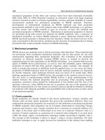
If the vectors A, B, and C coincide with the edges of a parallelepiped as in Figure 2.8.1,
the scalar triple product of A, B, and C is seen to be equal to the volume of the parallel-
epiped. That is, the volume V is:
(2.8.6)
Example 2.8.1: Verification of Interchangeability of Terms of Triple Scalar
Products
Let vectors A, B, and C be expressed in terms of mutually perpendicular unit vectors n
1
,
n
2
, and n
3
as:
(2.8.7)
Verify the equalities of Eq. (2.8.5).
Solution: From Eq. (2.8.2), the vector products A × B and B × C are:
(2.8.8)
(2.8.9)

Then, from Eq. (2.6.22), the triple scalar products A × B · C and B × C · A are:
(2.8.10)
and
(2.8.11)
The other equalities are verified similarly (see Problem P2.8.1).
Next, the vector triple product has one of the two forms: A × (B × C) or (A × B) × C.
The result is a vector. The position of the parentheses is important, as the two forms
generally produce different results.
To explore this, let the vectors A, B, and C be expressed in terms of mutually perpen-
dicular unit vectors n
i
with scalar components A
i
, B
i
, and C
i
(i = 1, 2, 3). Then, by using
FIGURE 2.8.1
A parallelepiped with vectors A, B,
and C along the edges.
B
A
C
V =×⋅ABC
AnnnBnnnCnnn=− − + = + − =− + −324735
123 1 2 3 1 2 3
, ,
AB
nnn

nnn×= −
−
=+ +
123
123
311
24 7
32314
BC
nnn
nnn×= −
−−
=+ +
123
123
24 7
13 5
17 10
ABC×⋅=
()
−
()
+
()()
+
()
−
()
=−3 1 23 3 14 5 4
BCA×⋅=

()()
+
()
−
()
+
()()
=−1 3 17 1 10 1 4
0593_C02_fm Page 35 Monday, May 6, 2002 1:46 PM
36 Dynamics of Mechanical Systems
the algorithms of Eqs. (2.8.1) and (2.8.2), we see that the vector triple products may be
expressed as:
(2.8.12)
and
(2.8.13)
Observe that the last terms in these expressions are different.
Example 2.8.2: Validity of Eqs. (2.8.6) and (2.8.7) and the Necessity of
Parentheses
Verify Eqs. (2.8.6) and (2.8.7) using the vectors of Eq. (2.8.7).
Solution: From Eqs. (2.8.2) and (2.8.9), A × (B × C) is:
(2.8.14)
From Eq. (2.6.22), (A · C)B – (A · B)C is:
(2.8.15)
Similarly, (A × B) × C and (A · C)B – (B · C)A are:
(2.8.16)
and
(2.8.17)
ABC ACBABC×⋅
()
=⋅

()
−⋅
()
AB C ACB BCA×
()
×= ⋅
()
−⋅
()
ABC
nnn
nnn××
()
=− =−−+
123
123
311
11710
27 29 52
ACB ACC n n n
nnn
nnn
n
⋅
()
−⋅
()
=
()
−

()
+−
()()
+
()
−
()
[]
+−
()
−
()()
+−
()()
+
()
−
()
[]
−+ −
()
=−
()
+−
()
−−
()
−+
31 13 152 4 7
32 14 1 7 3 5

11 2 4 7
5
123
123
123
1
335
27 29 52
23
123
nn
nnn
−
()
=− − +
AB C
nnn
nn n×
()
×=
−−
=− + +
123
12 3
32314
13 5
157 32
ACB BCA n n n
nnn
nnn

n
⋅
()
−⋅
()
=
()
−
()
+−
()()
+
()
−
()
[]
+−
()
−
()
−
()
+
()()
+−
()
−
()
[]
−+

()
=−
()
+−
()
−
()
−
31 13 152 4 7
21 43 753
11 2 4 7
45 3
123
123
123
1

nnn
nn n
23
12 3
157 32
+
()
=− + +
0593_C02_fm Page 36 Monday, May 6, 2002 1:46 PM
Review of Vector Algebra 37
Observe that the results in Eqs. (2.8.14) and (2.8.15) are identical and thus consistent
with Eq. (2.8.12). Similarly, the results of Eqs. (2.8.16) and (2.8.17) are the same, thus
verifying Eq. (2.8.13). Finally, observe that the results of Eqs. (2.8.14) and (2.8.16) are

different, thus demonstrating the necessity for parentheses on the left sides of Eqs. (2.8.12)
and (2.8.13).
Recall from Eq. (2.6.10) that the projection A

of a vector A along a line L is:
(2.8.18)
where n is a unit vector parallel to L, as in Figure 2.8.2. The vector triple product may be
used to obtain A
⊥
, the component of perpendicular to L. That is,
(2.8.19)
To see this, use Eqs. (2.8.6) and (2.8.8) to expand the product. That is,
(2.8.20)
2.9 Use of the Index Summation Convention
Observe in the previous sections that expressing a vector in terms of mutually perpendic-
ular unit vectors results in a sum of products of the scalar components and the unit vectors.
Specifically, if v is any vector and if n
1
, n
2
, and n
3
are mutually perpendicular unit vectors,
we can express v in the form:
(2.9.1)
Because these sums occur so frequently, and because the pattern of the indices is similar
for sums of products, it is convenient to introduce the “summation convention”: if an
index is repeated, there is a sum over the range of the index (usually 1 to 3). This means,
for example, in Eq. (2.9.1), that the summation sign may be deleted. That is, v may be
expressed as:

(2.9.2)
FIGURE 2.8.2
Projection of a vector A parallel and
perpendicular to a line.
L
n
A
A
A
⊥
࿣
AAnn
||
=⋅
()
AnAn
⊥
=× ×
()
nAn An nAA A××
()
=−⋅
()
=− =
⊥
A
||
v nnn n=− + + =
=
∑

vvv v
ii
i
11 21 33
1
3
Vn= v
ii
0593_C02_fm Page 37 Monday, May 6, 2002 1:46 PM
38 Dynamics of Mechanical Systems
In using this convention, several rules are useful. First, in an equation or expression, a
repeated index may not be repeated more than one time. Second, any letter may be used
for a repeated index. For example, in Eq. (2.9.2) we may write:
(2.9.3)
Finally, if an index is not repeated it is a “free” index. In an equation, there must be a
correspondence of free indices on both sides of the equation and in each term of the
equation.
In using the summation convention, we can express the scalar and vector products as
follows: If n
1
, n
2
, and n
3
are mutually perpendicular unit vectors and if vectors a and b
are expressed as:
(2.9.4)
then the products a · b and a × b are:
(2.9.5)
where, as before, e

ijk
is the permutation symbol (see Eq. (2.7.7)).
With a little practice, the summation convention becomes natural in analysis procedures.
We will employ it when it is convenient.
Example 2.9.1: Kronecker Delta Function Interpreted
as a Substitution Symbol
Consider the expression δ
ij
V
j
where the δ
ij
(i, j = 1, 2, 3) are components of the Kronecker
delta function defined by Eq. (2.6.7) and where V
j
are the components of a vector V relative
to a mutually perpendicular unit vector set n
i
(i = 1, 2, 3). From the summation convention,
we have:
(2.9.6)
In this equation, i has one of the values 1, 2, or 3. If i is 1, the right side of the equation
reduces to V
1
; if i is 2, the right side becomes V
2
; and, if i is 3, the right side is V
3
. Therefore,
the right side is simply V

i
. That is,
(2.9.7)
The Kronecker delta function may then be interpreted as an index operator, substituting
an i for the j, thus the name substitution symbol.
2.10 Review of Matrix Procedures
In continuing our review of vector algebra, it is helpful to recall the elementary procedures
in matrix algebra. For illustration purposes, we will focus our attention primarily on square
vn n n===vvv
ii jj
kk
an bn==ab
ii ii
and
ab a b n⋅= ×=a b and e a b
ii
ijk
ij
k

δδδ δ
ij j i i i
VVVVi=++ =
()
11 22 33
123 , ,
δ
ij j i
VV=
0593_C02_fm Page 38 Monday, May 6, 2002 1:46 PM

Review of Vector Algebra 39
matrices and on row and column arrays. Recall that a matrix A is simply an array of
numbers a
ij
(i = 1,…, m
i
; j = 1,…, n) arranged in m rows and n columns as:
(2.10.1)
The entries a
ij
are usually called the elements of the matrix. The first subscript indicates
the row position, and the second subscript designates the column position.
Two matrices A and B are said to be equal if they have equal elements. That is,
(2.10.2)
If all the elements of matrix are zero, it is called a zero matrix. If a matrix has only one
row, it is called a row matrix or row array. If a matrix has only one column, it is called a
column matrix or column array. A matrix with an equal number of rows and columns is a
square matrix. If all the elements of a square matrix are zero except for the diagonal
elements, the matrix is called a diagonal matrix. If all the diagonal elements of a diagonal
matrix have the value 1, the matrix is called an identity matrix. If a square matrix has a
zero determinant, it is said to be a singular matrix. The transpose of a matrix A (written A
T
)
is the matrix obtained by interchanging the rows and columns of A. If a matrix and its
transpose are equal, the matrix is said to be symmetric. If a matrix is equal to the negative
of its transpose, it is said to be antisymmetric.
Recall that the algebra of matrices is based upon a few simple rules: First, the multipli-
cation of a matrix A by a scalar s produces a matrix B whose elements are equal to the
elements of A multiplied by s. That is,
(2.10.3)

Next, the sum of two matrices A and B is a matrix C whose elements are equal to the
sum of the respective elements of A and B. That is,
(2.10.4)
Matrix subtraction is defined similarly.
The product of matrices is defined through the “row–column” product algorithm. The
product of two matrices A and B (written AB) is possible only if the number of columns
in the first matrix A is equal to the number of rows of the second matrix B. When this
occurs, the matrices are said to be conformable. If C is the product AB, then the element c
ij
is the sum of products of the elements of the ith row of A with the corresponding elements
of the jth column of B. Specifically,
(2.10.5)
where n is the number of columns of A and the number of rows of B.
A
aa an
aa an
aa a
mn mn
=













11 12 1
21 22 2
12




AB a b i nj m
ij ij
==== , , ; , , if and only if 1 1
BsA b sa
ij ij
== if and only if
CAB c a b
ij ij ij
=+ =+ if andonlyif
cab
ij
ik kj
k
n
=
=
∑
1
0593_C02_fm Page 39 Monday, May 6, 2002 1:46 PM
40 Dynamics of Mechanical Systems
Matrix products are distributive over addition and subtraction. That is,
(2.10.6)

and
(2.10.7)
Matrix products are also associative. That is, for conformable matrices A, B, and C, we
have:
(2.10.8)
Hence, the parentheses are unnecessary.
Next, it is readily seen that the transpose of a product is the product of the transposes
in reverse order. That is:
(2.10.9)
Finally, if A is a nonsingular square matrix, the inverse of A, written as A
–1
, is the matrix
such that:
(2.10.10)
where I is the identity matrix. A
–1
may be determined as follows: Let M
ij
be the minor of
the element a
ij
defined as the determinant of the matrix occurring when the ith row of A
and the jth column of a are deleted. Let Â
ij
be the adjoint of a
ij
defined as:
(2.10.11)
Then A
–1

is the matrix with elements:
(2.10.12)
where detA designates the determinant of A and [Â
ij
]
T
is the transpose of the matrix of
adjoints.
If it happens that:
(2.10.13)
then A is said to be orthogonal. In this case, the rows and columns of A may be considered
as components of mutually perpendicular unit vectors.
AB C AB AC+
()
=+
BCA BACA+
()
=+
AB C A BC ABC
()
=
()
=
AB B A
T
TT
()
=
AA A A I
−−

==
11
ˆ
AM
ij
ij
ij
=−
()
+
1
AA A
ij
T
−
=
[]
1
ˆ
det
AA
T−
=
1
0593_C02_fm Page 40 Monday, May 6, 2002 1:46 PM
Review of Vector Algebra 41
2.11 Reference Frames and Unit Vector Sets
In the analysis of dynamical systems, it is frequently useful to express kinematical and
dynamical quantities in several different reference frames. Orthogonal transformation
matrices (as discussed in this section) are useful in obtaining relationships between the

representations of the quantities in the different reference frames.
To explore these ideas consider two unit vector sets n
i
and
i
and an arbitrary V as in
Figure 2.11.1. Let the sets be inclined relative to each other as shown. Recall from
Eq. (2.6.19) that V may be expressed in terms of the n
i
as:
(2.11.1)
where the V
i
are the scalar components of V. Similarly, V may be expressed in terms of
the
i
as:
(2.11.2)
Given the relative inclination of the unit vector sets, our objective is to obtain relations
between the V
i
and the
i
. To that end, let S be a matrix with elements S
ij
defined as:
(2.11.3)
Consider the n
i
: from Eq. (2.11.2), we can express n

i
as:
(2.11.4)
Similarly, n
2
and n
3
may be expressed as:
(2.11.5)
Thus, in general, we have:
(2.11.6)
FIGURE 2.11.1
Two unit vector sets.
ˆ
n
V Vn n Vn n Vn n Vn n Vn=⋅
()
+⋅
()
+⋅
()
=⋅
()
=
11 22 33 ii ii
ˆ
n
VVnnVn=⋅
()
=

ˆˆ
ˆ
ˆ
ii ii
ˆ
V
S
ij i j
=⋅nn
ˆ
nnnn n
11 1
=⋅
()
=
ˆˆ ˆ
ii ii
S
nn nn
22 33
==SS
ii ii
ˆˆ
and
nn
iijj
S=
ˆ
V
n

n
n
n
n
n
3
1
2
3
2
1
ˆ
ˆ
ˆ
0593_C02_fm Page 41 Monday, May 6, 2002 1:46 PM
42 Dynamics of Mechanical Systems
Similarly, if we express
1
,
2
, and
3
in terms of the
i
, we have:
(2.11.7)
Observe the difference between Eqs. (2.11.6) and (2.11.7): in Eq. (2.11.6), the sum is taken
over the second index of S
ij
, whereas in Eq. (2.11.7) it is taken over the first index. This is

consistent with Eq. (2.11.3), where we see that the first index is associated with the n
i
and
the second with the
i
. Observe the same pattern in Eqs. (2.11.6) and (2.11.7).
By substituting from Eqs. (2.11.6) and (2.11.7) into Eqs. (2.11.1) and (2.11.2), we obtain:
(2.11.8)
and
(2.11.9)
Hence, we have:
(2.11.10)
Observe that Eq. (2.11.10) has the same form as Eqs. (2.11.6) and (2.11.7).
By substituting from Eqs. (2.11.6) and (2.11.7), we obtain the expression:
(2.11.11)
where, as in Eq. (2.6.7), δ
ik
is Kronecker’s delta function. In matrix form, this may be
written as:
(2.11.12)
where, as before, I is the identity matrix. Hence, S is an orthogonal transformation matrix
(see Eq. (2.10.12)).
To illustrate these ideas, imagine the unit vector sets n
i
and
i
to be aligned with each
other such that n
i
and

i
are parallel (i = 1, 2, 3). Next, let the
i
be rotated relative to the
n
i
and
i
so that the angle between
2
and n
2
(and also between
3
and n
3
) is α, as shown
in Figure 2.11.2. Then, by inspection of the figure, n
i
and
i
are related by the expressions:
(2.11.13)
ˆ
n
ˆ
n
ˆ
n
ˆ

n
ˆ
nn
iijj
S=
ˆ
n
Vn n n== =VV V
ii iijj jj
S
ˆˆ
ˆ
ˆ
Vn n n== =
ˆ
ˆ
ˆ
VV V
ii iijj jj
S
V V and V
iijj ijij
SSV==
ˆˆ
SS SS
ij
kj ik
ji
jk ik
==δδ and

SS S S I S S
TT T
== =
−
or
1
ˆ
n
ˆ
n
ˆ
n
ˆ
n
ˆ
n
ˆ
n
ˆ
n
nn
nnn
nnn
nn
nnn
nnn
11
23
323
11

23
323
=
=+
=+
=
=+
=− +
ˆ
ˆ
ˆˆ
ˆ
ˆ
ˆ
22
andcs
sc
cs
sc
αα
αα
αα
αα
0593_C02_fm Page 42 Monday, May 6, 2002 1:46 PM
Review of Vector Algebra 43
where s
α
and c
α
represent sinα and cosα. Hence, from Eq. (2.11.3), the matrix S has the

elements:
(2.11.14)
Observe that SS
T
and S
T
S are:
(2.11.15)
and
(2.11.16)
Observe in Figure 2.11.2 the rotation of the
i
and
1
through the angle α is a dextral
rotation. Imagine analogous dextral rotations of the
i
about
2
and
3
through the angles
β and γ. Then, it is readily seen that the transformation matrices analogous to S of Eq.
(2.11.14) are:
(2.11.17)
(In this context, the transformation matrix of Eq. (2.11.15) might be called A.)
Finally, let the
i
have a general inclination relative to the n
i

as shown in Figure 2.11.1.
The
i
may be brought into this configuration by initially aligning them with the n
i
and
FIGURE 2.11.2
Unit vector sets n
i
and
ˆ
n
i
.
α
α
n
n
n n
n
n
ˆ
ˆ
ˆ
3
3
2
2
1
1

,
SS c s
sc
ij
=
[]
=−










10 0
0
0
αα
αα
SS c s
sc
cs
sc
T
=−











−










=











10 0
0
0
10 0
0
0
100
010
001
αα
αα
αα
αα
SS c s
sc
cs
sc
T
=
−











−










=










10 0
0
0
10 0
0
0
100
010

001
αα
αα
αα
αα
ˆ
n
ˆ
n
ˆ
n
ˆ
n
ˆ
n
B
cs
sc
C
s
sc=
−











=
−










ββ
ββ
γγ
γγ
0
010
0
0
0
001
and
c
ˆ
n
ˆ
n

0593_C02_fm Page 43 Monday, May 6, 2002 1:46 PM
44 Dynamics of Mechanical Systems
then by performing three successive dextral rotations of the
i
about
1
,
2
, and
3
through
the angles α, β, and γ. The transformation matrix S between the n
i
and the
i
is, then:
(2.11.18)
or,
(2.11.19)
Also, it is readily seen that:
(2.11.20)
and that:
(2.11.21)
2.12 Closure
The foregoing discussion is intended primarily as a review of basic concepts of vector and
matrix algebra. Readers who are either unfamiliar with these concepts or who want to
explore the concepts in greater depth may want to consult a mathematics or vector
mechanics text as provided in the References. We will freely employ these concepts
throughout this text.
References

2.1. Hinchey, F. A., Vectors and Tensors for Engineers and Scientists, Wiley, New York, 1976.
2.2. Hsu, H. P., Vector Analysis, Simon & Schuster Technical Outlines, New York, 1969.
2.3. Haskell, R. E., Introduction to Vectors and Cartesian Tensors, Prentice Hall, Englewood Cliffs, NJ,
1972.
2.4. Shields, P. C., Elementary Linear Algebra, Worth Publishers, New York, 1968.
2.5. Ayers, F., Theory and Problems of Matrices, Schawn Outline Series, McGraw-Hill, New York,
1962.
2.6. Pettofrezzo, A. J., Elements of Linear Algebra, Prentice Hall, Englewood Cliffs, NJ, 1970.
2.7. Usamani, R. A., Applied Linear Algebra, Marcel Dekker, New York, 1987.
2.8. Borisenko, A. I., and Tarapov, I. E., Vector and Tensor Analysis with Applications (translated by
R. A. Silverman), Prentice Hall, Englewood Cliffs, NJ, 1968.
ˆ
n
ˆ
n
ˆ
n
ˆ
n
ˆ
n
S ABC c s
sc
cs
sc
cs
sc== −











−










−










10 0

0
0
0
010
0
0
0
001
αα
αα
ββ
ββ
γγ
γγ
S
cc cs s
cs ssc cc sss sc
ss csc sc css cc
=
−
+
()
−
()
−
−
()
+
()













β
γ
β
γ
β
αγ α
β
γαγα
β
γα
β
αγ α
β
γαγα
β
γα
β
SCBA
TTTT

=
SS S S I
TT
==
0593_C02_fm Page 44 Monday, May 6, 2002 1:46 PM
Review of Vector Algebra 45
Problems
Section 2.3 Vector Addition
P2.3.1: Given the vectors A, B, C, and D as shown in Figure P2.3.1, let the magnitudes of
these vectors be:
A = 8 lb, B = 6 lb, C = 12 lb, D = 5 lb
Find the magnitudes of the following sums:
a. A + B
b. B + A
c. 2A + 2B
d. A – B
e. A + C
f. B + C
g. A + B + C
h. C + D
i. B + D
j. A + B + C + D
k. 3A – 2B + C – 4D
l. D – 4A + B
Section 2.4 Vector Components
P2.4.1: Given the unit vectors i and j and the vectors A and B as shown in Figure P2.4.1,
let the magnitudes of A and B be 10 N and 15 N, respectively. Express A and B in terms
of i and j.
P2.4.2: See Problem P2.4.1. Let C be the resultant (or sum) of A and B.
a. Express C in terms of the unit vectors i and j.

b. Find the magnitude of C.
FIGURE P2.3.1
A set of four vectors.
A
B
C
D
45°
45°
0593_C02_fm Page 45 Monday, May 6, 2002 1:46 PM
46 Dynamics of Mechanical Systems
P2.4.3: Given the unit vectors i and j and the vectors A and B as shown in Figure P2.4.3,
let the magnitudes of A and B be 15 lb and 26 lb, respectively. Express A and B in terms
of i and j.
P2.4.4: See Problem 2.4.3. Let C be the resultant of A and B.
a. Express C in terms of i and j.
b. Find the magnitude of C.
P2.4.5: Given the Cartesian coordinate system as shown in Figure P2.4.5, let A, B, and C
be points in space as shown. Let n
x
, n
y
, and n
z
be unit vectors parallel to X, Y, and Z.
a. Express the position vectors AB, BC, and CA in terms of n
x
, n
y
, and n

z
.
b. Find unit vectors parallel to AB, BC, and CA.
P2.4.6: See Problem P2.4.5. Let R be the resultant of AB, BC, and CA. Express R in terms
of n
x
, n
y
, and n
z
.
FIGURE P2.4.1
Vectors A and B and a unit vector.
FIGURE P2.4.3
Vectors A and B and unit vectors.
FIGURE P2.4.5
A Cartesian coordinate system with points
A, B, and C.
Y
X
j
i
A
B
30°
45°
|A| = 10 N
|B| = 15 N
Y
X

j
i
A
B
3
4
5
12
Z
Y
X
O
A(3,-1,4)
B(1,3,3)
C(4,6,-1)
n
n
n
z
y
x
0593_C02_fm Page 46 Monday, May 6, 2002 1:46 PM
Review of Vector Algebra 47
P2.4.7: See Figure P2.4.7. Forces F
1
,…, F
6
act along the edges and diagonals of a parallel-
epiped (or box) as shown. Let i, j, and k be mutually perpendicular unit vectors parallel
to the edges of the box. Let the box be 12 inches long, 3 inches high, and 4 inches deep.

Let the magnitudes of F
1
,…, F
6
be:
a. Find unit vectors n
1
,…, n
6
parallel to the forces F
1
,…, F
6
. Express these unit vectors
in terms of i, j, and k.
b. Express F
1
,…, F
6
in terms of unit vectors n
1
,…, n
6
.
c. Express F
1
,…, F
6
in terms of i, j, and k.
d. Find the resultant R of F

1
. Express R in terms of i, j, and k.
e. Find the magnitude of R.
P2.4.8: Let forces be given as:
where n
1
, n
2
, and n
3
are mutually perpendicular unit vectors.
a. Find a force F such that the resultant of F and the forces F
1
,…, F
6
is zero. Express
F in terms of n
1
, n
2
, and n
3
.
b. Determine the magnitude of F.
P2.4.9: See Figure P2.4.9. Let P and Q be points of a Cartesian coordinate system with
coordinates as shown. Let n
x
, n
y
, and n

z
be unit vectors parallel to the coordinate axes as
shown.
FIGURE P2.4.7
Forces acting along the edges and diagonals
of a parallelepiped.
FFF
FFF
123
456
15 18 18
20 17 26
===
===
lb lb lb
lb lb lb


O
C
B
A
12 in E
G
H
D
k
4 in
F
F

F
F
F
3 in
1
5
3
4
2
F
6
i
j
Fnnn
Fnnn
Fnnn
Fnnn
Fnnn
1123
2123
3123
4123
5123
32
462
34
783
549
=−+
=+−

=− + +
=−+
=− + −
N
N
N
N
N
0593_C02_fm Page 47 Monday, May 6, 2002 1:46 PM
48 Dynamics of Mechanical Systems
a. Construct the position vectors OP, OQ, and PQ and express the results in terms
of n
x
, n
y
, and n
z
.
b. Determine the distance between P and Q if the coordinates are expressed in
meters.
c. Find the angles between OP and the X-, Y-, and Z-axes.
d. Find the angles between OQ and the X-, Y-, and Z-axes.
e. Find the angles between PQ and the X-, Y-, and Z-axes.
Section 2.5 Angle Between Two Vectors
P2.5.1: From the definition in Section 2.5, what is the angle between two parallel vectors
with the same sense? What is the angle if the vectors have opposite sense? What is the
angle between a vector and itself?
Section 2.6 Vector Multiplication: Scalar Product
P.2.6.1: Consider the vectors A and B shown in Figure P2.6.1. Let the magnitudes of A
and B be 8 and 5, respectively. Evaluate the scalar product A · B.

P2.6.2: See Problem P2.6.1 and Figure P2.6.1. Express A and B in terms of the unit vectors
n
1
and n
2
as shown in the figure. Use Eq. (2.6.2) to evaluate A · B.
P2.6.3: See Problems P2.6.1 and P2.6.2. Let C be the resultant of A and B. Find the
magnitude of C.
P2.6.4: Let n
1
, n
2
, and n
3
be mutually perpendicular unit vectors. Let vectors A and B be
expressed in terms of n
1
, n
2
, and n
3
as:
FIGURE P2.4.9
A Cartesian coordinate system with
points P and Q.
FIGURE P2.6.1
Vectors A and B.
P(0.5,1,3)
Q(2,5,2)
O

Z
Y
X
n
n
n
z
y
x
120°
B
A
n
n
|A| = 8
|B| = 5
2
1
Annn Bnnn=−++ =−+356 427
123 123
and
0593_C02_fm Page 48 Monday, May 6, 2002 1:46 PM
Review of Vector Algebra 49
a. Determine the magnitudes of A and B.
b. Find the angle between A and B.
P2.6.5: Let vectors A and B be expressed in terms of mutually perpendicular unit vectors as:
Find B
y
so that the angle between A and B is 90˚.
P2.6.6: See Figure P2.6.6. Let the vector V be expressed in terms of mutually perpendicular

unit vectors n
x
, n
y
, and n
z
, as:
Let the line L pass through points A and B where the coordinates of A and B are as shown.
Find the projection of V along L.
P2.6.7: A force F is expressed in terms of mutually perpendicular unit vectors n
x
, n
y
, and
n
z
as:
If F moves a particle P from point A (1, –2, 4) to point B (–3, 4, –5), find the projection of
F along the line AB, where the coordinates (in feet) of A and B are referred to an X, Y, Z
Cartesian system and where n
x
, n
y
, and n
z
are parallel to X, Y, and Z.
P2.6.8: See Problem P2.6.7. Let the work W done by F be defined as the product of the
projection of F along AB and distance between A and B. Find W.
Section 2.7 Vector Multiplication: Vector Product
P2.7.1: Consider the vectors A and B shown in Figure P2.7.1. Using Eq. (2.7.1), determine

the magnitude of the vector product A × B.
a. If A and B are in the X–Y plane, what is the direction of A × B?
b. What is the direction of B × A?
FIGURE P2.6.6
A vector V and a line L.
Ann n BnBnn=+− =+ +45 2
12 3 1 23
and
y
Vn n n=+−342
xyz
O
Z
Y
X
n
n
n
z
y
x
V
B(1,7,3)
L
A(2,1,2)
Fnnn=− + −427
xyz
lb
0593_C02_fm Page 49 Monday, May 6, 2002 1:46 PM
50 Dynamics of Mechanical Systems

P2.7.2: See Problem P2.7.1. What is the magnitude of 6A × 2B?
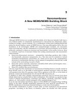
P2.7.3: Consider the vectors A, B, and C shown in Figure P2.7.3. Let i, j, and k be mutually
perpendicular unit vectors as shown, with k being along the Z-axis.
a. Evaluate the sum B + C.
b. Determine the vector products A × B and A × C.
c. Use the results of (b) to determine the sum of A × B and A × C.
d. Use the results of (a) to determine the product A × (B + C). Compare the result
with that of (c).
P.2.7.4: Let n
1
, n
2
, and n
3
be mutually perpendicular (dextral) unit vectors, and let vectors
A, B, and C be expressed in terms of n
1
, n
2
, and n
3
as:
a. Evaluate the sum B + C.
b. Use Eq. (2.7.24) to determine the vector products A × B and A × C.
c. Use the results of (b) to determine the sum of A × B and A × C.
d. Use the results of (a) to determine the product A × (B + C). Compare the result
with that of (c).
FIGURE P2.7.1
Vectors A and B in the X–Y plane.
FIGURE P2.7.3

Vectors A, B, and C in the X–Y plane.
Y
X
A
B
30°
|A| = 45
|B| = 30
Y
X
A
B
30°
|A| = 45
|B| = 30
30°
C
O
k
j
i
|C| = 35
Annn
Bnnn
Cn n n
=−+
=− + −
=+−
6
542

357
123
122
123
0593_C02_fm Page 50 Monday, May 6, 2002 1:46 PM
Review of Vector Algebra 51
P2.7.5: Let A and B be expressed in terms of mutually perpendicular unit vectors n
1
, n
2
,
and n
3
as:
Find a unit vector perpendicular to A and B.
P2.7.6: See Figure P2.7.6. Let X, Y, and Z be mutually perpendicular coordinate axes, and
let A, B, and C be points with coordinates relative to X, Y, and Z as shown.
a. Form the position vectors AB, BC, and CA, and express the results in terms of
the unit vectors n
x
, n
y
, and n
z
.
b. Evaluate the vector products AB × BC, BC × CA, and CA × AB.
c. Find a unit vector n perpendicular to the triangle ABC.
P2.7.7: See Figure P2.7.7. Let LP and LQ be lines passing through points P
1
, P

2
and Q
1
, Q
2
as shown. Let the coordinates of P
1
, P
2
, Q
1
, and Q
2
relative to the X, Y, Z system be as
shown. Find a unit vector n perpendicular to LP and LQ, and express the results in terms
of the unit vectors n
x
, n
y
, and n
z
shown in Figure P2.7.7.
P2.7.8: See Figure P2.7.8. Let points P and Q have the coordinates (in feet) as shown. Let
L be a line passing through P and Q, and let F be a force acting along L. Let the magnitude
of F be 7 lb.
FIGURE P2.7.6
A triangle ABC in an X, Y, Z reference
frame.
FIGURE P2.7.7
Lines LP and LQ in an X, Y, Z reference

frame.
An n n
Bnn n
=−+
=−−
368
45
123
12 3
O
Z
Y
X
A(1,1,4)
B(3,7,5)
C(2,5,1)
n
n
n
z
x
y
Z
Q (-1,-2,7)
n
P (3,-1,3)
X
n
n
Y

L
L
P (0,6,4)
Q (4,5,2)
1
2
1
2
z
x
y
P
Q
0593_C02_fm Page 51 Monday, May 6, 2002 1:46 PM
52 Dynamics of Mechanical Systems
a. Find a unit vector n parallel to L, in the direction of P to Q. Express the results
in terms of the unit vectors n
x
, n
y
, and n
z
shown in Figure P2.7.7.
b. Express F in terms of n
x
, n
y
, and n
z
.

c. Form the vectors OP and OQ, calculate OP × F and OQ × F, and express the
results in terms of n
x
, n
y
, and n
z
. Compare the results.
P2.7.9: Let e
ijk
and δ
jk
be the permutation symbol and the Kronecker delta symbol as in
Eqs. (2.7.7) and (2.6.7). Evaluate the sums:
Section 2.8 Vector Multiplication: Triple Products
P2.8.1: See Example 2.8.1. Verify the remaining equalities of Eq. (2.8.5) for the vectors A,
B, and C of Eq. (2.8.7).
P2.8.2: Use Eq. (2.8.6) to find the volume of the parallelepiped shown in Figure P2.8.2,
where the coordinates are measured in meters.
P2.8.3: The triple scalar product is useful in determining the distance d between two non-
parallel, non-intersecting lines. Specifically, d is the projection of a vector P
1
P
2
, which
connects any point P
1
on one of the lines with any point P
2
on the other line, onto the

common perpendicular between the lines. Thus, if n is a unit vector parallel to the common
perpendicular, d is given by:
FIGURE P2.7.8
Coordinate system X, Y, Z with points P
and Q, line L, and force F.
FIGURE P2.8.2
Parallelepiped.
Z
n
X
n
n
Y
z
x
y
O
F
L
Q (2,4,1)
P (1,-1,3)
F = 7 lb
ei
ijk jk
kj
δ ,,=
==
∑∑
123
1

3
1
3
Z
Y
X
O
k
i
j
A(6,0,0)
C(1,1,5)
B(2,8,0)
d =⋅PP n
12
0593_C02_fm Page 52 Monday, May 6, 2002 1:46 PM
Review of Vector Algebra 53
Using these concepts, find the distance d between the lines L
1
and L
2
shown in Figure
P2.8.3, where the coordinates are expressed in feet. (Observe that n may be obtained from
the vector product (P
1
Q
1
× P
2
Q

2
)/P
1
Q
1
× P
2
Q
2
.)
P2.8.4: The triple vector product is useful in determining second-moment vectors. Let P
be a particle with mass m located at a point P with coordinates (x, y, z) relative to a Cartesian
coordinate frame X, Y, Z, as in Figure P2.8.4. (If a particle is small, it may be identified by
a point.) Let position vector p locate P relative to the origin O. Let n
a
be an arbitrarily
directed unit vector and let n
x
, n
y
, and n
z
be unit vectors parallel to axes X, Y, and Z as
shown. The second moment vector I
a
of P for O for the direction n
a
is then defined as:
a. Show that in this expression the parentheses are unnecessary; that is, unlike the
general triple vector products in Eqs. (2.8.12) and (2.8.13), we have here:

b. Observing that p may be expressed as:
find I
x
, I
y
, and I
z
, the second moment vectors for the directions n
x
, n
y
, and n
z
.
FIGURE P2.8.3
Distance d between non-parallel,
non-intersecting lines.
FIGURE P2.8.4
A particle P in a Cartesian reference frame.
d
n
Q (0,6,3)
Q (1,5,0)
P (2,-2,4)
P (6,-1,4)
O
X
n
n
n

Y
z
x
y
1
1
2
2
Z
Ipnp
aa
m=××
()
n
O
X
n
n
n
Y
z
x
y
Z
P(x,y,z)
p
a
mmn
aa
pnp p p××

()
=×
()
×
pn n n=++xyz
xyz
0593_C02_fm Page 53 Monday, May 6, 2002 1:46 PM
54 Dynamics of Mechanical Systems
c. Let unit vector n
a
be expressed in terms of n
x
, n
y
, and n
z
as:
show that I
a
may then be expressed as:
Section 2.9 Use of the Index Summation Convention
P2.9.1: Evaluate and/or expand the following terms:
a. δ
kk
b. e
ijk
δ
jk
c. a
ij

b
jk
Section 2.10 Review of Matrix Procedures
P2.10.1: Given the matrices A, B, and C:
a. Compute the products AB and BC.
b. Compute the products (AB)C and A(BC) and compare the results (see Eq.
(2.8.10)).
c. Find B
T
, A
T
, and the product B
T
A
T
.
d. Find (AB)
T
and compare with B
T
A
T
(see Eq. (2.10.9)).
e. Find , the matrix of adjoints for A (see Eq. (2.10.11)).
f. Compute A
–1
.
g. Compute the products A
–1
A and AA

–1
.
P2.10.2: Given the matrix S (an orthogonal matrix):
a. Find detS.
b. Find S
–1
.
c. Find S
T
.
d. Compare S
–1
and S
T
.
nnnn
axxyyzz
aaa=++
IIII
axxyyzz
aaa=++
AB C=
−
−











=
−
−










=
−−
−











124
583
769
48 3
569
05 2
717
36 8
429

ˆ
A
S =−
−










12 6 4 6 4
32 24 24
02222
0593_C02_fm Page 54 Monday, May 6, 2002 1:46 PM
Review of Vector Algebra 55
Section 2.11 Reference Frames and Unit Vector Sets

P2.11.1: Determine the numerical values of the transformation matrix elements of
Eq. (2.11.19) if α, β, and γ have the values:
P2.11.2: See Problem P2.11.1. Show that S
T
= S
–1
and that detS = 1.
αβγ=° =° =°30 45 60, ,
0593_C02_fm Page 55 Monday, May 6, 2002 1:46 PM
0593_C02_fm Page 56 Monday, May 6, 2002 1:46 PM