Adaptive Control System Part 3 ppsx
Bạn đang xem bản rút gọn của tài liệu. Xem và tải ngay bản đầy đủ của tài liệu tại đây (240.5 KB, 25 trang )
at
1 t À d
T
Pt À 1t À d
Â
1
1 À
t
2
À et
2
1
1 À
tÀtQt
!
at
1 t À d
T
Pt À 1t À d
À et
2
1
1 À
tQt
!
at
1 t À d
T
Pt À 1t À d
À et
2
1
1 À
1
et
2
!
at
1 t À d
T
Pt À 1t À d
À et
2
1
0
et
2
!
À
0
À 1
0
at
1 t À d
T
Pt À 1t À d
et
2
À
0
À 1
0
f t
2
1 t À d
T
Pt À 1t À d
2:18
where the fact that atet
2
f tet!f t
2
has been used. Therefore,
following the same arguments in [20], [21], [23], the results in Lemma 4.1 are
thus proved.
If using the same adaptive control law as in equation (2.11), then with the
parameter estimation properties (i)±(v) in Lemma 4.1, the global stability and
convergence results of the new adaptive control system can be established as in
[26], [11] as long as the estimated
"
"
1
is small enough, which are summarized in
the following theorem.
Theorem 4.1 The direct adaptive control system satisfying assumptions (A1)±
(A4) with the adaptive controller described in equations (2.7), (2.9), (2.13)±
(2.16) and (2.11) is globally stable in the sense that all the signals in the loop
remain bounded.
In this approach, we have eliminated the requirement for the knowledge of
the parameters of the upper bounding function on the modelling uncertainties.
But the requirement for the knowledge of the lower bound on the leading
coecient of the parameter vector, i.e. assumption (A4) is still there. In the
next section, the technique of the parameter correction procedure will be
combined with the algorithm developed in this section to ensure the least prior
knowledge on the plant. That is, only assumptions (A1)±(A3) are needed.
Adaptive Control Systems 31
2.5 Robust adaptive control with least prior knowledge
The following modi®ed least squares algorithm will be used for robust
parameter estimation:
t
t À 1at
Pt À 1t À d
1 t À d
T
Pt À 1t À d
"
et
PtPt À 1Àat
Pt À 1t À dt À d
T
Pt À 1
1 t À d
T
Pt À 1t À d
2:19
PÀ1k
0
I; k
0
> 0
and the parameter estimate is then corrected [24] as
"
t
tPtt2:20
where
"
et
"
ytÀ
"
t À 1
T
t À d2:21
the vector t is described in Figure 2.1
where pt is the ®rst column of the covariance matrix Pt, and the term at is
now de®ned as follows:
at
0if
"
etj
2
tQt
f
1=2
tQt
1=2
;
"
et=
"
et otherwise
@
:
with 0 <<1,
2
0
1 À
;
0
> 1, and
Qtt À 1
T
Pt À 1t À d
2
21À1 t À d
T
Pt À1t Àd
sup
0 t
jjxjj
2
1
45
T
sup
0 t
jjxjj
2
1
45
32 An algorithm for robust adaptive control with less prior knowledge
t
t
pt
kptk
"j
1
tj kptk À2j
1
tj
À"kptk
t0
Figure 2.1 Parameter correction vector
And
tis calculated by
t
Ct
T
sup
0 t
jjxjj
2
1
P
R
Q
S
2:22
Ct
Ct À 1
at
1 À 1 t À d
T
Pt À 1t À d
sup
0 t
jjxjj
2
1
P
R
Q
S
;
>0 2:23
where
Ct
T
"
1
"
2
with zero initial condition. It should be noted that
"
1
and
"
2
will be always
positive and non-decreasing.
Remark 5.1 The prediction error
"
et is used in the modi®ed least squares
algorithm to ensure that the estimator property (iii) in the following lemma can
be established.
The properties of the above modi®ed least squares parameter estimator are
summarized in the following lemma.
Lemma 5.1 If the plant satis®es the assumptions (A1)±(A3), the least squares
algorithm (2.19)±(2.23) has the following properties:
(i)
t is bounded, and jj
tÀ
t À 1jj P l
2
.
(ii)
Ct is bounded and non-decreasing, thus converges
(iii)
f
1=2
tQt
1=2
;
"
et
2
1 t À d
T
Pt À 1t À d
P l
2
(iv) jjptjj j
1
tj > b
min
where
b
min
j
1
j
mx1; jj
Ã
jj
with
Ã
de®ned such that
Ã
tPt
Ã
(v) j
"
1
tj >
1 À "
3 "
b
min
(vi)
"
t is bounded, and jj
"
tÀ
"
t À 1jj P l
2
Proof De®ne a Lyapunov function candidate
Vt 1
1
2
~
t
T
Pt
À1
~
t
~
Ct 1
T
À1
~
Ct 1 2:24
Adaptive Control Systems 33
where
~
t
tÀ
Ã
,
~
Ct 1
Ct 1À"
1
"
2
T
. Noting that
"
et
"
ytÀ
"
t À 1
T
t À d
"
ytÀ
t À 1t À dÀt À 1
T
Pt À 1t À d
etÀt À 1
T
Pt À 1t À d2:25
Then, the dierence of the Lyapunov function candidate becomes
Vt 1ÀVt
at
1 t À d
T
Pt À 1t À d
Â
1 t À d
T
Pt À 1t À d
1 1 Àatt À d
T
Pt À 1t À d
ÂtÀt À1
T
Pt À 1t À d
2
À
"
et
2
!
at
~
Ct
T
1 À 1 t À d
T
Pt À 1t À d
sup
0 t
jjxjj
2
1
P
R
Q
S
at
2
1 À
2
1 t À d
T
Pt À 1t À d
2
Â
sup
0 t
jjxjj
2
1
P
R
Q
S
T
sup
0 t
jjxjj
2
1
P
R
Q
S
at
1 t À d
T
Pt À 1t À d
Â
1
1 À
tÀt À 1
T
Pt À 1t À d
2
À
"
et
2
!
2at
tÀt
1 À 1 t À d
T
Pt À 1t À d
at
2
1 À
2
1 t À d
T
Pt À 1t À d
2
Â
sup
0 t
jjxjj
2
1
P
R
Q
S
T
sup
0 t
jjxjj
2
1
P
R
Q
S
34 An algorithm for robust adaptive control with less prior knowledge
at
1 t À d
T
Pt À 1t À d
Â
2
1 À
t
2
À
2
1 À
t À 1
T
Pt À 1t À d
2
À
"
et
2
!
2at
tÀt
1 À 1 t À d
T
Pt À 1t À d
at
2
1À
2
1t À d
T
Pt À1t Àd
2
sup
0 t
jjxjj
2
1
P
R
Q
S
T
sup
0 t
jjxjj
2
1
P
R
Q
S
at
1 t À d
T
Pt À 1t À d
Â
2
1 À
t
2
À
"
et
2
2
1 À
tÀtQt
!
at
1 t À d
T
Pt À 1t À d
À
"
et
2
2
1 À
tQt
!
at
1 t À d
T
Pt À 1t À d
À
"
et
2
2
1 À
1
"
et
2
!
at
1 t À d
T
Pt À 1t À d
À
"
et
2
1
0
"
et
2
!
À
0
À 1
0
at
"
et
2
1 t À d
T
Pt À 1t À d
À
0
À 1
0
f
1=2
tQt
1=2
;
"
et
2
1 t À d
T
Pt À 1t À d
2:26
where the fact that atet
2
f tet!f t
2
has been used. Therefore,
following the same arguments in [26], [11], [21], the results (i)±(iii) in Lemma
5.1 are thus proved. The properties (iv)±(vi) in the lemma can also be obtained
directly from the results in [23].
If using the same adaptive control law as in equation (2.11), then with the
parameter estimation properties (i)±(vi), the global stability and convergence
results of the new adaptive control system can be established as in [26], [11] as
long as the estimated
"
"
1
is small enough, which are summarized in the
following theorem.
Adaptive Control Systems 35
Theorem 5.1 The direct adaptive control system satisfying assumptions (A1)±
(A3) with the adaptive controller described in equations (2.19)±(2.23) and
(2.11) is globally stable in the sense that all the signals in the loop remain
bounded.
2.6 Simulation example
In this section, one numerical example is presented to demonstrate the
performance of the proposed algorithm. A fourth order plant is given by the
transfer function as
GsG
n
sG
u
s
with
G
n
s
5s 2
ss 1
as a nominal part, and
G
u
s
229
s
2
30s 229
as the unmodelled dynamics.
With the sampling period T 0:1 second, we have the following corre-
sponding discrete-time model
Gq
À1
0:09784q
À1
0:1206q
À2
À 0:1414q
À3
À 0:01878q
À4
1 À 2:3422q
À1
1:0788q
À2
À 0:4906q
À3
0:04505q
À4
The reference model is chosen as
G
m
s
1
0:2s 1
whose corresponding discrete-time model is
G
m
q
À1
0:3935q
À1
1 À 0:6065q
À1
We have chosen k
0
1, and
00:6000
T
. If no dead zone is used,
the simulation results are divergent. If using the algorithm developed in this
chapter with 10
À5
, the simulation results are shown as in Figure 2.2, where
(a) represents the system output yt and reference model output y
Ã
t, (b) is
the control signal ut, (c) is the estimated parameter
1
, and (d) denotes the
estimated bounding parameters
"
1
and
"
2
.
In order to demonstrate the eect of the update rate parameter , the
following simulation with 1:4 Â 10
À5
was also conducted. The result is
shown in Figure 2.3.
The steady state values of the several important parameters and the tracking
error in both cases are summarized in Table 2.1.
36 An algorithm for robust adaptive control with less prior knowledge
Adaptive Control Systems 37
Output
and
refe
rence
E
stimate
d
the
ta1
Time in seconds
Time in seconds Time in seconds
Time in seconds
Contr
ol
Est.
b
ound
ing
param
eters
Figure 2.2 Robust adaptive control with 10
À
5
Output
and
re
ferenc
e
Estimated
the
ta1
Contro
l
Est.
bo
unding
p
aramet
ers
Time in secondsTime in seconds
Time in seconds Time in seconds
Figure 2.3 Robust adaptive control with 1:4 Â 10
À5
It can be observed from the above simulation results that the algorithm
developed in this chapter can guarantee the stability of the adaptive system in
the presence of the modelling uncertainties, and the smaller tracking error
could be achieved with smaller update rate parameter .
Most importantly, the knowledge of the parameters "
1
and "
2
of the upper
bounding function and the knowledge of the leading coecient of the param-
eter vector
1
are not required a priori.
2.7 Conclusions
In this chapter, a new robust discrete-time direct adaptive control algorithm is
proposed with respect to a class of unmodelled dynamics and bounded
disturbances. Dead zone is indeed used but no knowledge of the parameters
of the upper bounding function on the unmodelled dynamics and disturbances
is required a priori. Another feature of the algorithm is that a correction
procedure is employed in the least squares estimation algorithm so that no
knowledge of the lower bound on the leading coecient of the plant numerator
polynomial is required to achieve the singularity free adaptive control law. The
global stability and convergence results of the algorithm are established.
References
[1] Rohrs, C., Valavani, L., Athans, M. and Stein, G. (1985). `Robustness of Adaptive
Control Algorithms in the Presence of Unmodelled Dynamics', IEEE Trans.
Automat. Contr., Vol. AC-30, 881±889.
[2] Egardt, B. (1979). Stability of Adaptive Controllers, Lecture Notes in Control and
Information Sciences, New York, Springer Verlag.
[3] Ortega, R. and Tang, Y. (1989). `Robustness of Adaptive Controllers ± A Survey',
Automatica, Vol. 25, 651±677.
[4] Ydstie, B. E. (1989). `Stability of Discrete MRAC-revisited', Systems and Control
Letters, Vol. 13, 429±438.
38 An algorithm for robust adaptive control with less prior knowledge
Table 2.1 Steady state values
10
À5
1:4 Â10
À5
"
1
1.1898 Â10
À3
1.4682 Â10
À3
"
2
0.3509 Â10
À3
0.4467 Â10
À3
1
0.5649 0.5833
jy Ày
Ã
j 0.0179 0.07587
[5] Naik, S. M., Kumar, P. R., Ydstie, B. E. (1992). `Robust Continuous-time
Adaptive Control by Parameter Projection', IEEE Trans. Automat. Contr., Vol.
AC-37, No. 2, 182±197.
[6] Praly, L. (1983). `Robustness of Model Reference Adaptive Control', Proc. 3rd
Yale Workshop on Application of Adaptive System Theory, New Haven,
Connecticut.
[7] Praly, L. (1987). `Unmodelled Dynamics and Robustness of Adaptive Controllers',
presented at the Workshop on Linear Robust and Adaptive Control, Oaxaca,
Mexico.
[8] Petersen, B. B. and Narendra, K. S. (1982). `Bounded Error Adaptive Control',
IEEE Trans. Automat. Contr., Vol. AC-27, 1161±1168.
[9] Samson, C. (1983). `Stability Analysis of Adaptively Controlled System Subject to
Bounded Disturbances', Automatica, Vol. 19, 81±86.
[10] Egardt, B. (1980). `Global Stability of Adaptive Control Systems with
Disturbances', Proc. JACC, San Francisco, CA.
[11] Middleton, R. H., Goodwin, G. C., Hill, D. J. and Mayne, D. Q. (1988). `Design
Issues in Adaptive Control', IEEE Trans. Automat. Contr., Vol. AC-33, 50±58.
[12] Kreisselmeier, G. and Anderson, B. D. O. (1986). `Robust Model Reference
Adaptive Control', IEEE Trans. Automat. Contr., Vol. AC-31, 127±133.
[13] Kreisselmeier, G. and Narendra, K. S. (1982). `Stable Model Reference Adaptive
Control in the Presence of Bounded Disturbances', IEEE Trans. Automat. Contr.,
Vol. AC-27, 1169±1175.
[14] Iounnou, P. A. (1984). `Robust Adaptive Control', Proc. Amer. Contr. Conf.,San
Diego, CA.
[15] Ioannou, P. and Kokotovic, P. V. (1984). `Robust Redesign of Adaptive Control',
IEEE Trans. Automat. Contr., Vol. AC-29, 202±211.
[16] Iounnou, P. A. (1986). `Robust Adaptive Controller with Zero Residual Tracking
Error', IEEE Trans. Automat. Contr., Vol. AC-31, 773±776.
[17] Anderson, B. D. O. (1981). `Exponential Convergence and Persistent Excitation',
Proc. 20th IEEE Conf. Decision Contr., San Diego, CA.
[18] Narendra, K. S. and Annaswamy, A. M. (1989). Stable Adaptive Systems, Prentice-
Hall, NJ.
[19] Feng, G. and Palaniswami, M. (1994). `Robust Direct Adaptive Controllers with a
New Normalization Technique', IEEE Trans. Automat. Contr., Vol. 39, 2330±2334.
[20] Goodwin, G. C. and Sin, K. S. (1981) `Adaptive Control of Nonminimum Phase
Systems', IEEE Trans. Automat. Contr., Vol. AC-26, 478±483.
[21] Feng, G. and Palaniswami, M. (1992). `A Stable Implementation of the Internal
Model Principle', IEEE Trans. Automat. Contr., Vol. AC-37, 1220±1225.
[22] Feng, G., Palaniswami, M. and Zhu, Y. (1992). `Stability of Rate Constrained
Robust Pole Placement Adaptive Control Systems', Systems and Control Letters,
Vol. 18, 99±107.
[23] Lazono-Leal, R. and Goodwin, G. C. (1985). `A Globally Convergent Adaptive
Pole Placement Algorithm without a Persistency of Excitation Requirement', IEEE
Trans. Automat. Contr., Vol. AC-30, 795±799.
Adaptive Control Systems 39
[24] Lazono-Leal, R., Dion, J. and Dugard, L. (1993). `Singularity Free Adaptive Pole
Placement Using Periodic Controllers', IEEE Trans. Automat. Contr., Vol. AC-38,
104±108.
[25] Lazono-Leal, R. and Collado, J. (1989). `Adaptive Control for Systems with
Bounded Disturbances', IEEE Trans. Automat. Contr., Vol. AC-34, 225±228.
[26] Goodwin, G. C. and Sin, K. S. (1984). Adaptive Filtering, Prediction and Control,
Prentice-Hall, NJ.
[27] Lazono-Leal, R. (1989). `Robust Adaptive Regulation without Persistent
Excitation', IEEE Trans. Automat. Contr., Vol. AC-34, 1260±1267.
40 An algorithm for robust adaptive control with less prior knowledge
3
Adaptive variable structure
control
C J. Chien and L C. Fu
3.1 Introduction
In the past two decades, model reference adaptive control (MRAC) using only
input/output measurements has evolved as one of the most soundly developed
adaptive control techniques. Not only has the stability property been rigor-
ously established [17], [19] but also the robustness issue due to unmodelled
dynamics and input/output disturbance has been successfully solved [15], [18].
However, several limitations on MRAC remain to be relaxed, especially the
problem of unpredictable transient response and tracking performance which
has recently become one of the challenging research topics in the ®eld of
MRAC. A considerable amount of eort has been made to improve these
schemes to obtain better control eects [6], [9], [11], [22]. One eort out of
several is to try to incorporate the variable structure design (VSD) [9], [11]
concept into the traditional model reference adaptive controller structure.
Notably, Hsu and Costa [11] have ®rst successfully proposed a plausible
scheme in this line, which was then followed by a series of more general results
[12], [13], [14]. Aside from those, Fu [9], [10] has taken up a dierent approach
in placing the variable structure design in the overall resulting adaptive
controller. An ospring of the work [9] and part of the work [12] include
various versions of results respectively applied to SISO [20], [23], MIMO [2],
[5], time-varying [4], decentralized [24] and ane nonlinear [3] systems.
It is well known that a main diculty for the design of the variable structure
MRAC system is the so-called general case when relative degree of the plant is
greater than one. In this chapter, we present a new algorithm to solve the
variable structure model reference adaptive control for a single input single
output system with unmodelled dynamics and output disturbances. The design
concept will be ®rst introduced for relative degree-one plants and then be
extended to the general case. Compared with the previous works, which used
adaptive variable structure design or traditional robust adaptive approaches
for the MRAC problem, this algorithm has the following special features:
(1) This control algorithm successfully applies the variable structure adaptive
controller for the general case under robustness consideration.
(2) The control strategy using the concept of `average control' rather than that
of `equivalent control' is thoroughly analysed.
(3) A systematic design approach is proposed and a new adaptation mechan-
ism is developed so that the prior upper bounds on some appropriately
de®ned but unavailable system parameters are not needed. It is shown that
without any persistent excitation the global stability and robustness with
asymptotic tracking performance can be guaranteed. The output tracking
error can be driven to zero for relative degree-one plants and to a small
residual set (whose size depends on the level of magnitude of some design
parameter) for plants with any higher relative degree. Both results are
achieved even when the unmodelled dynamic and output disturbance are
present.
(4) If the aforementioned bounds on the system parameters are available by
some means before controller design, then with a suitable choice of initial
control parameters, the output tracking error can even be driven to zero in
®nite time for relative degree-one plants and to a small residual set
exponentially for plants with any higher relative degree. It is noted that
these bounds are usually assumed to be known before the construction of
the variable structure controller or the robust adaptation law.
In order to make a comparison between the proposed adaptive variable
structure scheme and the traditional approaches, some computer simulations
are made to illustrate the dierences of the tracking performance. The
simulations will clearly demonstrate the excellent transient responses as well
as tracking performance, which are almost never possible to achieve when
traditional MRAC schemes are employed [19].
The theoretical framework in this chapter is developed based on Filippov's
solution concept for a dierential equation with discontinuous right-hand side
[8]. In the subsequent discussions, the following notations will be used:
(1) Psut: denotes the ®ltered version of ut with any proper or strictly
proper transfer function Ps.
(2) jÁj: denotes the absolute value of any scalar or the Euclidean norm of any
vector or matrix.
(3) kÁ
t
k
I
sup
t
jÁj: denotes the truncated L
I
norm of the argument
function or vector.
(4) kPsk
I
: denotes the H
I
norm of the transfer function Ps.
The chapter is organized as follows. In Section 3.2, we give the plant
42 Adaptive variable structure control
description, control objective and then derive the MRAC based error model. In
Section 3.3, the adaptive variable structure controller for relative degree-one
plants is proposed with stability and performance analysis. The extension to
plants with relative degree greater than one is presented in Section 3.4. Section
3.5 gives simulation results to demonstrate the eectiveness of the adaptive
variable structure controller. Finally, a conclusion is made in Section 3.6.
3.2 Problem formulation
3.2.1 Plant description and control objective
In this chapter, we consider the following SISO linear time-invariant plant
described by the equation:
y
p
tPs
À
1 P
u
s
Á
u
p
td
o
t3:1
where u
p
t and y
p
t are plant input and plant output respectively, P
u
s is
the multiplicative unmodelled dynamics with some P R
, and d
o
is the
output disturbance. Here, Ps represents the strictly proper rational transfer
function of the nominal plant which is described by
Psk
p
n
p
s
d
p
s
3:2
where n
p
s and d
p
s are some monic coprime polynomials and k
p
is the high
frequency gain. Now suppose that the plant (3.1) is not precisely known but
some prior knowledge about the transfer function may be available. The
control objective is to design an adaptive variable structure control scheme
such that the output y
p
t of the plant will track the output y
m
t of a linear
time-invariant reference model described by
y
m
tMsr
m
tk
m
n
m
s
d
m
s
r
m
t3:3
where Ms is a stable transfer function and r
m
t is a uniformly bounded
reference input. In order to achieve such an objective, we need some
assumptions on the modelled part of the plant and the reference model as
well as the unmodelled part of the plant. These assumptions are made in the
following.
For the modelled part of the plant and reference model:
(A1) All the coecients of n
p
s and d
p
s are unknown a priori, but the order
of Ps and its relative degree are known to be n and , respectively.
Without loss of generality, we will assume that the order of Ms and its
relative degree are also n and , respectively.
Adaptive Control Systems 43
(A2) The value of high frequency gain k
p
is unknown, but its sign should be
known. Without loss of generality, we will assume k
p
, and hence k
m
, are
positive.
(A3) Ps is minimum phase, i.e. all its zeros lie in the open left half complex
plane.
For the unmodelled part of the plant:
(A4) The unmodelled dynamics P
u
s À k
1
is a strictly proper and stable
transfer matrix such that jDj < a
1
; kP
u
s À k
1
s À Ds a
2
k
I
< a
1
,
for some constants a
1
; a
2
> 0, where D lim
s3I
P
u
ss and
kXsk
I
sup
wPR
jXjwj [15].
(A5) The output disturbance is dierentiable and the upper bounds on
jd
o
tj;
d
dt
d
o
t
exist.
Remark 3.1
. Minimum-phase assumption (A3) on the nominal plant Ps is to guarantee
the internal stability since the model reference control involves the cancella-
tion of the plant zeros. However, as commented by [15], this assumption
does not imply that the overall plant (3.1) possesses the minimum-phase
property.
. The latter part of assumption (A4) is simply to emphasize the fact that P
u
s
are uncorrelated with in any case [16]. The reasons for assumption (A5)
will be clear in the proof of Theorem 3.1 and that of Theorem 4.1.
3.2.2 MRAC based error model
Since the plant parameters are assumed to be unknown, a basic strategy from
the traditional MRAC [17], [19] is now used to construct the error model
between y
p
t and y
m
t. Instead of applying the traditional MRAC technique,
a new adaptive variable structure control will be given here in order to pursue
better robustness and tracking performance. Let (3.1) be rewritten as
y
p
tÀd
o
tPs
h
u
p
P
u
su
p
i
t
R
Psu
p
"
ut3:4
then from the traditional model reference control strategy [19], it can be shown
that there exists Â
Ã
Ã
1
; FFF;
Ã
2n
b
P R
2n
such that if
D
Ã
b
s
Ã
1
;
Ã
2
; FFF;
Ã
nÀ1
as
s
D
Ã
f
s
Ã
n
;
Ã
n1
; FFF;
Ã
2nÀ2
as
s
Ã
2nÀ1
where as1; s; FFF; s
nÀ2
b
and s is an nth order monic Hurwitz
44 Adaptive variable structure control
polynomial, we have
1 À D
Ã
b
sÀD
Ã
f
sPs
Ã
2n
M
À1
sPs3:5
Applying both sides of (3.5) on u
p
"
u, we have
u
p
t
"
utÀD
Ã
b
su
p
"
utÀD
Ã
f
sy
p
Àd
o
t
Ã
2n
M
À1
sy
p
Àd
o
t3:6
so that
y
p
tÀd
o
tMs
ÃÀ1
2n
h
u
p
"
u À D
Ã
b
su
p
"
uÀD
Ã
f
sy
p
À d
o
i
t3:7
Since
D
Ã
b
su
p
"
utD
Ã
f
sy
p
À d
o
t
Ã
2n
r
m
t
Â
Ãb
as
s
u
p
"
ut
as
s
y
p
À d
o
t
y
p
tÀd
o
t
r
m
t
P
T
T
T
T
T
T
T
T
T
R
Q
U
U
U
U
U
U
U
U
U
S
Â
Ãb
as
s
u
p
t
as
s
y
p
t
y
p
t
r
m
t
P
T
T
T
T
T
T
T
T
T
R
Q
U
U
U
U
U
U
U
U
U
S
À Â
Ãb
0
as
s
d
o
t
d
o
t
0
P
T
T
T
T
T
T
R
Q
U
U
U
U
U
U
S
D
Ã
b
s
"
ut
R
Â
Ãb
wtÀÂ
Ãb
w
d
o
tD
Ã
b
s
"
ut3:8
we have
y
p
tÀd
o
tMs
ÃÀ1
2n
u
p
À Â
Ãb
w Â
Ãb
w
d
o
1 À D
Ã
b
s
"
u
Ã
2n
r
m
t
Ms
ÃÀ1
2n
u
p
À Â
Ãb
w Â
Ãb
w
d
o
Ásu
p
Ã
2n
r
m
t3:9
where Ás1 À D
Ã
b
sP
u
s 1 À
Ã
1
FFF
Ã
nÀ1
s
nÀ2
s
P
u
s. If we de®ne
the tracking error e
0
t as y
p
tÀy
m
t, then the error model due to the
unknown parameters, unmodelled dynamics and output disturbances can be
Adaptive Control Systems 45
readily found from (3.3) and (3.9) as follows:
e
0
tMs
ÃÀ1
2n
u
p
À Â
Ãb
w Â
Ãb
w
d
o
Ásu
p
!
td
o
t3:10
In the following sections, the new adaptive variable structure scheme is
proposed for plants with arbitrary relative degree. However, the control
structure is much simpler for relative degree-one plant, and hence in Section
3.3 we will ®rst give a discussion for this class of plants. Based on the analysis
for relative degree-one plants, the general case can then be presented in a more
straightforward manner in Section 3.4.
3.3 The case of relative degree one
When Ps is relative degree one, the reference model Ms can be chosen to be
strictly positive real (SPR) (Narendra and Annaswamy, 1988). The error model
(3.10) can now be rewritten as
e
0
tMs
ÃÀ1
2n
u
p
À Â
Ãb
w Â
Ãb
w
d
o
Ã
2n
M
À1
sd
o
Ásu
p
!
t
3:11
In the error model (3.11), the terms Â
Ãb
w; Â
Ãb
w
d
o
Ã
2n
M
À1
sd
o
and
Ásu
p
are the uncertainties due to the unknown plant parameters, output
disturbance, and unmodelled dynamics, respectively. Let A
m
; B
m
; C
m
be any
minimal realization of Ms
ÃÀ1
2n
which is SPR, then we can get the following
state space representation of (3.11) as:
etA
m
etB
m
u
p
tÀÂ
Ãb
wtÂ
Ãb
w
d
o
t
Ã
2n
M
À1
sd
o
tÁsu
p
t
e
0
tC
m
et3:12
where the triplet A
m
; B
m
; C
m
satis®es
P
m
A
m
A
b
m
P
m
À2Q
m
Y P
m
B
m
C
b
m
3:13
for some P
m
P
b
m
> 0 and Q
m
Q
b
m
> 0.
The adaptive variable structure controller for relative degree-one plants is
now summarized as follows:
(1) De®ne the regressor signal
wt
as
s
u
p
t;
as
s
y
p
t; y
p
t; r
m
t
!
b
w
1
t; w
2
t; FFF; w
2n
t
b
3:14
46 Adaptive variable structure control
and construct the normalization signal mt [15] as the state of the
following system:
mtÀ
0
mt
1
ju
p
tj 1; m0 >
1
0
3:15
where
0
;
1
> 0 and
0
2
< min k
1
; k
2
for some
2
> 0. The parameter
k
2
> 0 is selected such that the roots of s Àk
2
lie in the open left half
complex plane, which is always achievable.
(2) Design the control signal u
p
t as
u
p
t
2n
j1
Àsgn e
0
w
j
j
tw
j
t À sgn e
0
1
tÀsgn e
0
2
tmt3:16
sgn e
0
1ife
0
> 0
0ife
0
0
À1ife
0
< 0
V
b
`
b
X
(3) The adaptation law for the control parameters is given as
j
t
j
je
0
tw
j
tj; j 1; FFF; 2n
1
tg
1
je
0
tj
2
tg
2
je
0
tjmt3:17
where
j
; g
1
; g
2
> 0 are the adaptation gains and
j
0;
1
0;
2
0 > 0 (in
general, as large as possible) j 1; FFF; 2n.
The design concept of the adaptive variable structure controller (3.15) and
(3.16) is simply to construct some feedback signals to compensate for the
uncertainties because of the following reasons:
. By assumption (A5), it can be easily found that jÂ
Ãb
w
d
o
t
Ã
2n
Ms
À1
d
o
tj
Ã
1
for some
Ã
1
> 0.
. With the construction of m, it can be shown [15] that Ásu
p
t
Ã
2
mt;
Vt ! 0 and for some constant
Ã
2
> 0.
Now, we are ready to state our results concerning the properties of global
stability, robust property, and tracking performance of our new adaptive
variable structure scheme with relative degree-one system.
Theorem 3.1 (Global Stability, Robustness and Asymptotic Zero Tracking
Performance) Consider the system (3.1) satisfying assumptions (A1)±(A5) with
relative degree being one. If the control input is designed as in (3.15), (3.16) and
the adaptation law is chosen as in (3.17), then there exists
Ã
> 0 such that for
P0;
Ã
all signals inside the closed loop system are bounded and the
tracking error will converge to zero asymptotically.
Adaptive Control Systems 47
Proof: Consider the Lyapunov function
V
a
1
2
e
b
P
m
e
2n
j1
1
2
j
j
Àj
Ã
j
j
2
2
j1
1
2g
j
j
À
Ã
j
2
where P
m
satis®es (3.13). Then, the time derivative of V
a
along the trajectory
(3.12) (3.17) will be
V
a
Àe
b
Q
m
e e
0
À
u
p
À Â
Ãb
w Â
Ãb
w
d
o
Ã
2n
M
À1
sd
o
Ásu
p
Á
2n
j1
1
j
j
Àj
Ã
j
j
j
2
j1
1
g
j
j
À
Ã
j
j
Àe
b
Q
m
e À
2n
j1
je
0
w
j
j
j
Àj
Ã
j
j À je
0
j
1
À
Ã
1
Àje
0
j
2
À
Ã
2
m
2n
j1
1
j
j
Àj
Ã
j
j
j
2
j1
1
g
j
j
À
Ã
j
j
Àq
m
jej
2
for some constant q
m
> 0. This implies that e P L
2
L
I
and
j
; j
1; FFF; 2n;
1
;
2
; e
0
P L
I
and, hence, all signals inside the closed loop system
are bounded owing to Lemma A in the Appendix. On the other hand, it can be
concluded that
e P L
I
by (3.12). Hence, e P L
2
L
I
and
e P L
I
readily imply
that e and e
0
will at least converge to zero asymptotically by Barbalat's lemma
[19]. Q.E.D.
In Theorem 3.1, suitable integral adaptation laws are given to compensate
for the unavailable knowledge of the bounds on j
Ã
j
j and
Ã
j
. Theoretically, the
adaptive variable structure controller will stabilize the closed loop system with
guaranteed robustness and asymptotic zero tracking performance no matter
what
j
0's and
j
0's are. However, according to the following Theorem 3.2,
we will expect that positive and large values of
j
0;
j
0 should result in
better transient response and tracking performance, especially when
j
0 > j
Ã
j
j;
j
0 >
Ã
j
.
Theorem 3.2 (Finite-Time Zero Tracking Performance with High Gain
Design) Consider the system set-up in Theorem 3.1. If
j
0!
j
Ã
j
j;
j
0!
Ã
j
; then the output tracking error will converge to zero in ®nite
time with all signals inside the closed loop system remaining bounded.
Proof Consider the Lyapunov function V
b
1
2
e
b
P
m
e where P
m
satis®es
48 Adaptive variable structure control
(3.13). The time derivative of V
b
along the trajectory (3.12) becomes
V
b
Àe
b
Q
m
e À
2n
j1
je
0
w
j
j
j
Àj
Ã
j
j À je
0
j
1
À
Ã
1
Àje
0
j
2
À
Ã
2
m
Àe
b
Q
m
e
Àk
3
V
b
for some k
3
> 0 since
j
t!j
Ã
j
j;
j
t!
Ã
j
; Vt ! 0. This implies that e
approaches zero at least exponentially fast. Furthermore, by the fact that
e
0
e
0
e
0
fC
m
A
m
e C
m
B
m
u
p
À Â
Ãb
w Â
Ãb
w
d
o
Ã
2n
M
À1
sd
o
Ásu
p
g
k
4
je
0
jjejÀ
2n
j1
je
0
w
j
j
j
Àj
Ã
j
j À je
0
j
1
À
Ã
1
Àje
0
j
2
À
Ã
2
m
k
4
je
0
jjejÀje
0
j
2n
j1
jw
j
j
j
Àj
Ã
j
j
1
À
Ã
1
2
À
Ã
2
m
where k
4
jC
m
A
m
j, and that jej approaches zero at least exponentially fast,
there exists a ®nite time T
1
> 0 such that e
0
e
0
Àk
5
je
0
j for all t > T
1
and for
some k
5
> 0. This implies that the sliding surface e
0
= 0 is guaranteed to be
reached in some ®nite time T
2
> T
1
> 0. Q.E.D.
Remark 3.2: Although theoretically only asymptotic zero tracking perform-
ance is achieved when the initial control parameters are arbitrarily chosen, it is
encouraged to set the adaptation gains
j
and g
j
in (3.17) as large as possible.
This is because the large adaptation gains will provide high adaptation speed
and, hence, increase the control parameters to a suitable level of magnitude so
as to achieve a satisfactory performance as quickly as possible. These expected
results can be observed in the simulation examples.
3.4 The case of arbitrary relative degree
When the relative degree of (3.1) is greater than one, the controller design
becomes more complicated than that given in Section 3.3. The main dierence
between the controller design of a relative degree-one system and a system with
relative degree greater than one can be described as follows. When (3.1) is
relative degree-one, the reference model can be chosen to be strictly positive
real (SPR) [19]. Moreover, the control structure and its subsequent analysis of
global stability, robustness and tracking performance are much simpler. On the
contrary, when the relative degree of (3.1) is greater than one, the reference
model Ms is no longer SPR so that the controller and the analysis technique
in relative degree-one systems cannot be directly applied. In order to use the
Adaptive Control Systems 49
similar techniques given in Section 3.3, the adaptive variable structure
controller is now designed systematically as follows:
(1) Choose an operator L
1
sl
1
sFFFl
À1
ss
1
FFFs
À1
such
that MsL
1
s is SPR and denote L
i
sl
i
sFFFl
À1
s; i
2; FFF;À1; L
s1.
(2) De®ne augmented signal
y
a
tMsL
1
s
u
1
À
1
L
1
s
u
p
!
t
and auxiliary errors
e
a1
te
0
ty
a
t3:18
e
a2
t
1
l
1
s
u
2
tÀ
1
Fs
u
1
t3:19
e
a3
t
1
l
2
s
u
3
tÀ
1
Fs
u
2
t3:20
F
F
F
e
a
t
1
l
À1
s
u
p
tÀ
1
Fs
u
À1
t3:21
where
1
Fs
u
i
t is the average control of u
i
t with Fss 1
2
,
being small enough. In fact, Fs can be any Hurwitz polynomial in s
with degree at least two and F01. In the literature,
1
Fs
is referred to
as an averaging ®lter, which is obviously a low-pass ®lter whose bandwidth
can be arbitrarily enlarged as 3 0. In other words, if is smaller and
smaller, the ®lter
1
Fs
is ¯atter and ¯atter.
(3) Design the control signals u
p
; u
i
, and the bounding function m as follows:
u
1
t
2n
j1
Àsgn e
a1
j
j
t
j
t À sgn e
a1
1
tÀsgn e
a1
2
tmt
3:22
u
i
tÀsgn e
ai
l
iÀ1
s
Fs
u
iÀ1
t
; i 2; FFF; 3:23
u
p
tu
t3:24
50 Adaptive variable structure control
with >0and
t
1
l
1
s
ÁÁÁ
1
l
À1
s
wt
1
L
1
s
wt
The bounding function mt is designed as the state of the system
mtÀ
0
mt
1
ju
p
tj 1; m0 >
1
0
3:25
with
0
;
1
> 0and
0
2
< mink
1
; k
2
;
1
; FFF;
À1
for some
2
> 0.
(4) Finally, the adaptation law for the control parameters
j
; j 1; FFF; 2n and
1
;
2
are given as follows:
j
t
j
je
a1
t
j
tj; j 1; FFF; 2n 3:26
1
tg
1
je
a1
tj 3:27
2
tg
2
je
a1
tjmt3:28
with
j
0 > 0;
j
0 > 0and
j
> 0; g
j
> 0.
In the following discussions, the construction of feedback signals t; mt and
the controller (3.22) (3.23) will be clear.
In order to analyse the proposed adaptive variable structure controller, we
®rst rewrite the error model (3.10) as follows:
e
0
tMsu
p
À
ÃÀ1
2n
Â
Ãb
w
ÃÀ1
2n
Â
Ãb
w
d
o
ÃÀ1
2n
Ásu
p
ÃÀ1
2n
À 1u
p
td
o
t
MsL
1
s
1
L
1
s
u
p
ÀÀ
ÃÀ1
2n
Â
Ãb
ÃÀ1
2n
L
1
s
Â
Ãb
w
do
Ã
2n
M
À1
sd
o
ÃÀ1
2n
L
1
s
Ásu
p
1 À
Ã
2n
u
p
!
t3:29
Now, according to the design of the above auxiliary error (3.18) and error
model (3.29), we can readily ®nd that e
a1
always satis®es
e
a1
tMsL
1
s
u
1
À
ÃÀ1
2n
Â
Ãb
ÃÀ1
2n
L
1
s
Â
Ãb
w
do
Ã
2n
M
À1
sd
o
ÃÀ1
2n
L
1
s
Ásu
p
1 À
Ã
2n
u
p
!
t3:30
It is noted that the auxiliary error e
a1
is now explicitly expressed as the output
term of a linear system with SPR transfer function MsL
1
s driven by some
uncertain signals due to unknown parameters, output disturbances, un-
modelled dynamics and unknown high frequency gain sign.
Adaptive Control Systems 51
Remark 4.1 The construction of the adaptive variable structure controller
(3.22) is now clear since the following facts hold:
. Since
ÃÀ1
2n
L
1
s
h
Â
Ãb
w
do
Ã
2n
M
À1
sd
o
i
t is uniformly bounded due to (A5),
we have
ÃÀ1
2n
L
1
s
h
Â
Ãb
w
do
Ã
2n
M
À1
sd
o
i
t
Ã
1
3:31
for some
Ã
1
.
. With the design of the bounding function mt (3.25), it can be shown that
ÃÀ1
2n
L
1
s
h
Ásu
p
1 À
Ã
2n
u
p
i
t
Ã
2
mt3:32
for some
Ã
2
> 0.
The results described in Remark 4.1 show that the similar techniques for the
controller design of a relative degree-one system can now be used for auxiliary
error e
a1
. But what happens to the other auxiliary errors e
a2
; FFF; e
a
, especially
the real output error e
0
as concerned? In Theorem 4.1, we summarize the main
results of the systematically designed adaptive variable structure controller for
plants with relative degree greater than one.
Theorem 4.1 (Global Stability, Robustness and Asymptotic Tracking
Performance) Consider the nonlinear time-varying system (3.1) with relative
degree >1 satisfying (A1)±(A5). If the controller is designed as in (3.18)±
(3.25) and parameter update laws are chosen as in (3.26)±(3.28), then there
exists
Ã
> 0 and
Ã
> 0 such that for all P0;
Ã
and P0;
Ã
, the
following facts hold:
(i) all signals inside the closed-loop system remain uniformly bounded;
(ii) the auxiliary error e
a1
converges to zero asymptotically;
(iii) the auxiliary errors e
ai
; i 2; FFF;, converge to zero at some ®nite time;
(iv) the output tracking error e
0
will converge to a residual set asymptotically
whose size is a class K function of the design parameter .
Proof The proof consists of three parts.
Part I Prove the boundedness of e
ai
and
1
; FFF;
2n
;
1
;
2
.
Step 1 First, consider the auxiliary error e
a1
which satis®es (3.30). Since
52 Adaptive variable structure control
MsL
1
s is SPR, we have the following realization of (3.20)
e
1
A
1
e
1
B
1
u
1
À
ÃÀ1
2n
Â
Ãb
ÃÀ1
2n
L
1
s
Â
Ãb
w
d
o
Ã
2n
M
À1
sd
o
ÃÀ1
2n
L
1
s
Ásu
p
1 À
Ã
2n
u
p
e
a1
C
1
e
1
3:33
with P
1
A
1
A
b
1
P
1
À2Q
1
; P
1
B
1
C
b
1
for some P
1
P
b
1
> 0 and Q
1
Q
b
1
> 0. Given a Lyapunov function as follows:
V
1
1
2
e
b
1
P
1
e
1
2n
j1
1
2
j
j
À
Ã
j
Ã
2n
2
2
j1
1
2g
j
j
À
Ã
j
2
3:34
it can be shown by using (3.32) and (3.31) that
V
1
Àe
b
1
Q
1
e
1
e
a1
u
1
À
ÃÀ1
2n
Â
Ãb
ÃÀ1
2n
L
1
s
Â
Ãb
w
d
o
Ã
2n
M
À1
sd
o
ÃÀ1
2n
L
1
s
Ásu
p
1 À
Ã
2n
u
p
2n
j1
1
j
j
À
Ã
j
Ã
2n
j
2
j1
1
g
j
j
À
Ã
j
j
Àe
b
1
Q
1
e
1
À
2n
j1
je
a1
j
j
j
À
Ã
j
Ã
2n
Àje
a1
j
1
À
Ã
1
Àje
a1
j
2
À
Ã
2
m
2n
j1
1
j
j
À
Ã
j
Ã
2n
j
2
j1
1
g
j
j
À
Ã
j
j
Àe
b
1
Q
1
e
1
Àq
1
je
1
j
2
for some q
1
> 0 if the controller in (3.22) and update laws in (3.26)±(3.28) are
given. This implies that e
1
;
1
; FFF;
2n
;
1
;
2
P L
I
and e
a1
P L
2
L
I
.
Step 2 From (3.19)±(3.21), we can ®nd that e
a2
; FFF; e
a
satisfy
e
a2
À
1
e
a2
u
2
À
l
1
s
Fs
u
1
F
F
F
e
a
À
À1
e
a
u
À
l
À1
s
Fs
u
À1
Adaptive Control Systems 53
Now by the following facts that for i 2; FFF;:
d
dt
1
2
e
2
ai
ÀÁ
e
ai
e
ai
e
ai
À
iÀ1
e
ai
u
i
À
l
iÀ1
s
Fs
u
iÀ1
À
iÀ1
e
2
ai
e
ai
Àsgne
ai
l
iÀ1
s
Fs
u
iÀ1
À
l
iÀ1
s
Fs
u
iÀ1
&'
or
d
dt
je
ai
j À
iÀ1
je
ai
jÀ 3:35
when je
ai
j T 0. This implies that e
ai
will converge to zero after some ®nite time
T > 0.
Part II Prove the boundedness of all signals inside the closed loop system.
De®ne
"
e
ai
MsL
iÀ1
se
ai
; i 2; FFF; and E
a
e
a1
"
e
a2
ÁÁÁ
"
e
a
which is uniformly bounded due to the boundedness of e
ai
. Then, from
(3.18)±(3.21), we can derive that
E
a
e
0
MsL
1
s
u
1
À
1
L
1
s
u
p
!
MsL
1
s
1
l
1
s
u
2
À
1
Fs
u
1
!
MsL
2
s
1
l
2
s
u
3
À
1
Fs
u
2
!
F
F
F
MsL
À1
s
1
l
À1
s
u
p
À
1
Fs
u
À1
!
e
0
1 À
1
Fs
MsL
1
s
u
1
1
l
1
s
u
2
ÁÁÁ
1
l
1
sFFFl
À2
s
u
À1
!
R
e
0
R 3:36
Now, since ku
i
t
k
I
k
6
ke
0
t
k
I
k
6
; i 1; FFF;À1 for some k
6
> 0by
Lemma A in the appendix, it can be easily found that
u
1
1
l
1
s
u
2
ÁÁÁ
1
l
1
sFFFl
À2
s
u
À1
t
I
k
7
ke
0
t
k
I
k
7
54 Adaptive variable structure control
for some k
7
> 0. Furthermore, since the H
I
norm of k
1
s
1 À
1
Fs
k
I
2 and
ksMsL
1
sk
I
k
8
for some k
8
> 0, we can conclude that
kR
t
k
I
1
s
1 À
1
Fs
I
sMsL
1
s
I
k
7
ke
0
t
k
I
k
7
k
9
ke
0
t
k
I
k
9
for some k
9
> 0. Now from (3.36) we have
ke
0
t
k
I
kE
a
t
k
I
kR
t
k
I
kE
a
t
k
I
k
9
ke
0
t
k
I
k
9
which implies that there exists a
Ã
> 0 such that 1 À
Ã
k
9
> 0 and for all
P0;
Ã
:
ke
0
t
k
I
kE
a
t
k
I
k
9
1 À k
9
3:37
Combining Lemma A and (3.37), we readily conclude that all signals inside the
closed loop system remain uniformly bounded.
Part III: Investigate the tracking performance of e
a1
and e
0
.
Since all signals inside the closed loop system are uniformly bounded, we
have
e
a1
P L
2
L
I
;
e
a1
P L
I
Hence, by Barbalat's lemma, e
a1
approaches zero asymptotically and
E
a
e
a1
"
e
a2
ÁÁÁ
"
e
a
also approaches zero asymptotically. Now, from
the fact of (3.37) and E
a
approaching zero, it is clear that e
0
will converge to
a small residual set whose size depends on the design parameter . Q.E.D.
As discussed in Theorem 3.2, if the initial choices of control parameters
j
0;
j
0 satisfy the high gain conditions
j
0!
Ã
j
Ã
2n
and
j
0!
Ã
j
, then,
by using the same argument given in the proof of Theorem 3.2, we can
guarantee the exponential convergent behaviour and ®nite-time tracking
performance of all the auxiliary errors e
ai
. Since e
ai
reaches zero in some
®nite time and E
a
e
a1
"
e
a2
ÁÁÁ
"
e
a
, it can be concluded that E
a
converges
to zero exponentially and e
0
converges to a small residual set whose size
depends on the design parameter . We now summarize the results in the
following Theorem 4.2.
Theorem 4.2: (Exponential Tracking Performance with High Gain Design)
Consider the system set-up in Theorem 4.1. If the initial value of control
parameters satisfy the high gain conditions
j
0!
Ã
j
Ã
2n
and
j
0!
Ã
j
, then
there exists a
Ã
and
Ã
such that for all P0;
Ã
and P0;
Ã
, the
following facts hold:
(i) all signals inside the closed loop system remain bounded;
Adaptive Control Systems 55