Advanced Strategies For Robot Manipulators Part 6 docx
Bạn đang xem bản rút gọn của tài liệu. Xem và tải ngay bản đầy đủ của tài liệu tại đây (1.22 MB, 30 trang )
Sliding Mode Control of Robot Manipulators via Intelligent Approaches
141
0 0.2 0.4 0.6 0.8 1
0
0.2
0.4
0.6
0.8
1
output variable K
Degree of membership
SM B
Fig. 2. The membership functions of the output
f
uzz
K
PB
PS Z NS NB
s
s
B S M B B N
B M S M B Z
B B M S B P
Table 1. The fuzzy rule base for tuning
f
uzz
K
Simulation example 2.1. In order to show the effectiveness of the proposed control law, it is
applied to a two-link robot with the following parameters:
22
2
2cos cos
()
cos
Mq
q
αβ γ βγ
βγ β
++ +
⎡
⎤
=
⎢
⎥
+
⎣
⎦
)22(
22 12 2
12
sin ( )sin
(,)
sin 0
qq qq q
Cqq
γγ
γ
−−+
⎡
⎤
=
⎢
⎥
⎣
⎦
)23(
111 12)
112
cos cos(
()
cos( )
qqq
Gq
αδ γδ
γδ
++
⎡
⎤
=
⎢
⎥
+
⎣
⎦
)24(
where
2
121
()mma
α
=+ ,
2
22
ma
β
= ,
212
maa
γ
=
,
1
ga
δ
=
, and
1
m ,
2
m ,
1
.7a
=
,
2
.5a = are the
masses and lengths of the first and second links, respectively. The masses are assumed to be
in the end of the arms and the gravity acceleration is considered as
9.8g =
. Moreover, the
masses are considered with 10% uncertainty as follow:
0
0
11 1 1
22 2 2
, .4
, .2
mm m m
mm m m
=
+Δ Δ ≤
=
+Δ Δ ≤
(25)
where
0
1
4m = and
0
2
2m
=
, and
ˆ
M
,
ˆ
C
, and
ˆ
G
are estimated. The desired state trajectory is:
1cos
2cos
d
t
q
t
π
π
−
⎡
⎤
=
⎢
⎥
⎣
⎦
(26)
Advanced Strategies for Robot Manipulators
142
and the disturbance torque is considered as:
0.5sin 2
0.5sin 2
d
t
t
π
τ
π
⎡
⎤
=
⎢
⎥
⎣
⎦
(27)
which leads to
0.5
0.5
D
T
⎡
⎤
=
⎢
⎥
⎣
⎦
.
The design parameters are determined as follow:
1
15 0
015
λ
⎡
⎤
=
⎢
⎥
⎣
⎦
,
2
40 0
040
λ
⎡
⎤
=
⎢
⎥
⎣
⎦
(28)
Values of
ϕ
and
η
are selected as 0.167
ϕ
=
and
[]
0.1 0.1
T
η
= . Moreover, the factors N
and
v
N are selected as:
50 0
05
N
⎡
⎤
=
⎢
⎥
⎣
⎦
,
50
010
v
N
⎡
⎤
=
⎢
⎥
⎣
⎦
(29)
In order to show the improvement due to the proposed method, the simulation results of
applying this method are compared with the related results of the conventional SMC. The
tracking error and control law in the case of conventional SMC have been shown in Fig. 3
and Fig. 4, respectively. The corresponding graphs for the case of applying fuzzy SMC-PID
are also provided in Fig. 5 and 6.
0 2 4 6 8 10
-0.05
0
0.05
0.1
0.15
time(sec)
Error1(rad)
0 2 4 6 8 10
-0.5
0
0.5
1
1.5
2
time(sec)
Error2(rad)
Fig. 3. The tracking errors in the case of using conventional SMC
As it can be seen from these figures, the proposed fuzzy SMC-PID has faster response and
less tracking error in comparison with conventional SMC. In order to show more clearly the
difference between the tracking errors in two cases, the enlarged graphs have been provided
in Fig. 7 and 8.
Sliding Mode Control of Robot Manipulators via Intelligent Approaches
143
0 2 4 6 8 10
-50
0
50
100
150
time(sec)
input1(N.m)
0 2 4 6 8 10
-50
0
50
100
time(sec)
input2(N.m)
Fig. 4. The control inputs in the case of using conventional SMC
0 2 4 6 8 10
-0.05
0
0.05
0.1
0.15
time(sec)
Error1(rad)
0 2 4 6 8 10
-0.5
0
0.5
1
1.5
2
time(sec)
Error2 (rad)
Fig. 5. The tracking errors in the case of using Fuzzy SMC-PID
Advanced Strategies for Robot Manipulators
144
0 2 4 6 8 10
-100
0
100
200
time(sec)
input1 (N.m)
0 2 4 6 8 10
-100
-50
0
50
100
time(sec)
input2 (N.m)
Fig. 6. The control inputs in the case of using Fuzzy SMC-PID
0 2 4 6 8 10
-0.01
-0.005
0
0.005
0.01
time(sec)
Error1(rad)
0 2 4 6 8 10
-5
0
5
x 10
-3
time(sec)
Error2(rad)
Fig. 7. The enlargement of the tracking errors in the case of using conventional SMC
0 2 4 6 8 10
-5
0
5
x 10
-
4
time(sec)
Error1 (rad)
0 2 4 6 8 10
-1
-0.5
0
0.5
1
x 10
-3
time(sec)
Error2 (rad)
Fig. 8. The enlargement of the tracking errors in the case of using Fuzzy SMC-PID
Sliding Mode Control of Robot Manipulators via Intelligent Approaches
145
2.2 Incorporating sliding mode and fuzzy control
In this section, a combined controller includes SMC term and fuzzy term is proposed for set-
point tracking of robot manipulators. Some practical issues, such as existence of joint
frictions, restriction on input torque magnitude due to saturation of actuators, and modeling
uncertainties have been considered here. Design procedure contains two steps. First, SMC
design is accomplished and system stability in this case is provided by Lyapunov direct
method. When the tracking error would be less than predefined value then a sectorial fuzzy
controller (SFC), (Calcev, 1998), is responsible for control action. Designing of this kind of
fuzzy controller is exactly the same as in which has performed in (Santibanez et al., 2005).
This proposed controller has following advantages. 1) There are less tracking errors versus
traditional SMC in condition that the control input is limited, 2) the chattering is avoided, 3)
convergence of tracking error is more rapid than fuzzy controller designed in (Santibanez et
al., 2005) and modeling uncertainty is considered here (Shafiei & Sepasi, 2010).
2.2.1 Mathematical model and problem formulation
This time the friction of joint is considered and is added to dynamical equation (1) as:
() (,) () (,)Mqq Cqqq Gq Fq
τ
τ
+
++ =
(30)
where ( , )
n
F
q
R
τ
∈
stands for the friction vector which is as follows (Cai & Song, 1994):
(, ) s
g
n( ) 1 s
g
n( ) ( ; )
ii iici i i isi
fq bq f q q sat f
ττ
⎡⎤
=+ +−
⎣⎦
(31)
where (, )
ii
fq
τ
, 1,2, ,in
=
, denotes the i-th element of (,)Fq
τ
vector.
i
b ,
ci
f
and
si
f
are
the viscous, Coulomb and static friction, respectively. The sat(·; ·) indicates saturation
function with following equation.
(;)
rif xr
sat x r x if r x r
rif x r
>
⎧
⎪
=
−≤ ≤
⎨
⎪
−
<−
⎩
In the following, ()
M
q , (,)Cqq
and ()Gq might be shown by
M
, C , and G , respectively in
where it would be requisite.
Now, the boundedness properties are defined as below:
{
}
sup ( ) , 1, ,
n
ii
qR
gq g i n
∈
≤= (32)
where
i
g stands for the i-th element of ()Gq and
i
g is finite nonnegative constant. Assume
that the maximum torque that joint actuator can supply is
max
τ
. Therefore:
max
,1,,
ii
in
ττ
≤= (33)
and each actuator satisfies the following condition:
max
iisi
gf
τ
>+ (34)
Advanced Strategies for Robot Manipulators
146
In robot modeling, one can well determine the terms ()
M
q and ()Gq but it is difficult in
most cases obtaining the parameters of
(,)Cqq
and
(,)Fq
τ
exactly. So, in present section, the
matrix
C is considered as follows:
ˆ
CC C
=
+Δ
(35)
where
ˆ
C
denotes estimation of C , and C
Δ
is bounded estimation error which has the
following relation:
,,
0.1
i
j
i
j
CCΔ≤ (36)
where
,i
j
C stands for elements of the matrix C . Also the vector F is supposed as an external
disturbance with the following unknown upper bound:
u
p
FF≤ (37)
where the operator
⋅
denotes Euclidean norm.
If one considers the desired point which joint position must be held on it as
d
q , then the
position error could be defined as:
d
qq q
=
−
(38)
Here, the set-point tracking problem refers to define the control law such that error
e would
be driven toward the inside of an arbitrary small region around zero with maintaining the
torques within the constraints (33). In succeeding subsections, this aim will be attained.
2.2.2 Sliding mode controller design
The following sliding surface is considered for designing SMC controller.
se e
λ
=
+
(39)
where
d
eqqq=− = −
is error vector and
λ
is supposed symmetric positive definite matrix
such that
s=0 would become a stable surface. The reference velocity vector "
r
q
" is defined as
in (Slotin & Li, 1991):
rd
qq e
λ
=
−
(40)
Thus, one can interpret sliding surface as:
r
sqq
=
−
(41)
Here, the SMC controller design is expressed by lemma 2.2.
Lemma 2.2. Consider the system with dynamic equation (30) and sliding surface and
reference velocity defined by (39) and (40), respectively. If one chooses the control law
below,
ˆ
s
g
n( )Ks
ττ
=−
(42)
Sliding Mode Control of Robot Manipulators via Intelligent Approaches
147
such that
ˆ
ˆ
rr
Mq
C
q
G
τ
=
++
(43)
and
iri
KCq≥Δ +Γ
(44)
then the sliding condition (10) is satisfied. In the last inequality,
K
i
denotes the element of
sliding gain vector
K and
Γ
is design parameter vector which must be selected such
that
iu
p
i
F
η
Γ≥ + .
Proof: Consider the following Lyapunov function candidate:
1
2
T
VsMs=
(45)
Since
M is positive definite, for 0s
≠
we have 0V > and by taking time derivative of the
relation (45) and regarding the symmetric property of M, it can be written:
1
2
TT
VsMs sMs=+
(46)
from (40), gives:
1
()
2
TT
r
V s Mq Mq s Ms=−+
(47)
By substituting (30) in (47) and considering asymmetry property
(2)0
T
sM Cs
−
=
, we have:
()
T
rr
Vs C
q
GFM
q
τ
=−−−−
(48)
Now, applying (42) and (43) yields:
1
()
n
T
rii
i
Vs C
q
FKs
=
=Δ +−
∑
(49)
Finally, from relation (44) it can be concluded that:
1
n
ii
i
Vs
η
=
≤−
∑
(50)
This indicates that V is a Lyapunov function and the sliding condition (10) has been
satisfied.
Note that, in general, the sign function is replaced by saturation function as
(
)
sat /s
ϕ
,
where
ϕ
denotes boundary layer thickness.
2.2.3 Fuzzy controller design
In this section, the SFC class of fuzzy controller studied in (Santibanez et al., 2005) is
considered which has two-input one-output rules used in the formulation of the knowledge
base. These IF-THEN rules have following form:
Advanced Strategies for Robot Manipulators
148
12 12
11 22
IF is and is THEN is
ll ll
xA xA
y
B
(51)
where
[]
2
12 1 2
T
xxx UUU=∈=×⊂ℜ and yV∈⊂ℜ. For each input fuzzy set
j
l
j
A in
jj
xU⊂ and output fuzzy set
12
ll
B in
y
V⊂ , exist an input membership function ( )
l
j
j
j
A
x
μ
and output membership function
12
()
ll
B
y
μ
shown in Fig. 10 and Fig. 11, respectively.
Fig. 9. Input membership functions
Fig. 10. Output membership functions
The fuzzy system considered here has following specifications: Singleton fuzzifier,
triangular membership functions for each inputs, singleton membership functions for the
output, rule base defined by (51), (see Table. 2), product inference and center average
defuzzifier.
PB PS ZE NS NB
1
x
2
x
ZE ZE NS NB NB NB
ZE ZE NS NB NB NS
PS PS ZE NS NS ZE
PB PB PS ZE ZE PS
PB PB PS ZE ZE PB
Table 2. The fuzzy rule base for obtaining output y
Thus, one can compute the output
y in terms of inputs as follows (Wang, 1997):
12
12
12
2
1
12
2
1
()
() ( , )
()
l
j
j
l
j
j
ll
j
A
j
ll
j
A
j
ll
y
x
yx x x
x
μ
ϕ
μ
=
=
⎛⎞
⎜⎟
⎝⎠
==
⎛⎞
⎜⎟
⎝⎠
∑∑
∑∑
∩
∩
(52)
Sliding Mode Control of Robot Manipulators via Intelligent Approaches
149
Special properties of this input-output mapping ()
y
x for x
1
, x
2
are given in (Santibanez et
al., 2005).
Lemma 2.3. For the system with dynamical equation (30), if one chooses the following
control law,
(,) ()
G
q
τϕ
=+
(53)
where
q
is defined as (38) and
d
qq q
=
−
is velocity error vector, then the closed-loop system
shown in Fig. 11 becomes stable.
Proof: the stability analysis is based on the study performed in (Calcev 1998) and is fully
discussed in (Santibanez et al., 2005), so it is omitted here. Note that for constant set-point
we have
0
d
q =
, hence
=
−
.
Fig. 11. Closed-loop system in the case of fuzzy controller (Santibanez et al., 2005)
2.2.4 Incorporating SMC and SFC
Each of the two controllers explained in last two subsections drives the robot joint angles to
desired set-point in finite time and according to the Lemma 2.2 and 2.3 the closed-loop
system is stable in both cases. In this section, for utilizing advantages of both sliding mode
control and sectorial fuzzy control, and also minimizing the drawbacks of both of them, the
following control law is proposed:
e
e
ˆ
sgn( ) when q
(,) ()whenq
ee
Ks
yq q Gq
τ
α
τ
α
⎧
−
≥
⎪
=
⎨
+
<
⎪
⎩
(54)
where
α
is strictly positive small parameter which can be determined adaptively or set to a
constant value. So, while the magnitude of error is greater than or equal to
α
, SMC drives
the system states, errors in our case, toward sliding surface and as soon as the magnitude of
error becomes less than
α
, then the SFC which is designed independent of initial
conditions, controls the system. Since the SMC shows faster transient response, the response
of the system controlled by (54) is faster than the case of SFC. Additionally, in spite of the
torque boundedness, since the SFC controls the system in the steady state, the proposed
controller (54) has less set-point tracking error. Also, since near the sliding surface the
proposed controller switch from SMC to SFC, therefore, the chattering is avoided here.
Advanced Strategies for Robot Manipulators
150
Simulation example 2.2.
In order to show the effectiveness of the proposed control law, it is
applied to a two-link direct drive robot arm with the following parameters (Santibanez et
al., 2005):
22
2
2.351 0.168cos( ) 0.102 0.084cos( )
()
0.102 0.084cos( ) 0.102
Mq
q
++
⎡
⎤
=
⎢
⎥
+
⎣
⎦
22 2 1 2
21
0.084sin( ) 0.084sin( )( )
ˆ
(,)
0.084sin( ) 0
qq q q q
Cqq
−−+
⎡
⎤
=
⎢
⎥
⎣
⎦
112
12
3.921sin( ) 0.186sin( )
( ) 9.81
0.186sin( )
qqq
Gq
++
⎡
⎤
=
⎢
⎥
+
⎣
⎦
1111
2222
2.288 8.049s
g
n( ) 1 s
g
n( ) sat( ;9.7)
()
0.186 1.734s
g
n( ) 1 s
g
n( ) sat( ;1.87)
qqq
Fq
qqq
τ
τ
⎡
⎤
⎡⎤
++−
⎣⎦
⎢
⎥
=
⎢
⎥
⎡⎤
++−
⎣⎦
⎣
⎦
ˆ
CC C
=
+Δ
(55)
According to the actuators manufacturer, the direct drive motors are able to supply torques
within the following bounds:
max
11
max
22
150[Nm]
15[Nm]
ττ
ττ
≤=
≤=
(56)
The desired set-point is,
[]
T
d
q
π
π
=− (57)
which is applied as a step function at time zero. The SMC design parameters are as below:
10 0
010
λ
⎡
⎤
=
⎢
⎥
⎣
⎦
,
140
8
⎡⎤
Γ=
⎢⎥
⎣⎦
and 5
φ
=
(58)
For SFC case, according to Fig. 9 and Fig. 11,
21012
{,,,,}
j
x
jjjjj
p p pppp
=
−− is fuzzy partition of
the input universe of discourse and
21012
{,,,,}
y
p y yyyy
=
−− is for output universe of
discourse. Now, SFC design parameters are given by following equations (Santibanez et al.,
2005):
1
2
{ 180, 4,0,4,180}
{ 180, 2,0,2,180}
q
q
p
p
=
−−
=− −
1
2
{ 360, 270,0,270,360}
{ 360, 270,0,270,360}
q
q
p
p
=− −
=− −
1
2
{ 109, 90,0,90,109}
{ 13, 9,0,9,13}
y
y
p
p
=
−−
=− −
(59)
For our proposed controller (54), the constant 0.3
α
=
is supposed. Additionally, to show the
improvement achieved from applying the proposed method of this section (incorporating
Sliding Mode Control of Robot Manipulators via Intelligent Approaches
151
SMC and SFC), the simulation results of applying this method are compared with the
related results of the SMC case and SFC case, separately. The error vector and control law in
the case of conventional SMC have been shown in Fig. 12 and Fig. 13, respectively.
0 0.5 1 1.5 2 2.5 3 3.5 4
-4
-3
-2
-1
0
1
2
3
4
Time(sec)
Error (rad)
Fig. 12. Error vector in the case of SMC
0 0.5 1 1.5 2 2.5 3 3.5 4
-100
-50
0
50
100
150
Time(sec)
Input torque (Nm)
Fig. 13. The control torques in the case of SMC
The tracking error in this case is about 0.1(rad) and when one choose the thinner boundary
layer to decrease this error, chattering will be occurred. The corresponding graphs for the
case of applying SFC are also provided in Fig. 14, and Fig. 15.
In the case of control law proposed in the present section, Fig. 16 and Fig. 17 illustrate the
error vector and control law, respectively. The tracking error is about 0.002 in this state of
affairs.
Advanced Strategies for Robot Manipulators
152
As it can be seen from these results, the proposed incorporating SMC and SFC controller has
faster response and less tracking error in comparison with SMC and also the error vector
converges toward zero faster than SFC.
In order to show the robustness of the proposed method, the inertia and torque
perturbations are considered as following. The elements of inertia matrix are supposed to
increase fifty percent after 2 sec. It can be a weight that added to the mass of 2
nd
link. Also,
disturbance torque is considered with the following equation.
[]
3sin2 3sin2
T
d
t
τ
ππ
= (60)
0 0.5 1 1.5 2 2.5 3 3.5 4
-4
-3
-2
-1
0
1
2
3
4
Time(sec)
Error (rad)
Fig. 14. Error vector in the case of SFC
0 0.5 1 1.5 2 2.5 3 3.5 4
-100
-80
-60
-40
-20
0
20
40
60
80
100
Time (sec)
Input torques (Nm)
Fig. 15. The control torques in the case of SFC
Sliding Mode Control of Robot Manipulators via Intelligent Approaches
153
In this case, the vector of joint errors is shown in Fig. 18. The errors are as good as previous
case. Fig. 19 illustrates the control torques which are not change significantly, and because of
existing perturbations, they alter trivially after 2 sec. these two recent results verify the
robustness of the presented approach.
0 0.5 1 1.5 2 2.5 3 3.5 4
-4
-3
-2
-1
0
1
2
3
4
Time(sec)
Error (rad)
Fig. 16. Error vector in the case of incorporating SMC and SFC
0 0.5 1 1.5 2 2.5 3 3.5 4
-100
-50
0
50
100
150
Time(sec)
Input torques (Nm)
Fig. 17. The control torques in the case of incorporating SMC and SFC
Advanced Strategies for Robot Manipulators
154
0 0.5 1 1.5 2 2.5 3 3.5 4
-4
-3
-2
-1
0
1
2
3
4
Time (sec)
Error (rad)
Fig. 18. Error vector in the case of torque and inertia perturbations
0 0.5 1 1.5 2 2.5 3 3.5 4
-100
-50
0
50
100
150
Time (sec)
Input torques (Nm)
Fig. 19. The control torques in the case of torque and inertia perturbations
3. Sliding mode control using neural network approach
Sliding-Mode-PID control for robot manipulator was explored by (Ataei & Shafiei, 2008). In
their study, although, the uncertainties are considered but controller design is extremely
model-dependent. Also, control command starts with high gain and actuator dynamics is
neglected. Moreover, stability analysis is not investigated after incorporating fuzzy tuning
Sliding Mode Control of Robot Manipulators via Intelligent Approaches
155
system. A robust neural-fuzzy-network controller was designed in (Wai & Chen 2006) for
the position control of an n-link robot manipulator including actuator dynamics. Although,
their control scheme does not require compensating auxiliary control design, but the
employed network is more complicated and uses excess number of neurons. In addition, the
second derivative of position angle is required as a part of controller inputs. Capisani et al.,
(Capisani et al., 2009) presented an inverse dynamic-based second-order sliding mode
controller to perform motion control of robot manipulators, but this method involves the
higher order derivatives of the state variables.
In this section, the motion tracking control of multiple-link robot manipulators actuated by
permanent magnet DC motors is addressed. Sliding-mode-PID tracking controller is
designed such that all the states and signals of the closed loop system remain bounded in
the presence of unknown parameters and uncertainties. Also, neural network universal
approximation property is employed for compensating uncertainties. Furthermore, the
proposed controller contains an outer PID-loop that enhances the approximation
performance during the initial period of weight adaptations, and provides designing a
simple NN with lower amount of layers and neurons. Adaptation laws are applied to adjust
the NN weights on-line. In order to avoid high gain control, the gain factor of robustifying
term is designed adaptively (Shafiei & Soltanpour, 2010).
3.1 Actuated robot dynamics
The mathematical equations describing electrical and mechanical dynamics of a permanent
magnet DC motor are as follows (Spong & Vidiasagar, 1989):
b
di d
VRiL K
dt dt
θ
=+ +
(61)
mmm
JB
θ
θτ τ
+
+=
(62)
m
Ki
τ
= (63)
where
V is the armature voltage of the motor,
R
and
L
are armature equivalent resistance
and inductance, respectively,
b
K
is the back electromotive force constant, i is the armature
current and
θ
denotes the rotor position,
m
J is the total moment of inertia,
m
B is the
damping coefficient,
m
τ
and
τ
represent the generated motor torque and the load torque,
respectively, and
m
K is the diagonal matrix of motor torque constant.
The dynamical equation of an n-link robot manipulator is in the standard form of (30) and is
rewritten here.
() (,) () ()
d
Mqq Cqqq Gq Fq
τ
τ
+
+++=
(64)
Here,
n
RqF ∈)(
is the dynamic friction vector,
n
d
R∈
τ
denotes the vector of disturbance
and un-modeled dynamics, and
τ
is the torque vector.
With the purpose of increasing motion speed of the manipulators, motors are equipped with
the high reduction gears as follows:
r
qg
θ
=
(65)
Advanced Strategies for Robot Manipulators
156
and
mr
g
τ
τ
=
(66)
where
r
g is the diagonal matrix of reduction ratio. In the following a practical constraint is
considered.
Constraint 3.1. The maximum voltage that joint actuator can supply is
max
V . So, we have:
max
ii
VV≤ , 1, ,in
=
It should be noted that, the applicable control input for driving robot arm is the armature
voltage of the motors, here. So, by using equations (61)-(66) and neglecting the inductance
L
, because of its tiny amount, the following equation is achieved.
11 1 11
{[ ] ( ) ( ) }
mmr r mr r m br r r rd
VRK Jg gMq Bg gCKRKgqgGgFq g
τ
−− − −−
=++++ +++
(67)
The previous equation can be expressed in a compact form as:
UDqHd
=
++
(68)
with UV= is the control command and the other parameters are
11
()
mmr r
DRKJ
gg
M
−−
=+ (69)
11 11
[( ) ( )]
mmmrmbr r
HV RK B
g
KRK
gqg
G
q
−− −−
=+ + +
(70)
1
(,)
mmr
VRK
g
C
−
=
(71)
1
(() )
mr d
dRKgFq
τ
−
=+
(72)
Remark 3.1. By noting that the parameters,
R
,
m
K ,
m
J and
r
g are positive definite diagonal
matrices, the matrix
D is symmetric and positive definite.
Remark 3.2. From relations (69) and (71), and property 2.2, the matrix
)2(
m
VD −
is skew-
symmetric too.
3.2 SMC- PID design and NN description
The tracking error could be defined as before as:
d
eq q
=
− (73)
A key step in designing sliding mode controller is to introduce a proper sliding surface so
that tracking errors and output deviations can be reduced to a satisfactory level (Eker, 2006).
Accordingly, the sliding surface is considered as (74), containing the integral part in
addition to the derivative term.
12
0
t
se e edt
λλ
=+ +
∫
(74)
Sliding Mode Control of Robot Manipulators via Intelligent Approaches
157
where
i
λ
is diagonal positive definite matrix. Hence, 0
=
s is a stable sliding surface and
0→e as ∞→t . Only defining the sliding surface as (74) is not adequate to claim that SMC-
PID is designed, but the control effort must contain the independent PID part. For this
purpose, the robot dynamic equations can be rewritten based on the sliding surface (in term
of filtered error) as follows:
m
Ds V s f U
=
−+−
(75)
where
12
() ( )
dm
f
xDq e eVsHd
λ
λ
=
++ + ++
(76)
where
D
,
m
V
and d are given by (69), (71) and (72) respectively, and
T
TT T
d
xqsq
⎡
⎤
=
⎣
⎦
(77)
Note that the input vector of
s
includes linear combination of
e
and e
, (i.e.
ee
1
λ
+
) which
they comprise
d
q , q and
d
q
,
q
, too, respectively. The input dimension of the two-layer
NN designed here is less than that of given by (Lewis et al., 1996), and thus the proposed
method is more desirable from an implementation point of view. Sliding mode control
strategy consists of designing a two-part controller.
SMC e
q
s
UUU
=
+ (78)
with
eq
U is equivalent control part which is applied to cancel the uncertain nonlinear
function
f , and
s
U
specifies robust control term. Considering unknown parameter,
uncertainties and disturbances indicates that the function
f is not accessible. Briefly
speaking, neural networks incorporate to reconstruct the
eq
U part by approximating the
function
f , here. According to universal approximation property of neural networks
(Lewis et al., 1998), there is a two-layer NN with sufficient number of neurons, and sigmoid
or RBF activation function for hidden layer and linear activation function for output layer
(see Fig. 20) such that:
() ( )
TT
fx W Vx
σ
ε
=
+ (79)
where
2
N
Rx∈
is the input vector computed by (77),
22
NN
RV
×
∈
and
22
NN
RW
×
∈
represents
the NN weights for hidden and output layers, respectively,
(
)
⋅
σ
denotes activation function
of the hidden layer and
ε
is NN approximation error. Choosing activation function is
arbitrary provided that the function satisfies an approximation property and it and its
derivative are bounded (Lewis et al., 1998), consequently the sigmoid activation function is
considered, here.
1
()
1
z
z
e
σ
−
=
+
(80)
Succeeding section explains complete controller design and investigates stability content.
Advanced Strategies for Robot Manipulators
158
Fig. 20. Two-layer NN structure
3.3 Sliding mode control using adaptive neural network
Note that the utilized weights in (79) are optimum and )(xf is approximated ideally, over
there. Estimation of
f is accomplished by the estimated weights W
ˆ
and V
ˆ
, respectively.
So, the NN controller is designed as:
)
ˆ
(
ˆ
)(
ˆ
xVWxf
TT
σ
=
(81)
here
)(
ˆ
xf is estimation of )(xf and W
ˆ
and V
ˆ
are updated adaptively. The estimation
errors are defined as follows:
WWWVVV
ˆ
~
,
ˆ
~
−=−= (82)
also, the hidden layer output error for a given input
x
is
σσσσσ
ˆ
)
ˆ
()(
~
−=−= xVxV
TT
(83)
Consider the )( xV
T
σ
as its Taylor series expansion as
)
~
(
~
)
ˆ
()
ˆ
()( xVOxVxVxVxV
T
h
TTTT
+
′
+=
σσσ
(84)
where )(⋅
h
O denotes higher order terms in Taylor series and
zz
dz
zd
z
ˆ
)(
)(
=
≡
′
σ
σ
(85)
From (83) and (84), we have:
Sliding Mode Control of Robot Manipulators via Intelligent Approaches
159
h
TT
h
TT
OxVxVOxVxV +
′
=+
′
=
~
ˆ
)
~
(
~
)
ˆ
(
~
σσσ
(86)
Now, one can obtain overall error between optimum function
f and its estimation f
ˆ
as:
ˆ
ˆˆ
ˆˆ
() () () ()
ˆ
ˆˆ ˆ
[()()][()]
ˆ
ˆˆˆ
ˆˆ
() ()
ˆ
ˆˆˆ
ˆ
() ()
TT TT TT TT
TT TT T TT
hh
TT TTTTTTTT
h
TT T TT TT
N
f f W Vx W Vx W Vx W Vx
WVx VxVxOW VxVxO
W Vx W VxVx W Vx W Vx WO
W Vx W VxVx W Vx
σεσ σ σε
σσ σ ε
σ
σσσε
σσ σε
−= +− = + +
′′
= + ++ ++
′′′
=
− ++++
′′
=− ++
(87)
where
εσε
++
′
=
h
TTT
N
OWxVW
ˆ
~
(88)
is the uncertain term and is supposed to be bounded by
K
as demonstrated in (89).
KOWxVW
h
TTT
N
<++
′
≤
εσε
ˆ
~
(89)
Design of the control system is provided in the following theorem and is illustrated in Fig.
21 schematically.
Theorem 3.1. Robot manipulator including actuator dynamics represented by equation (68)
is considered, and the sliding surface is defined by (74). If the control input
U is designed
as (90) together with adaptation laws of NN controller as (91)-(93), then the asymptotic
stability of the dynamical system is guaranteed.
)sgn(
ˆ
ˆ
sKfsKU
v
++= (90)
TTTT
xsVsxVW
ˆ
ˆ
)
ˆ
(
ˆ
σαασ
′
−=
(91)
σβ
′
=
ˆ
ˆˆ
TT
WxsV
(92)
)sgn(
ˆ
ssK
T
γ
=
(93)
where
v
K is a positive definite diagonal matrix,
K
ˆ
is the estimated value of
K
. Also,
α
,
β
and
γ
are positive constants and )sgn(
⋅
denotes sign function.
Proof: consider the following Lyapunov function candidate
()
()
11 1 1
22 2 2
TTTT
L
V s Ds tr W W tr V V K K
αβγ
=+ + +
(94)
where
)(⋅tr denotes the trace operator and
K
K
K
ˆ
~
−= . Differentiating of the relation (94)
gives
(
)
(
)
11 1 1
2
TT T T T
L
VsDs sDs trWW trVV KK
αβγ
=+ + + +
(95)
Advanced Strategies for Robot Manipulators
160
By substituting (90) in to the first part of (95) and by using (87) one can obtain
ˆ
ˆ
[][ sgn()]
ˆ
ˆˆ
ˆˆ ˆ
[s
g
n( )]
TT T
mmv
TTTTTT
mv N
SDs s Vs f U s Vs f Ks f K s
sVsKsW WVxWVx K s
σσ σ ε
=− +−=− +− −−
′′
=− − + − + +−
(96)
Some useful relations for manipulating last tow equations are provided in the following.
(
)
()
()
ˆˆ
ˆˆ
ˆˆ
ˆˆ
ˆˆ
TT TT
TT T T TT
TT T TTT
sW trW s
sW Vx trW Vxs
sW Vx trVxsW
σσ
σσ
σ
σ
⎧
=
⎪
⎪
′′
=
⎨
⎪
′
′
⎪
=
⎩
Replacing (96) in (95) and using above relations, produce
11
ˆ
ˆˆ
(2) ( )
2
11
ˆ
ˆ
ˆ
()sgn()
TT T TTT
Lv m
TTTTT
N
VsKssDVstrWWs Vxs
tr V V xs W s Ks s KK
σσ
α
σε
βγ
⎡
⎤
′
=− + − + + −
⎢
⎥
⎣
⎦
⎡⎤
′
+++−+
⎢⎥
⎣⎦
(97)
Note that
ˆ
WW=−
,
ˆ
VV
=
−
,
ˆ
KK
=
−
, and Remark 3.2 yields ( 2 ) 0
T
m
sD Vs
−
=
. Also, if
adaptive laws (91) and (92) are taken in to account, then we have
1
ˆˆˆ
s
g
n( ) ( ) s
g
n( )
TT T TT T
LvN vN
V sKs s Ks s K KK sKs s Ks s
εε
γ
=− +− −−=− +−
(98)
substituting (93) in (98) and adopting (99), yields
()
min min
2 2
12
1
0
m
Lv N m i v
i
VKs ss s Ks Ks
ε
=
≤
−+ +++−≤−≤
∑
(99)
where
min
v
K is minimum singular value of
v
K . Since 0
L
V
≤
, the stability in the sense of
Lyapunov is guaranteed which implies that the parameters s ,
W
,
V
and K
(and
consequently
ˆ
W
,
ˆ
V
,
ˆ
K
) are bounded. In addition,
0
lim
t
L
t
Vd
τ
→∞
−
<∞
∫
and
L
V
−
is bounded,
hence Barbalat’s Lemma (Khalil, 2001) indicates that
lim( ) 0
L
t
V
→∞
−
=
. Note that
min
2
() 0
Lv
VKs−≥ ≥
, as a result 0s → as
t →∞
. Therefore, the proposed control system is
asymptotically stable.
Remark 3.3. The PID term in the above control effort, makes Lyapunov derivative more
negative, so it makes the transient response faster and also ensures the performance
efficiency during the initial period of weights adaptations.
Remark 3.4. In practical systems, however, it is impossible to achieve infinitely fast switching
control, because of finite time delays for the control computation and limitation of physical
actuators. For that reason, the sign function is replaced by saturation function here, and the
stability matter is investigated analytically.
The saturation function is selected as
Sliding Mode Control of Robot Manipulators via Intelligent Approaches
161
sgn( )
s
s
s
sat
s
s
ϕ
ϕ
ϕ
ϕ
ϕ
⎧
≤
⎪
⎛⎞
⎪
=
⎨
⎜⎟
⎝⎠
⎪
≥
⎪
⎩
(100)
where
ϕ
is a thin boundary layer such that 10
≤
<
ϕ
. The adaptive law (93) must be
replaced by
ˆ
()
T
Kssats
γ
ϕ
=
; So, the equation (98) is changed to
()
TT T
LvN
VsKss Kssats
ε
ϕ
=− + −
(101)
Now, there are two situations;
a.
if s
ϕ
> , then
min
2
12
1
()0
m
Lv N m i
i
VKs ss s Ks
ε
=
≤
−+ +++−<
∑
(102)
b.
if s
ϕ
≤ , then
min
2
12
1
()0
m
Lv N m i
i
K
VKs ss s s
ε
φ
=
≤
−++++−<
∑
(103)
Note that, since 0 1
ϕ
<
< , therefore
N
K
K
ε
ϕ
>≥ . Both situations imply that 0<
L
V
, and
consequently, the control system remains stable after replacing saturation function.
Fig. 21. Block diagram of the control system structure
Remark 3.5. The sliding gain
K
ˆ
is chosen dynamically and its dynamic depends on sliding
surface. When the states go far from the sliding manifold, the absolute value of
K
ˆ
increases
to force them back to sliding manifold, and when the states are close to the sliding manifold,
the absolute value of
ˆ
K decreases accordingly. This feature beside the replacing saturation
function, act as what is heuristically designed by fuzzy system in (Ataei & Shafiei, 2008).
Furthermore, the system stability is addressed here.
Advanced Strategies for Robot Manipulators
162
Simulation example 3.1. In order to show the effectiveness of the proposed control method,
it is applied to a two-link elbow robot driven by permanent magnet DC motors with the
following parameters:
222 2
11 2 1 2 12 2 2 2 12 2
22
22 12 2 22
21 2 2 2 21 2 2 1 2
21 2 2 1
11 1 21 1 22 1
(2cos)(cos)
()
(cos)
sin( ) sin( )( )
(,)
sin( ) 0
cos cos cos(
()
ccc cc
cc c
cc
c
cc
ml ml l ll q ml ll q
Mq
ml ll q ml
mll q q mll q q q
Cqq
mll q q
mgl q mgl q mgl q
Gq
⎡
⎤
+++ +
=
⎢
⎥
+
⎣
⎦
−−+
⎡⎤
=
⎢⎥
⎣⎦
++
=
2
22 1 2
)
cos( )
c
q
mgl q q
+
⎡⎤
⎢⎥
+
⎣⎦
(104)
where q
i
is the angle of joint i, m
i
is the mass of link i, l
i
is the total length of link i, l
ci
is
center-of-gravity length of link i, and g = 9.8 m/s
2
is gravity acceleration. The detailed
parameters of this robot manipulator and permanent magnet DC motor actuators are
provided in Table 3 (Wai & Chen, 2006). According to the actuator manufacturer, the DC
motors are able to accept input voltages within the following bounds:
max max
11 22
12 [ ], 12 [ ]V V volt V V volt≤= ≤= (105)
For example, one can use 12V DC servo motors for actuating joints. In practice, also, a servo
control card is required which should include multi-channels of digital/analog (D/A) and
encoder interface circuits.
Two-link elbow robot Permanent-magnet DC motors
55.3
1
=m
kg
75.0
2
=m
kg
5
1
107.3
−
×=
m
J kg.m2
4
2
1047.1
−
×=
m
J kg.m2
205
1
=l mm 210
2
=
l mm
5
1
103.1
−
×=
m
B N.m/s
5
2
102
−
×=
m
B N.m/s
8.154
1
=
c
l mm 105
2
=
c
l mm 8.2
1
=
R Ω 8.4
2
=
R Ω
21.0
1
=
m
K Nm/A 23.0
2
=
m
K Nm/A 3
1
=
L mH 4.2
2
=
L mH
601
1
=
r
g 301
2
=
r
g
4
1
1042.2
−
×=
b
K s/rad.V
4
2
1018.2
−
×=
b
K s/rad.V
Table 3. Parameters of two-link elbow robot and actuators
The external disturbances can be considered as external forces injected into the robotic
system, and are supposed to have following expression.
[
]
T
d
tt 4sin4sin=
τ
(106)
Also, the friction term is considered here as (Wai & Chen, 2006):
[
]
T
qqqqqF )sgn(16.04)sgn(8.020)(
2211
++=
(107)
In order to show the effectiveness of proposed controller in tracking of desired trajectory, it
is assumed to have the sinusoidal shape in this simulation.
[
]
T
d
ttq sinsin=
(108)
The design parameters are given in Table 4. The gain matrices
λ
1
and
λ
2
are selected such
that the roots of the characteristic polynomial
0
21
=
+
+
eee
λ
λ
lie strictly in the open left half
Sliding Mode Control of Robot Manipulators via Intelligent Approaches
163
of the complex plane when the system is in sliding mode ( 0
=
s
). The neural network
designed here has four neurons as hidden layer and two neurons as output layer, and its
weights are totally initialized at zero.
Remark 3.6. For a two-layer NN designed here with the input vector given by (77), we have
N
1
= 6, N
2
= 4 and N
3
= 2, for a two-link manipulator. Accordingly, the numbers of adaptive
weights are 24 and 8 for input-to-hidden layer weights and output layer weights,
respectively. So, only 32 weight parameters must be adaptively updated here while using
the NN given in (Lewis et al., 1996), with N
1
= 10, N
2
= 10 and N
3
= 2, this number increases
to 120. If the network size is chosen to large, the improvement of control performance is
limited and the computation burden for the CPU is significantly increased.
The gain matrix K
v
which acts as the gain of the PID term is determined large enough to
improve transient response in the initial period of weight adaptations. On the other hand,
choosing K
v
to a large extent increases the overall controller gain and may exceed the
permissible voltages of the actuators that are regarded in constraint 3.1. So, there is a trade
off between fast response and practical limitations.
⎥
⎦
⎤
⎢
⎣
⎡
=
100
010
1
λ
⎥
⎦
⎤
⎢
⎣
⎡
=
240
024
2
λ
⎥
⎦
⎤
⎢
⎣
⎡
=
3010
0601
r
g
⎥
⎦
⎤
⎢
⎣
⎡
=
50
05
v
K
5=
α
5
=
β
2
=
γ
0.05
ϕ
=
Table 4. Design parameters
The mass variation of second link, the external disturbance and the friction are the major
factors that affect the control performance of the robotic system. In the reminder of this section,
two simulation cases are carried out to show the improvement due to the NNSM_PID control
method proposed in this section. In both cases, the simulation results of applying presented
method are compared with the related results of the fuzzy sliding mode_PID (FSM_PID)
control method proposed in (Ataei & Shafiei, 2008). In the first case, the disturbance (106) and
mass variation are injected and in the second case, the friction term is exerted too. The mass
variation condition is that 1 kg weight is added to the mass of 2
nd
link (i.e. m
2
=
1.75 kg). For the
FSM_PID case, the control law is as following (Ataei & Shafiei, 2008):
)sgn(
ˆ
sKfsKU
ffvff
++= (109)
fuzzyvfvf
KNK
=
(110)
fuzzyff
KNK
=
(111)
where, U
f
is the control input, K
fuzzy
is of fuzzy system output and N
vf
and N
f
are the scaling
gain of the fuzzy system output. Here, it is assumed that only manipulator parameters could
be estimated and actuator parameters are still unknown. So,
f
f
ˆ
is chosen as (Ataei &
Shafiei, 2008):
GedteqCeeqMf
t
ddf
ˆ
)(
ˆ
)(
ˆ
ˆ
0
2121
++++++=
∫
λλλλ
(112)
where
M
ˆ
, C
ˆ
and G
ˆ
are achieved from nominal value of manipulator parameters.
However, all of the manipulator parameters are considered with 10% uncertainty. The
design parameters of the FSM_PID controller are
Advanced Strategies for Robot Manipulators
164
3.2 0 0.8 0
,
03.5 00.7
vf f
NN
⎡
⎤⎡ ⎤
==
⎢
⎥⎢ ⎥
⎣
⎦⎣ ⎦
(113)
Simulation 1─ In this case, the friction term is neglected, mass variation occurs at 3 sec and
external disturbance is injected at 6 sec. The desired trajectory is depicted in Fig. 22. The
vectors of tracking errors of FSM_PID and NNSM_PID are shown in Fig. 23 (a) and (b),
respectively. Both diagrams of Fig. 23 are plotted in the same scaled axes to achieve fairly
comparison. The FSM_PID controller does not meet the tracking purpose in the unknown
actuator parameters and mass variation conditions. On the contrary, the method proposed
in this section provides swift and precise tracking responses. Fig. 24 displays the control
efforts (i.e. input armature voltages of motors). The FSM_PID associated control commands
are jagged to some extent, while, the NNSM_PID case produces smooth control commands
with slowly variation and lower voltage amplitude. Lower voltage commands are more
protected toward actuator saturations. The NN outputs are shown in Fig. 25 and it indicates
that the designed neural network can approximate nonlinear terms with unknown
parameters, smoothly and boundedly.
Simulation 2─
With the purpose of showing robustness of our designed controller against
uncertainties and un-modeled dynamics, the friction term (107) is added here. The vectors of
tracking errors of FSM_PID and NNSM_PID are shown in Fig. 26 (a) and (b), respectively.
However, the response of the FSM_PID case is further undesirable in this condition, on the
other hand, the NNSM_PID control remains robust and its response is satisfactory, as well
as previous simulation case. Control efforts of this case are demonstrated in Fig. 27. Because
of exerting friction term, the input voltage commands are higher than previous case but the
NNSM_PID control commands are still smooth and vary slowly. The NN output is shown
in Fig. 28. Finally, as can be seen from Fig. 29, matrix norm of the adaptive weights,
W
ˆ
and
V
ˆ
, have bounded value, less than 3, that it verifies what was claimed in the Theorem 3.1
about boundedness of these signals.
Fig. 22. Desired input trajectory q
d
Sliding Mode Control of Robot Manipulators via Intelligent Approaches
165
(a)
(b)
Fig. 23. (sim1) Tracking error of joints, (a) FSM_PID (b) NNSM_PID