Advances in Robot Navigation Part 7 doc
Bạn đang xem bản rút gọn của tài liệu. Xem và tải ngay bản đầy đủ của tài liệu tại đây (2.14 MB, 20 trang )
Adaptive Navigation Control for Swarms of Autonomous Mobile Robots
109
computes O
i
at the time t. By rotating T
i
90 degrees clockwise and counterclockwise,
respectively, two vectorsT
i,c
andT
i,a
are defined. Withinr
i
’sSB, an area of traveling direction
AT
i
is defined as the area betweenT
i,c
andT
i,a
as illustrated in Fig. 7-(b). Under
ALGORITHM-2, r
i
checks whether there exists a neighbor inAT
i
. If any robots exist
withinAT
i
, r
i
selects the first neighborr
n1
and defines its positionp
n1
. Otherwise,r
i
spots a
virtual pointp
v
located some distanced
v
away fromp
i
alongAT
i
, which givesp
n1
. After
determiningp
n1
,r
n2
is selected and its positionp
n2
is defined.
(a) traveling direction T
i
(b) maintenance area AT
i
Fig. 7. Illustration of the maintenance function
5.2 Partition function
(a) favorite vector f
j
(b) partition area Af
jmax
Fig. 8. Illustration of the partition function
Whenr
i
detects an obstacle that blocks its way to the destination, it is required to modify the
direction toward the destination avoiding the obstacle. In this work,r
i
determines its
direction by using the relative degree of attraction of individual passagewayss
j
, termed the
favorite vectorf
j
, whose magnitude is given:
Advances in Robot Navigation
110
f
=
w
d
(6)
wherew
j
andd
j
denote the width ofs
j
and the distance between the center ofw
j
andp
i
,
respectively. Note that ifr
i
can not exactly measurew
j
beyond itsSB, w
j
may be shortened.
Now, s
j
can be represented by a set of favorite vectorsf
j
1≤j≤m, and thenr
i
selects the
maximum magnitude off
j
, denoted asf
j
max
. Similar to definingAT
i
above,r
i
defines a
maximum favorite areaAf
jmax
based on the direction off
j
max
within itsSB. If neighbors
are found inAf
jmax
, r
i
selectsr
n1
to definep
n1
. Otherwise,r
i
spots a virtual pointp
v
located
atd
v
in the direction off
j
max
to definep
n1
. Finally,r
n2
and itsr
n2
are determined under
ALGORITHM-2.
5.3 Unification function
In order to enable multiple swarms in close proximity to merge into a single swarm,r
i
adjustsT
i
with respect to its local coordinate system and defines the position set of robotsD
u
located within the range ofd
u
.r
computesangT
i
,p
i
p
u
, wherep
i
p
u
is the vector starting
fromp
i
to a neighboring pointp
u
inD
u
, and defines a neighbor pointp
ref
that gives the
minimumangT
i
,p
i
p
u
between T
i
and p
i
p
u
. If there existsp
ul
,r
i
finds another neighbor
pointp
um
using the same method starting fromp
i
p
ul
. Unlessp
ul
exists,r
i
defines p
ref
asp
rn
.
Similarly,r
i
can decide a specific neighbor pointp
ln
while rotating 60 degrees
counterclockwise fromp
i
p
ref
. The two points, denoted as p
rn
and p
ln
, are located at the
farthest point in the right-hand or left-hand direction ofp
i
p
u
, respectively. Next, a
unification areaA
U
i
is defined as the common area betweenAT
i
inSB and the rest of the
area inSB, where no element ofD
u
exists. Then,r
i
defines a set of robots inA
U
i
and selects
the first neighborr
n1
. In particular, the second neighbor positionp
n2
is defined such that the
total distance fromp
n1
top
i
can be minimized only through eitherp
rn
orp
ln
.
(a) traveling direction T
i
(b) unification area A
U
i
Fig. 9. Illustration of the unification function
Adaptive Navigation Control for Swarms of Autonomous Mobile Robots
111
5.4 Escape control
When r
i
detects an arena border within its SB as shown in Fig. 10-(a), it checks whether
i
is
equal to
i
. Neighboring robots should always be kept d
u
distance from r
i
. Moreover, r
i
’s
current position p
i
and its next movement position p
ti
remain unchanged for several time
steps, r
i
will find itself trapped in a dead-end passageway. r
i
then attempts to find new
neighbors within the area A
E
i
to break the stalemate. Similar to the unification function, r
i
adjusts T
i
with respect to its local coordinate system and defines the position set of robots D
e
located within SB. As shown in Fig. 10-(b), r
i
computes angT
i
,p
i
p
e
, where p
i
p
u
is the vector
starting from p
i
to a neighboring point p
e
in D
e
, and defines a neighbor point r
ref
that gives
the minimum angT
i
,p
i
p
e
between T
i
and p
i
p
u
. While rotating 60 degrees clockwise and
counterclockwise from p
i
p
ref
, respectively, r
i
can decide the specific neighbor points p
ln
and
p
rn
. Employing p
ln
and p
rn
, the escape area A
E
i
is defined. Then, r
i
adjusts a set of robots in
A
E
i
and selects the first neighbor r
n1
. In particular, the second neighbor position p
n2
is
determined under ALGORITHM-2.
(a) encountered dead-end passageway (b) merging with another adjacent swarm
Fig. 10. Illustration of the escape function
6. Simulation results and discussion
This section describes simulation results that tested the validity of our proposed adaptive
navigation scheme. We consider that a swarm of robots attempts to navigate toward a
stationary goal while exploring and adapting to unknown environmental conditions. In
such an application scenario, the goal is assumed to be either a light or odor source that can
only be detected by a limited number of robots. As mentioned in Section 3, the coordinated
navigation is achieved without using any leader, identifiers, global coordinate system, and
explicit communication. We set the range of SB to 2.5 times longer than d
u
.
The first simulation demonstrates how a swarm of robots adaptively navigates in an
environment populated with obstacles and dead-end passageway. In Fig. 11, the swarm
navigates toward the goal located on the right hand side. On the way to the goal, some of
the robots detect a triangular obstacle that forces the swarm split into two groups from 7 sec
(Fig. 11-(c)). The rest of the robots that could not identify the obstacle just follow their
neighbors moving ahead. After being split into two groups at 14 sec (Fig. 11-(d)), each group
maintains their local geometric configuration while navigating. At 18 sec (Fig. 11-(e)), some
Advances in Robot Navigation
112
robots happen to enter a dead-end passageway. After they find themselves trapped, they
attempt to escape from the passageway by just merging themselves into a neighboring
group from 22 sec to 32 sec (from Figs. 11-(f)) to (k)). After 32 sec (Fig. 11-(k)), simulation
result shows that two groups merge again completely. At 38 sec (Fig. 11-(l)), the robots
successfully pass through the obstacles.
Fig. 11. Simulation results of adaptive flocking toward a stationary goal ((a)0 sec,(b)4 sec,
(c)7 sec,(d)14 sec,(e)18 sec,(f)22 sec,(g)23 sec,(h)24 sec,(i)28 sec,(j)29 sec,(k)32 sec,(l)38sec)
Adaptive Navigation Control for Swarms of Autonomous Mobile Robots
113
Fig. 12 shows the trajectories of individual robots in Fig. 11. We could confirm that the
swarm was split into two groups due to the triangular obstacle located at coordinates (0,0).
If we take a close look at Figs. 11-(f) through (j) (from 22 sec to 29 sec), the trapped ones
escaped from the dead-end passageway located at coordinates (x, 200). More important,
after passing through the obstacles, all robots position themselves from each other at the
desired interval d
u
.
Fig. 12. Robot trajectory results for the simulation in Fig.11
Next, the proposed adaptive navigation is evaluated in a more complicated environmental
condition as presented in Fig. 13. On the way to the goal, some of the robots detect a
rectangular obstacle that forces the swarm split into two groups in Fig. 13-(b). After passing
through the obstacle in Fig. 13-(d), the lower group encounters another obstacle in Fig. 13-
(e), and split again into two smaller groups in Fig. 13-(g). Although several robots are
trapped in a dead-end passageway, their local motions can enable them to escape from the
dead-end passageway in Fig. 13-(i). This self-escape capability is expected to be usefully
exploited for autonomous search and exploration tasks in disaster areas where robots have
to remain connected to their ad hoc network. Finally, for a comparison of the adaptive
navigation characteristics, three kinds of simulations are performed as shown in Figs. 14
through 16. All the simulation conditions are kept the same such as du, the number of
robots, and initial distribution. Fig. 14 shows the behavior of mobile robot swarms without
the partition and escape functions. Here, a considerable number of robots are trapped in the
dead-end passageway and other robots pass through an opening between the obstacle and
the passageway by chance. As compared with Fig. 14, Fig. 15 shows more robots pass
through the obstacles using the partition function. However, a certain number of robots
remain trapped in the dead-end passageway because they have no self-escape function. Fig.
Advances in Robot Navigation
114
16 shows that all robots successfully pass through the obstacles using the proposed adaptive
navigation scheme. It is evident that the partition and escape functions will provide swarms
of robots with a simple yet efficient navigation method. In particular, self-escape is one of
the most essential capabilities to complete tasks in obstacle-cluttered environments that
require a sufficient number of simple robots.
Fig. 13. Simulation results of adaptive flocking toward a stationary goal ((a)0 sec,(b)8 sec,
(c)10 sec,(d)14 sec,(e)18 sec,(f)22 sec,(g)25 sec,(h)27 sec,(i)31 sec,(j)36)
Adaptive Navigation Control for Swarms of Autonomous Mobile Robots
115
Fig. 14. Simulation results for flocking without partition and escape functions
Fig. 15. Simulation results for flocking with only partition function
Advances in Robot Navigation
116
Fig. 16. Simulation results for flocking with the partition and escape functions
7. Conclusions
This paper was devoted to developing a new and general coordinated adaptive
navigation scheme for large-scale mobile robot swarms adapting to geographically
constrained environments. Our distributed solution approach was built on the following
assumptions: anonymity, disagreement on common coordinate systems, no pre-selected
leader, and no direct communication. The proposed adaptive navigation was largely
composed of four functions, commonly relying on dynamic neighbor selection and local
interaction. When each robot found itself what situation it was in, individual appropriate
ranges for neighbor selection were defined within its limited sensing boundary and the
robots properly selected their neighbors in the limited range. Through local interactions
with the neighbors, each robot could maintain a uniform distance to its neighbors, and
adapt their direction of heading and geometric shape. More specifically, under the
proposed adaptive navigation, a group of robots could be trapped in a dead-end passage,
but they merge with an adjacent group to emergently escape from the dead-end passage.
Furthermore, we verified the effectiveness of the proposed strategy using our in-house
simulator. The simulation results clearly demonstrated that the proposed algorithm is a
simple yet robust approach to autonomous navigation of robot swarms in highly-
cluttered environments. Since our algorithm is local and completely scalable to any size, it
is easily implementable on a wide variety of resource-constrained mobile robots and
platforms. Our adaptive navigation control for mobile robot swarms is expected to be
used in many applications ranging from examination and assessment of hazardous
environments to domestic applications.
Adaptive Navigation Control for Swarms of Autonomous Mobile Robots
117
8. References
Balch, T. & Hybinette, M. (2000). Social potentials for scalable multi-robot formations, Proc.
IEEE Int. Conf. Robotics and Automation, pp. 73-80, IEEE
Correll, N., Bachrach, J., Vickery, D., & Rus, D. (2009). Ad-hoc wireless network coverage
with networked robots that cannot localize, Proc. IEEE Int. Conf. Robotics and
Automation, pp. 3878 - 3885, IEEE
Esposito, J. M. & Dunbar, T. W. (2006). Maintaining wireless connectivity constraints for
swarms in the presence of obstacles, Proc. IEEE Int. Conf. Robotics and Automation,
pp. 946-951, IEEE
Folino, G. & Spezzano, G. (2002). An adaptive flocking algorithm for spatial clustering, In:
Parallel Problem Solving from Nature (LNCS), Yao, X., Burke, E., Lozano, J. A., Smith,
J., Merelo-Guervos, J. J., Bullinaria, J. A., Rowe, J., Tino, P., Kaban, A., & Schwefel,
H P. (Ed.), Vol. 2439, 924-933, Springer Berlin, ISBN: 978-3-540-23092-2
Fowler, T. (2001). Mesh networks for broadband access, IEE Review, Vol. 47, No. 1, 17-22
Gu, D. & Hu, H. (2010). Distributed minmax filter for tracking and flocking, Proc. IEEE/RSJ
Int. Conf. Intelligent Robots and Systems, pp. 3562-3567, IEEE
Ikemoto, Y., Hasegawa, Y., Fukuda, T., & Matsuda, K. (2005). Graduated spatial pattern
formation of robot group, Information Science, Vol. 171, No. 4, 431-445
Lam, M. & Liu, Y. (2006). ISOGIRD: an efficient algorithm for coverage enhancement in
mobile sensor networks, Proc. IEEE/RSJ Int. Conf. Intelligent Robots and Systems, pp.
1458-1463, IEEE
Lee, G. & Chong, N. Y. (2009). A geometric approach to deploying robot swarms, Annals of
Mathematics and Artificial Intelligence, Vol. 52, No. 2 − 4, 257-280
Lee, G. & Chong, N. Y. (2009-b). Decentralized formation control for small-scale robot teams
with anonymity, Mechatronics, Vol. 19, No. 1, 85-105
Lee, G. & Chong, N. Y. (2008). Adaptive flocking of robot swarms: algorithms and
properties, IEICE Trans. Communications, Vol. E91 − B, No. 9, 2848-2855
Lyengar, R., Kar, K., & Banerjee, S. (2005). Low-coordination topologies for redundancy in
sensor networks, Proc. 3rd Acm Int. Sym. Mobile Ad Hoc Networking and Computing,
pp. 332-342, ACM
Nembrini, J., Winfield, A., & Melhuish, C. (2002). Minimalist coherent swarming of wireless
networked autonomous mobile robots, Proc. 7th Int. Conf. Simulation of Adaptive
Behavior, pp. 373-382, IEEE
Olfati-Saber, R. (2006). Flocking for mult-agnet dynamic systems: algorithms and theory,
IEEE Trans. Automatic Control, Vol. 51, No. 3, 401-420
Ogren, P. & Leonard, N. E. (2005). A convergent dynamic window approach to obstacle
avoidance, IEEE Trans. Robotics and Automation, Vol. 21, No. 2, 188-195
Stocker, C. W. (1987). Flocks, herds, and schools: a distributed behavioral model, Computer
Graphics, Vol. 21, No. 4, 25-34
Sahin, E. (2005). Swarm robotics: from sources of inspiration to domains of application, In:
Swarm Robotics (LNCS), Sahin, E & Spears, W. M., (Ed.), Vol. 3342, 10-20, Springer
Berlin, ISBN: 978-3-540-24296-3
Shucker, B., Murphey, T. D., & Bennett, J. K. (2008). Convergence-preserving switching for
topology-dependent decentralized systems, IEEE Trans. Robotics, Vol. 24, No. 6,
1405-1415
Advances in Robot Navigation
118
Slotine, J. E. & Li,W. (1991). Applied nonlinear control, Prentice-Hall, ISBN: 0-13-040890-5
Spears, D., Kerr, W., & Spears, W. M. (2006). Physics-based robot swarms for coverage
problems, Int. Jour.Intelligent Control and Systems, Vol. 11, No. 3, 124-140
Spears, W. M., Spears, D., Hamann, J., & Heil, R. (2004). Distributed, physics-based control
of swarms of vehicles, Autonomous Robots, Vol. 17, No. 2 − 3, 137-162
Stocker, S. (1999). Models for tuna school formation, Mathematical Biosciences, Vol. 156, No.
1−2, 167-190
Wilson, E. O. (1976). Sociobiology: the new synthesis, Harvard University Press, ISBN: 0-
674-00089-7
Yicka, J., Mukherjeea, B., & Ghosal, D. (2008). Wireless sensor network survey, Computer
Networks, Vol. 52, No. 12, 2292-2330
Zarzhitsky, D., Spears, D., & Spears, W. M. (2005). Distributed robotics approach to chemical
plume tracing, Proc. IEEE/RSJ Int. Conf. Intelligent Robots and Systems, pp. 4034-4039,
IEEE
6
Hybrid Approach for Global Path Selection &
Dynamic Obstacle Avoidance for Mobile Robot
Navigation
D. Tamilselvi, S. Mercy Shalinie, M. Hariharasudan and G. Kiruba
Department of Computer Science and Engineering,
Thiagarajar College of Engineering, Madurai, TamilNadu, South India,
India
1. Introduction
In Robotics, path planning has been an area gaining a major thrust and is being intensively
researched nowadays. This planning depends on the environmental conditions they have to
operate on. Unlike industrial robots, service robots have to operate in unpredictable and
unstructured environments. Such robots are constantly faced with new situations for which
there are no pre programmed motions. Thus, these robots have to plan their own motions.
Path planning for service robots are much more difficult due to several reasons. First, the
planning has to be sensor-based, implying incomplete and inaccurate world models. Second,
the real time constraints, provides only limited resources for planning. Third, due to incomplete
models of the environment, planning could involve secondary objectives, with the goal to
reduce the uncertainty about the environment. Navigation for mobile robots is closely related
to sensor-based path planning in 2D, and can be considered as a mature area of research.
Mobile robots navigation in dynamic environments represents still a challenge for real
world applications. The robot should be able to reach its goal position, navigating safely
amongst, people or vehicles in motion, facing the implicit uncertainty of the surrounding
world. Because of the need for highly responsive algorithms, prior research on dynamic
planning has focused on re-using information from previous queries across a series of
planning iterations. The dynamic path-planning problem consists in finding a suitable plan
for each new configuration of the environment by re computing a collision free path using
the new information available at each time step.
The problem of collision detection or contact determination between two or more objects is
fundamental to computer animation, physical based modeling, molecular modeling,
computer simulated environments (e.g. virtual environments) and robot motion planning.
In robotics, an essential component of robot motion planning and collision avoidance is a
geometric reasoning system which can detect potential contacts and determine the exact
collision points between the robot and the obstacles in the workspace.
2. Mobile robot indoor environment
Indoor Environment Navigation is the kind of navigation restricted to indoor arenas. Here
the environment is generally well structured and map of the part from the robot to the
Advances in Robot Navigation
120
target is known. Mapping plays a vital role for Mobile Robot Navigation. Mapping the
Mobile Robot environment representation is the active research in AI Field for the last two
decades for machine intelligence device real time applications in various fields. Creating the
spatial model with fine grid cells for physical indoor environment considering the geometric
properties is the additional feature compared with the topological mapping. Grid mapping
supports the conceptual motion planning for mobile robot navigation and extend the
simulation into real time environments.
The robot and obstacle geometry is described in a 2D or 3D workspace, while the motion is
represented as a path in (possibly higher-dimensional) configuration space. A configuration
describes the pose of the robot, and the configuration space C is the set of all possible
configurations. If the robot is a single point (zero-sized) translating in a 2-dimensional plane
(the workspace), C is a plane, and a configuration can be represented using two parameters
(x, y). The indoor physical environment is represented as two dimensional arrays of cells.
Each cell of the map contains two kinds of configuration space depending upon the status of
obstacles known as free space and obstacle space.
The term ‘path planning’ usually refers to the creation of an overall motion plan from a start
to a goal location. Most path planners create a path plan in C-space and then use obstacle
avoidance to modify this plan as needed. The idea of using C-space for motion planning was
first introduced by Lozano-Perez and Wesley [1979]. The idea for motion planning in C-
space is to ‘grow’ C-space obstacles from physical obstacles while shrinking the mobile
robot down to a single point. In the cell decomposition approach to motion planning, the
free C-space in the robot environment is decomposed into disjoint cells which have interiors
where planning is simple. The planning process then consists of locating the cells in which
the start and goal configurations are and then finding a path between these cells using
adjacency relationships between the cells.
There are two types of cell decomposition, exact and approximate. In exact cell
decomposition, the union of all the cells corresponds exactly to the free C-space. Therefore,
if a path exists this approach will find it. However, all cells must be computed analytically,
which quickly becomes difficult and time consuming for robots with many DOF. Schwartz
and Sharir [1983] use exact cell decomposition to study the ‘piano mover’s’ problem.
Approximate cell decomposition avoids the difficulty of analytically computing cells by
decomposing the free C-space into many simple cells (often squares or cubes). In addition to
easing the decomposition process, computing the adjacency relationships is simplified due
to the sameness of all cells. Lozano-Perez used approximate cell decomposition in
developing a resolution complete planner for arbitrary, n-DOF manipulators [1987].
3. DT Algorithm for global path planning
The DT algorithm was devised by Rosenfield and Pfaltz as a tool to study the shape of objects
in 2D images by propagating distance in tessellated space from the boundaries of shapes into
their centers. Various properties of shape can be extracted from the resultant transform and it
can be shown that the skeletons of local maxima can be used to grow back the original shapes
without information loss. Jarvis discovered that, by turning the algorithm ‘inside out’ to
propagate distance from goals in the free space that includes the shapes interpreted as
obstacles and by repeating a raster order and inverse raster order scan used in the algorithm
until no further change takes place, a space filling transform with direct path planning
application is resulted. Multiple starting points, multiple goals and multidimensional space
Hybrid Approach for Global Path Selection
& Dynamic Obstacle Avoidance for Mobile Robot Navigation
121
versions are easily devised. When the DT completes filling the free space with distance
markers, the goal is achieved from any starting point through a steepest descent trajectory.
Using distance transforms for planning paths for mobile robot applications was first
reported by R.A. Jarvis and J.C. Byrne. This approach considered the task of path planning
to find paths from the goal location back to the start location. The path planner propagates a
distance wave front through all free space grid cells in the environment from the goal cell.
The distance wave front flows around obstacles and eventually through all free space in the
environment. For any starting point within the environment representing the initial position
of the mobile robot, the shortest path to the goal is traced by walking down hill via the
steepest descent path. If there is no downhill path, and the start cell is on a plateau then it
can be concluded that no path exists from the start cell to the goal cell i.e. the goal is
unreachable. Global path planner finds the optimized path in the occupancy grid based
environment.
DT (Distance Transform) method proved to be one of the best global path selection and
effective way of path planning in the static known environment. DT methodology is
versatile and can be used for path planning alone or integration of path planning with
obstacle avoidance. To predict the dynamic obstacles in the environment, avoid collision
with the mobile robot, GJK (Gilbert–Johnson–Keerthi) distance algorithm supports for
collision avoidance of obstacles in the dynamic environment combined with DT Algorithm.
4. Collision Detection and Avoidance in mobile robots – an algorithmic
approach
Collision Detection and Avoidance plays a vital role in mobile robot applications.
Algorithms are used to achieve this. This Collision Detection and Avoidance is also
employed in various other applications like simulated computer games, unmanned vehicle
guidance in military based applications, etc. In these applications the Collision detection
strategy is achieved by checking whether the objects overlap in space or if their boundaries
intersect each other during their movement.
The obstacle avoidance problem for robotics can be divided into three major areas. These are
mapping the world, determining distances between manipulators and other objects in the
world, and deciding how to move a given manipulator such that it best avoids contact with
other objects in the world. Unless distances are determined directly from the physical world
using range-finding hardware, they are calculated from the world model that is stored
during the world mapping process. These calculations are largely based on the types of
objects that are used to model the world. One of the most popular ways of modelling the
world is to use polyhedral [Canny, 1988] [Gilbert, Johnson, and Keerthi, 1988] [Lin and
Canny, 1991] [Mirtich, 1997]. Models built using polyhedral are capable of providing nearly
exact models of the world. Unlike many other distance algorithms, it does not require the
geometry data to be stored in any specific format, but instead relies solely on a support
mapping function and using the result in its next iteration. Algorithm stability, speed and
small storage makes GJK suitable for real time collision detection.(eg., Physics Engine for
Video Games – sony play stations).
GJK supports mappings for reading the geometry of an object. A support mapping fully
describes the geometry of a convex object and can be viewed as an implicit representation of
the object. The class of objects recursively constructed are
• Convex primitives
Advances in Robot Navigation
122
• Polytopes (line segments, triangles, boxes and other convex polyhedra)
• Quadrics (spheres, cones and cylinders)
• Images of convex objects under affine transformation
• Minkowski sums of two convex objects
• Convex hulls of a collection of convex objects
• Convex Polyhedra and Collision Detection
Convex polyhedra have been studied extensively in the context of the minimum distance
problem. The reason is that the minimum distance problem in this case can be cast as a
linear programming problem, allowing us to use well-known results from convex
optimization. The algorithms for convex polyhedra fall into two main categories: simplex-
based and feature-based. The simplex-based algorithms treat the polyhedron as the convex
hull of a point set and perform operations on simplexes defined by subsets of these points.
Feature-based algorithms, on the other hand, treat the polyhedron as a set of features, where
the different features are the vertices, edges and faces of the polyhedron.
4.1 GJK (gilebert-Johnson-Keerthi) algorithm – simplex based
One of the most well-known simplex-based algorithms is the Gilbert- Johnson-Keerthi (GJK)
algorithm. Conceptually, the GJK algorithm works with the Minkowski difference of the
two convex polyhedra. The Minkowski difference is also a convex polyhedron and the
minimum distance problem is reduced to find the point in that polyhedron that is closest to
the origin; if the polyhedron includes the origin, then the two polyhedra intersect. However,
forming the Minkowski difference explicitly would be a costly approach. Instead GJK work
iteratively with small subsets, simplexes, of the Minkowski difference that quickly converge
to a subset that contains the point closest to the origin. For problems involving continuous
motion, the temporal coherence between two time instants can be exploited by initializing
the algorithm with the final simplex from the previous distance computation.
Unlike many other distance algorithms, it does not require the geometry data to be stored in
any specific format, but instead relies solely on a support mapping function and using the
result in its next iteration. Relying on the support mapping function to read the geometry of
the objects gives this algorithm great advantage, because every enhancement on the support
mapping function leads to enhancement of the GJK algorithm.
5. Proposed methodology
Fig.1. shows the hybrid method proposed for the Global Path Selection and Dynamic
Obstacle Avoidance. Path planning was based on the distance criteria for the simulation,
and sensor values mapping for the FIRE BIRD V mobile robot, that was used for the real
time study.
Distance Transform (DT) was generated through free space from the goal location using a
cost function [17]. Path transform for the point c is calculated with the formula.1
() ( )
i
i
pP c P
Cost function=min len
g
th p obstacle c
∈∈
+α
(1)
Where
P is the set of all possible paths from the point c to the goal, and p
∈
P i.e. a single path
to the goal. The function
length(p) returns the Euclidean distance between the source and the
Hybrid Approach for Global Path Selection
& Dynamic Obstacle Avoidance for Mobile Robot Navigation
123
goal through the path p. The function obstacle(c) is a cost function generated using the values
of the obstacle transform. It represents the degree of discomfort the nearest obstacle exerts
on a point
c. The weight α is a constant ≥ 0 which determines how strongly the path
transform will avoid obstacles. Local cost functions return the instantaneous cost for
traversing a particular patch. Global Cost functions provide the estimated cost to reach a
goal from a particular location.
Mobile
Robot
Source
Cost
Function
DT Algorithm
(Global Path
Planning)
Minkowski
Difference
GJK Algorithm
(Collision
Avoidance)
Mobile
Robot
Target
Fig. 1. Hybrid Method for Global Path Selection & Dynamic Obstacle Avoidance
GJK algorithm, involves the computationally intensive step of computing the supporting
function of the set of vertices, is a set-theoretic approach in essence. Since in applications the
distance between two objects needs to be updated from time to time, every possible
enhancement of distance computation procedure can speed up the repetitive process as the
time goes on[18].GJK key concept is instead of computing the minimum distance between
A and B, the minimum distance between A-B and the origin is computed. This algorithm
uses the fact that the shortest distance between two convex polygons is the shortest distance
between their Minkowski Difference and the origin. If the Minkowski Difference
encompasses the origin then the two objects intersect. Computing the collision translation of
two convex bodies can be reduced to computing collision translations of pairs of planar
sections and minimizing a bivariate convex function.
So this approach employs the concept of DT algorithm which returns the least Euclidean
distant path p to the goal, then triggers the GJK algorithm to anticipate the possibility of a
local collision through that path, for all the possible moves of the obstacle in the next instant.
Accordingly the model employs the path which provides a least distant point which returns
a 0 possibility of collision with the obstacle.
Advances in Robot Navigation
124
5.1 Flow chart representation for the proposed methodology
The Euclidean distance between all the adjacent 8
points of the source pt, to the goal is calculated
The least Euclidean distant point is
marked as temp
If collision of the
source shape at temp,
and the obstacle shape
in its anticipated new
position, is possible
The source is updated by moving all
the points associated with the
original source shape in the direction
of temp
Check whether
any of the points
forming the
source has the
goal
Stop
The steps are repeated again
Start
No
Yes
Yes
No
If there is
obstacle in the
least Euclidean
distant
p
oint
The next least
Euclidean distant
p
oint is considered
For each of the possible moves of the obstacle,
in its adjacent directions, in the next iteration
Amongst the set of points that form the shape of the source,
the point to near to the goal is considered as source pt
Yes
No
Fig. 2. Flowchart for the Proposed Method
Hybrid Approach for Global Path Selection
& Dynamic Obstacle Avoidance for Mobile Robot Navigation
125
The assumptions made in the simulation and real time environment are, the source and
obstacle moves with the same speed of, one grid point per iteration. One dynamic obstacle
is taken into consideration. Mobile Robot shape is assumed as triangle and square. The
goal is fixed with green. Robot scans the 8 adjacent directions in the grid environment, to
find the next adjacent position that promises the minimum Euclidean distance to the goal.
From the calculated new position, it checks for all possible next iteration-movements of
the obstacle in all its 8 adjacent directions and checks if collision would occur using GJK
algorithm.
If not, the mobile robot moves to the calculated new position. If the mobile robot predicts
the collision possibility, it repeats the above steps. GJK supports for the dynamic obstacle
avoidance by calculating the Minkowski difference between the mobile robot and obstacle
for every step movement in the grid environment. The simplex formula calculates the next
step co ordinate values, and the zero value predicts the collision occurrences. Repeating the
calculation of each Minkowski difference supports for prediction of collision and avoidance
in the dynamic environment. The following example briefs about the calculation of distance
values for dynamic obstacle prediction and avoidance.
Eg. Calulation for Minkowski difference for the Triangle Obstacle to predict and avoid the
collision was given below.
Lets consider the source to be of a triangle shape at the coordinates (1,2), (0,3), (2,3) and
the obstacle which is here taken as a quadrilateral, initially occupying the coordinates (3,2),
(4,1), (3,4), (5,3). The goal is set at the point (8,3). Now the DT algorithm returns the
coordinates (2,2), (3,3) and (1,3) as the new set of points for the source, returning a
minimum Euclidean distance to the goal. Now the GJK algorithm detects that if the
obstacle moves to the position (2,2), (3,1), (4,3), (2,4) then the new set of minkowski points
would be
(0,0), (-1,1), (-2 1), (0,-2), (1,1), (0,-2), (-1,0), (1,-1), (-1,1), (-2,-2), (-3,0), (-1,-1)
The shape that encloses these points would also enclose the origin. So a collision is possible
with the obstacle if the source moves to that point. So it takes the next least Euclidean
distant point and proceeds on till it finds a new position for the source which is devoid of
any collision. If there is a possibility of collision in all the possible positions, then the source
remains fixed to its current position for the next iteration also.
6. Simulation results
Grid environment (size 10x10) was created with the triangle shaped mobile robot and
convex shaped obstacle. The dynamic obstacle movements were shown in Fig.3. Top
rightmost green colour indicates the goal position. Mobile robot predicts movement using
GJK and reaches the goal with DT.
The time taken for the mobile robot to reach the target was 0.32 seconds for Fig.3, which
shows GJK predicts the obstacle by considering only the neighboring coordinates values and
moves in the proposed environment. DT calculates the goal position in prior and checks for
the optimal distance value to reach the goal.
Fig.4 shows the square shaped mobile robot with the same convex obstacle. Due to the
dynamic nature of obstacle, mobile robot moving near the obstacle is not possible often. In
this case, the time taken for the mobile robot to reach the goal is 0.29 seconds.
Advances in Robot Navigation
126
Fig. 3. Dynamic Obstacle Avoidance – Simulation Results
Fig. 4. Dynamic Obstacle Avoidance – Simulation Results
Hybrid Approach for Global Path Selection
& Dynamic Obstacle Avoidance for Mobile Robot Navigation
127
7. Real time results
The GJK was implemented in real time with Fire Bird V mobile robot. FIRE BIRD V robot
has two DC geared motors for the locomotion. The robot has a top speed of 24cm/second.
These motors are arranged in differential drive configuration. I.E. motors can move
independently of each other. Front castor wheel provides support at the front side of the
robot. Using this configuration, the robot can turn with zero turning radius by rotating one
wheel in clockwise direction and other in counterclockwise direction. Position encoder discs
are mounted on both the motor’s axle to give a position feedback to the
microcontroller.Fig.5 shows the Fire Bird V mobile robot with the IR Sensors to detect
obstacles in all sides.
Fig. 5. Eight IR Sensors in Fire Bird V Mobile Robot
Instead of coordinates, mapping was created in real time with sensors. As GJK finds the
distance between the objects using Minkowski Difference, we use the IR Range and IR
Proximity Sensors in conjunction to detect the distance from the approaching object. The
threshold values of each sensor are calculated already such that a collision does not occur.
So if the threshold value is reached, it is an indication that a collision is about to happen in
the near future. Sensor values are used for real time obstacle avoidance.
The distance mapping was created with sensor mapping values. Sharp IR range sensors
consists of 2 parts - narrow IR beam for illumination and CCD array, which uses
triangulation to measure the distance from any obstacle. A small linear CCD array is used
for angle measurement. The IR beam generates light. The light hits the obstacle and reflects
back to the linear CCD array. Depending on the distance from the obstacle, angle of the
reflected light varies. This angle is measured using the CCD array to estimate distance from
the obstacle. When away from obstacles, the sensor values are smaller. An obstacle can be a
wall, any moving object. Near an obstacle or vice-versa, the sensor values increases. Table 1
shows the mapping of IR sensor values observed from the Fire Bird V Mobile Robot for
obstacle prediction and avoidance.
Advances in Robot Navigation
128
Obstacle Position IR1 IR2 IR3 IR4 IR5 IR6 IR7 IR8
No obstacle along any side 233 235 242 242 245 252 252 253
Obstacle at front 233 233 229 241 244 251 252 253
Obstacle at front and left 228 232 229 240 244 249 250 252
Obstacle at front and right 231 232 229 241 242 249 250 251
Obstacle at left only 229 235 240 241 245 251 252 253
Obstacle at right only 232 232 236 240 239 249 251 250
Obstacle at front, left and right 225 233 231 240 239 249 251 250
Obstacle at back 232 232 236 242 245 250 246 252
Table 1. Sensor Mapping Values for the Indoor Real Time Environment (80 cm x 75 cm)
The difference is distance values are mapped with IR sensor values and it predicts the
behavior of mobile robot to avoid collision with obstacle. Rectangle and convex shapes
obstacles were included in the dynamic environment. GJK predicts obstacle movement in
the environment and plans the mobile robot for path selection. DT supports for the mobile
robot to reach the target position. The sensor prediction for various obstacle position in real
time and avoidance was described below.
•
Obstacle at Front
Initially when the robot is kept in open space with no obstacles in range, all the IR
sensor values are high. It is then instructed to move forward, whereby it might sense
obstacles at the front using sensor IR3. The threshold value for IR3 is 229 i.e. by GJK
algorithm, the shortest possible distance that the robot can traverse forward is until IR3
value reaches 229. After this value has been reached, the robot has to take a turn to left
or right to avoid the obstacle.
•
Obstacle at two sides
Consider the robot meets a corner i.e. obstacles at front and left (or) at front and right.
Let’s take the first case: obstacle at front and left. In this case, sensor values of IR3 and
IR1 reduces on approaching the obstacle. These values are checked whether they meet
the combinational threshold. If so, the robot is made to turn towards the free side, here
it is the right side. The same is followed for the latter case where sensors IR3 and IR5
are taken into account. Here the robot makes a turn towards the left on meeting the
threshold.
The threshold values are as below:
IR1: 228 IR3: 229
IR5: 242 IR3: 229
•
Obstacle at back
This special case is taken into consideration only in a dynamic environment because in
a static environment, any objects at the back do not account as obstacles. Here IR6, IR7,
and IR8 help in detecting the obstacles. For activating these sensors, master-slave
(microcontrollers) communication needs to be established. When an obstacle is sensed
at the back, the robot needs to move forward with a greater velocity to avoid collision.
The threshold value for IR7: 246.
White line sensors with the Fire Bird V mobile robot finds the target, localize itself and stop
the navigation. White line sensors are used for detecting white line on the ground surface.