Advances in Theory and Applications of Stereo Vision Part 5 docx

Advances in Theory and Applications of Stereo Vision

90
the corresponding edges themselves (Medioni & Nevatia, 1985; Pajares & Cruz, 2006;
Ruichek et al., 2007; Scaramuzza et al., 2008), regions (Marapane & Trivedi, 1989; Lopez-
Malo & Pla, 2000; McKinnon & Baltes, 2004; Herrera et al., 2009d; Herrera, 2010) or
hierarchical approaches (Wei & Quan, 2004) where firstly edges or corners are matched and
afterwards the regions.
The stereovision system geometry is another issue concerning the application of methods
and constraints. Conventional stereovision systems consist of two cameras under
perspective projection with the optical axes in parallel (Scharstein & Szeliski, 2002) or in
convergence (Krotkov, 1990); they have a limited field of view. In opposite, the omni-
directional stereovision systems allow enhancing the field of view, under this category fall
the systems in which the optics and consequently the image projection is based on fish-eye
lenses (Abraham & Förstner, 2005; Schwalbe, 2005; Herrera et al., 2009a,b,c,d; Herrera, 2010).
Depending on the application for which the stereovision system is to be designed one must
choose either area-based or feature-based, the system geometry and also the strategy for
combining the different constraints. In this chapter we focus the attention on the
combination of the matching constraints. As features we use area-based when the pixels are
the basic elements to be matched and also feature-based with straight line segments and
regions. Moreover, both area-based and feature-based are used in conventional and omni-
directional stereovision systems with parallel optical axes.
The main contribution of this work is the design of a general scheme with three approaches
for combining the matching constraints. The aim is to solve different stereovision
correspondence problems.
The chapter is organised as follows. In section 2 we give details about the three approaches
for combining the matching constraints. In sections 3, 4 and 5 these approaches are
explained giving details about their application with different features and optical
projections. Finally, in section 6 some conclusions are provided.
2. Matching constraints combination

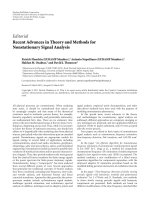
The matching constraints can be combined under different strategies, figure 1 displays a tree
with three branches (A,B and C). Each branch represents a path where the matching
constraints are applied in a different way.
As one can see, given a pair of stereoscopic images the epipolar and similarity constraints
are always applied and then depending on some factors, explained below, one can choose
one of the three alternatives, i.e. branch A, B or C. All paths end with the computation of a
disparity map, in the path A this map is a refined version of the one previously obtained
after the application of the smoothness constraint. This combination is more suitable if an
area-based strategy is being used because pixels are the most flexible features for
smoothness. Nevertheless, following the path A, we could use feature-based approaches,
such as edge-segments or regions, for computing the first disparity map. On the contrary,
branch B is more suitable when regions are used as features because it does not include the
smoothness constraint. Indeed, this constraint assumes similar disparities for entities which
are spatially near among them, but the regions could belong to different objects in the scene
and these objects do not necessarily present similar disparities. Finally, branch C could be
considered as a mixed approach where area-based or feature-based could be used, although
in this last case perhaps excluding regions. The system’s geometry which is determinant for
defining the epipolar constraint does not affect the choice of a given branch.
Combining Stereovision Matching Constraints for Solving the Correspondence Problem

91
In summary, following the branch A in section 3, we describe a first procedure based on edge-
segments as features under a conventional stereovision system and compute the first disparity
map. A second procedure is described for an omni-directional stereovision system under an
area-based approach (pixels) where a refined disparity map is finally obtained. Following the
branch B, section 4, we describe a procedure for matching regions as features from an omni-
directional stereovision system. Finally, following the branch C, section 5, the procedure
described uses again edge-segments as features in a conventional stereovision system.

pair of

stereoscopic
images
Epipolar
Similarity
uniqueness
ordering
smoothness
disparity
map
smoothness
disparity
map
refined
disparity
map
ordering
uniqueness
disparity
map
uniqueness
ABC

Fig. 1. Three different strategies for combining the stereovision matching constraints
3. Branch A: edge-segment based and pixel-based approaches
As mentioned before, under the combination scheme displayed in branch A, we describe
two procedures for computing the disparity map. The first is based on edge-segments as
features under a conventional stereovision system with parallel optical axes, where only the
first disparity map is obtained. The second uses pixels as features under a fish-eye lens
based optical system, also with parallel optical axes, where the first map is later filtered and
refined by removing errors and spurious disparity values.

3.1 Edge-segments as features: conventional stereovision systems
Under this approach the stereo matching system is designed with a parallel optical axis
geometry working in the following three stages:
1. Extracting edge-segments and their attributes from the images;
2. Performing a training process, with the samples (true and false matches) which are
supplied to a classifier based on the Support Vector Machines (SVM) framework, where
an output function is estimated through a set of attributes extracted from the edge-
segments;
Advances in Theory and Applications of Stereo Vision

92
3. Performing a matching process for each new incoming pair of features. According to the
value of the estimated output function provided by the SVM, each pair of edge-
segments is classified as a true or false match.
The first segmentation stage is common for both training and matching processes. This
scheme follows the well-known SVM learning based strategy. It has been described in
Pajares & Cruz (2003). Other learning-based methods with a similar approach, but different
learning strategies can be found in Pajares & Cruz (2002) which applies the Parzen´s
window, Pajares & Cruz (2001) which uses the ADALINE neural network, Pajares & Cruz
(2000) based on a fuzzy clustering strategy, Pajares & Cruz (1999) where the Hebbian
learning is applied and the Self-organizing framework in Pajares et al. (1998a).
Figure 2 dispalys a mapping of edge segments (u,v,h,i,c,z,k,j,s,q) as features for matching
under a conventional stereovision system with parallel optical axes and the cameras
horizontally aligned. With this geometry, the epipolar lines are horizontal crossing the left
(LI) and right (RI) images. This figure contains details about the overlapping concept firstly
introduced in Medioni & Nevatia (1985). Two segments, one in LI and the second in RI,
overlap if by sliding one of them following the epipolar line they intersect. By example, u
overlaps with c, z, s and q, but segment v does not overlap with s. Moreover, Figure 2 contains
two windows, w(i) and w(j) for applying a neighbourhood criterion, described in section
5.2.1, for mapping the smootheness constraint.

RI
u
no
overlapping
overlapping
s
q
Epipolar line
c
z
v
i
j
LI
h
k
2maxd
i
h
2maxd
w(j)
w(i)
x x
y
y
x
u
x
z

Fig. 2. Left (LI) and right (RI) images based on a conventional stereovision system with
parallel optical axes geometry and perspective projection with edge-segments as features.
3.1.1 Feature and attribute extraction
This is the first stage of the proposed approach. The contour edge pixels in both images are
extracted using the Laplacian of the Gaussian filter in accordance with the zero-crossing
criterion (Huertas & Medioni, 1986). At each zero-crossing in a given image we compute the
magnitude and the direction of the gradient vector as in Leu and Yau (1991), the Laplacian
as in Lew et al. (1994) and the variance as in Krotkov (1989). These four attributes are
computed from the gray levels of a central pixel and its eight immediate neighbors. The
gradient magnitude is obtained by taking the largest difference in gray levels of two
opposite pixels in the corresponding eight-neighbourhood of a central pixel. The gradient
direction points from the central pixel towards the pixel with the maximum absolute value
of the two opposite pixels with the largest difference. It is measured in degrees, quantified
by multiples of 45. The normalization of the gradient direction is achieved by assigning a
Combining Stereovision Matching Constraints for Solving the Correspondence Problem

93
digit from 0 to 7 to each principal direction. The Laplacian is computed by using the
corresponding Laplacian operator over the eight neighbors of the central pixel. The variance
indicates the dispersion of the nine gray level values in the eight-neighborhood of the same
central pixel. In order to avoid noise effects during edge-detection that can lead to later
mismatches in realistic images, the following two globally consistent methods are used: 1)
the edges are obtained by joining adjacent zero-crossings following the algorithm in Tanaka
& Kak (1990), in which a margin of deviation of ± 20% and ±45° is tolerated in magnitude
and direction respectively; 2) then each detected contour is approximated by a series of line
segments as in Nevatia & Babu (1980); finally, for each segment an average value for the
four attributes is obtained from all computed values of its zero-crossings. All average
attribute values are scaled, so that they fall within the same range. Each segment is
identified by its initial and final pixel coordinates, its length and its label.
Therefore, each stereo-pair of edge-segments has two associated four-dimensional vectors x

l

and x
r
, where the components are the attribute values and the sub-indices l and r denote
features belonging to the left and right images respectively. A four-dimensional difference
vector of the attributes x = {x
m
, x
d
, x
p
, x
v
} is obtained from x
l
and x
r
, whose components are
the corresponding differences for the module of the gradient vector, the direction of the
gradient vector, the Laplacian and the variance respectively.
3.1.2 Training process: the support vector machines classifier
The SVM classifier is based on the observation of a set X of n pattern samples to classify
them as true or false matches, i.e. the stereovision matching is mapped as the well-known
two classification problem. The outputs of the system are two symbolic values y ∈ {+1,–1}
corresponding each to one of the classes. So, y = +1 and y = –1 are with the class of true and
false matches respectively.
The finite sample (training) set is denoted by:
(
)

,y , =1, ,n
ii
ix , where each x
i
vector
denotes a training element and
{
}
1, 1
i
y ∈+ − the class it belongs to. In our problem x
i
is as
before the 4-dimensional difference vector.
The goal of SVM is to find, from the information stored in the training sample set, a decision
function capable of separating the data into two groups. The technique is based on the idea
of mapping the input vectors into a high-dimensional feature space using nonlinear
transformation functions. In the feature space a separating hyperplane (a linear function of
the attribute variables) is constructed (Vapnik 2000; Cherkassky & Mulier 1998). The SVM
decision function has the following general form

i
1
()= ( ,)
n
ii
i
f α yH
=
∑

xxx (1)
The equation (1) establishes a representation of the decision function f(x) as a linear
combination of kernels centred in each data point. A common kernel is the Gaussian Radial
Basis
2
(,)=exp- -H σ
⎧
⎫
⎨
⎬
⎩⎭
xy xy which is used in Pajares & Cruz (2003) where
σ
defines the
width of the kernel and was set to 3.0 after different experiments.
The parameters
,
i
i = 1, n
α
, in equation (1) are the solution for the following quadratic
optimisation problem consisting in the maximization of the functional in equation (2)
Advances in Theory and Applications of Stereo Vision

94
()
1,1
1
Q( ) = ,
2

nn
ii
j
i
j
i
j
iij
α yyH
ααα
==
−
∑∑
xx
subject to
1
00, ,
n
ii i
i
c
y
i = 1, ,n
n
αα
=
=≤≤
∑

(2)

and given the training data
(
)
ii
,
y
, i = 1, ,nx , the inner product kernel H, and the
regularization parameter
c. As stated in Cherkassky & Mulier (1998), at present, there is not
a well-developed theory on how to select the best
c, although in several applications it is set
to a large fixed constant value, such as 2000, which is used in Pajares & Cruz (2003).
The data points
x
i
associated with the nonzero
α
i
are called support vectors. Once the support
vectors have been determined, the SVM decision function has the form,

support vectors
(,)
ii i i
f( ) = y H
α
∑
xxy (3)
3.1.3 Matching process: epipolar, similarity and uniqueness constraints
Now, given a new pair of edge-segments the goal is to determine if they represent a true or

false match. Only those pairs fulfilling the overlapping concept, section 3.1, are considered.
This represents the mapping of the
epipolar constraint. The pair of segments is represented
by its attribute vector
x, therefore through the function estimated in equation (3), we
compute the scalar output
f(x) whose polarity, sign of f(x), determines the class membership,
i.e. if
x represents a true or false match for the incoming pair of edge segments. This is the
mapping of the
similarity constraint.
During the decision process there are unambiguous and ambiguous pairs of features,
depending on whether a given left image segment corresponds to one and only one, or
several right image segments, respectively based only on the polarity of
f(x). In any case, the
decision about the correct match is made by choosing the pair with the greater magnitude
f(x) when ambiguity. Because, f(x) ranges in [-1, +1] we only consider pairs with a certain
guarantee of correspondence, this means that only pairs with positive values of
f(x) are
potential candidates. Therefore, the
uniqueness constraint is formulated based on the
following decision rule: if the sign of
f(x) is positive and its value is the greatest among the
ambiguous pairs, it is chosen as a correct match, otherwise it is a false correspondence.
Figure 3 displays a pair of stereo images, which is a representative pair of the 70 pairs used
for testing in Pajares & Cruz (2003), where (
a) and (b) are respectively the left and right

(a) (b) (c)

(
d)
Fig. 3. (
a)-(b) original left and right stereo images acquired in an indoor environment; (c)-(d)
labeled left and right edge-segments extracted from the original images.
Combining Stereovision Matching Constraints for Solving the Correspondence Problem

95
images of the stereo pair. In (c) and (d) are represented the edge segments extracted
following the procedure described in section 3.1.1. Details about the experiments are
provided in Pajares & Cruz (2003), where on average the percentage of successes overpasses
the 94%. The matching between these edge segments determines the disparity map, as one
can see this map is sparse because only edges are considered.
3.2 Pixels as features: fish-eye based systems
Following the branch A, Figure 1, we again combine the epipolar, similarity and uniqueness
constraints obtaining a first disparity map. The difference with respect the method described
in section 3.1 is twofold: (
a) here the pixels are used as features, instead of edge segments; (b)
the disparity map is later refined by applying the smoothness constraint.
Additionally, the stereovision is based on cameras equipped with fish eye lenses. This
affects mainly the epipolar constraint, which is considered in section 3.2.1. Following the full
branch in figure 1, we give details about how the stereovision matching constraints are
applied under this approach. This method is described in Herrera (2010). Figure 4 displays a
pair of stereovision images captured with fish eye lenses. The method proposed here is
based on the work of Herrera et al. (2009
a) and was intended as a previous stage for forest
inventories, where the estimation of wood or the growth are some of the inventory variables
to be computed.

Fig. 4. Original stereovision images acquired with fish-eye lenses from a forest environment.
3.2.1 Epipolar constraint: system geometry
Figure 5 displays the stereo vision system geometry (Abraham & Förstner, 2005). The 3D
object point
P with world coordinates with respect to the systems (X
1
, Y
1
, Z
1
) and (X
2
, Y
2
, Z
2
)
is imaged as (
x
i1
, y
i1
) and (x
i2
, y
i2
) in image-1 (left) and image-2 (right) respectively in
coordinates of the image system;
a
1

and a
2
are the angles of incidence of the rays from P; y
12

is the baseline measuring the distance between the optical axes in both cameras along the
y-
axes;
r is the distance between an image point and the optical axis; R is the image radius,
identical in both images.
According to Schwalbe (2005), the following geometrical relations can be established,

22
11
ii
rx
y
=+;
1
2
r
α
R
π
=
;
(
)
1
11

ii
t
gy
x
β
−
= (4)
Now the problem is that the 3D world coordinates (
X
1
, Y
1
, Z
1
) are unknown. They can be
estimated by varying the distance
d as follows,

1
cos ;Xd
β
=

1
sin ;Yd
β
=

22
111 1

tanZXY
α
=+ (5)
Advances in Theory and Applications of Stereo Vision

96
From (4) we transform the world coordinates in the system O
1
X
1
Y
1
Z
1
to the world
coordinates in the system
O
2
X
2
Y
2
Z
2
taking into account the baseline as follows,

21
;XX=
2112
;YYy=+

21
ZZ
=
(6)
Assuming no lenses radial distortion, we can find the imaged coordinates of the 3D point in
image-2 as in Schwalbe (2005),

(
)
()
(
)
()
22 22
22
22
22
22 22
2 arctan 2 arctan
;
11
ii
RXYZ RXYZ
xy
YX XY
ππ
++
==
++
(7)

Because of the system geometry, the epipolar lines are not concentric circumferences and
this fact is considered for matching. Figure 6 displays four epipolar lines, in the third
quadrant of the right image, they have been generated by the four pixels located at the
positions marked with the squares, which are their equivalent locations in the left image.

image-1
image-2
1
α
2
α
P
(X
1
, Y
1
, Z
1
)
(X
2
, Y
2
, Z
2
)
X
2
O
2

Z
2
Y
2
X
1
O
1
Z
1
Y
1
x
i1
y
i1
(x
i1,
y
i1
)
(x
i2,
y
i2
)
y
12
x
i2

y
i2
r
R
R
β
β
d

Fig. 5. Geometric projections and relations for the fish-eye based stereo vision system.
Using only a camera, we capture a unique image and each 3D point belonging to the
line
1
OP, is imaged in
11
(,)
ii
xy . So, the 3D coordinates with a unique camera cannot be
obtained. When we try to match the imaged point
11
(,)
ii
xy into the image-2 we follow the
epipolar line, i.e. the projection of
1
OPover the image-2. This is equivalent to vary the
parameter d in the 3-D space. So, given the imaged point
11
(,)
ii

xy in the image-1 and
following the epipolar line, we obtain a list of m potential corresponding candidates
Combining Stereovision Matching Constraints for Solving the Correspondence Problem

97
represented by
22
(,)
ii
xy in the image-2. The best match is associated to a distance d for the
3D point in the scene, which is computed from the stereo vision system. Hence, for each d
we obtain a specific
22
(,)
ii
xy , so that when it is matched with
11
(,)
ii
xy d is the distance for
the point P. Different measures of distances during different time intervals (years) for
specific points in the trunks, such as the ends or the width of the trunk measured at the
same height, allow determining the evolution of the tree and consequently its state of
growth and also the volume of wood, which are as mentioned before inventory variables.
This requires that the stereovision system is placed at the same position in the 3D scene and
also with the same camera orientation (left camera North and right camera South).


Fig. 6. Epipolar lines in the right image generated from the locations in the left image.
3.2.2 Similarity constraint: attributes or properties

Each pixel l in the left image is characterized by its attributes; one of such attributes is
denoted as A
l
. In the same way, each candidate i in the list of m candidates is described by
identical attributes, A
i
. So, we can compute differences between attributes of the same type
A, obtaining a similarity measure for each one as follows,

()
1
1 ; i 1, ,
iA l i
sAA m
−
=+ − =
(8)
[
]
0,1 ,
iA
s ∈ 0
iA
s = if the difference between attributes is large enough (minimum similarity),
otherwise if they are equal,
1
iA
s
=
and maximum similarity is obtained.

We use the following six attributes for describing each pixel: a) correlation; b) texture; c)
colour; d) gradient magnitude; e) gradient direction and f) Laplacian. Both first ones are
area-based computed on a 3 3
×
neighbourhood around each pixel through the correlation
coefficient (Barnea & Silverman, 1972 ; Koschan & Abidi, 2008; Klaus et al., 2006) and
standard deviation (Pajares & Cruz, 2007) respectively. The four remaining ones are
considered as feature-based (Lew et al., 1994). The colour involves the three red-green-blue
spectral components (R,G,B) and the absolute value in the equation (8) is extended as the
sum of absolute differences as
,
li l i
H
AA HH−= −
∑
H = R,G,B. It is a similarity
measurement for colour images (Koschan & Abidi, 2008), used satisfactorily in Klaus et al.
(2006) for stereovision matching. Gradient (magnitude and direction) and Laplacian are
computed by applying the first and second derivatives respectively (Pajares & Cruz, 2007)
over the intensity image after its transformation from the RGB plane to the HSI (hue,
saturation, intensity) one. The gradient magnitude has been used in Lew et al. (1994) and
Klaus et al. (2006) and the direction in Lew et al. (1994). Both, colour and gradient
magnitude have been linearly combined in Klaus et al. (2006) producing satisfactory results
as compared with the Middlebury test bed (Scharstein & Szeliski, 2002). The coefficients
Advances in Theory and Applications of Stereo Vision

98
involved in the linear combination are computed by testing reliable correspondences in a set
of experiments carried out during a previous stage.
Given a pixel in the left image and the set of

m candidates in the right one, we compute the
following similarity measures for each attribute
A: s
ia
(correlation), s
ib
(colour), s
ic
(texture),
s
id
(gradient magnitude), s
ie
(gradient direction) and s
if
(Laplacian). The identifiers in the
sub-indices identify the attributes according to these assignments. The attributes are the six
ones described above, i.e.
{
}
,,,,,abcde
f
Ω≡ associated to correlation, texture, colour,
gradient magnitude, gradient direction and Laplacian.
3.2.3 Uniqueness constraint: Dempster-Shafer theory
Based on the conclusions reported in Klaus et al. (2006), the combination of attributes
appears as a suitable approach. The Dempster-Shafer theory owes its name to the works by
the both authors in Dempster (1968) and Shafer (1976) and can cope specifically with the
combination of attributes because they are specifically designed for classifier combination
Kuncheva (2004). With a little adjusting they can be used for combining attributes in

stereovision matching. They allow making a decision about a unique candidate (uniqueness
constraint). Now we must match each pixel
l in the left image with the best of the m
potential candidates.
The Dempster-Shafer theory as it is applied in our stereovision matching approach is as
follows (Kuncheva, 2004):
1.
A pixel l is to be matched either correctly or incorrectly. Hence, we identify two classes,
which are the class of true matches,
w
1,
and the class of false matches, w
2
. Given a set of
samples from both classes, we compute the similarities of the matches belonging to each
class according to (8) and build a 6-dimensional mean vector, where its components are
the mean values of their similarities, i.e.
T
,,,,,
jjajbjcjdjejf
ssssss
⎡
⎤
=
⎣
⎦
v
;
1
v and

2
v are the
mean for
w
1
and w
2
respectively; T denotes transpose. This is carried out during a
previous phase, equivalent to the training one in classification problems and the one in
section 3.1.2.
2.
Given a candidate i from the list of m candidates for l, we compute the 6-dimensional
vector
x
i
, where its components are the similarity values obtained according to (8)
between
l and i, i.e.
T
,,,,,
iiaibicidieif
ssssss
⎡
⎤
=
⎣
⎦
x
. Then we calculate the proximity Φ
between each component in

x
i
and each component in
j
v based on the Euclidean
norm
⋅
, equation (9).

()
(
)
()
1
2
1
2
2
1
1
1
iA jA
jA i
iA kA
k
ss
ss
−
−
=

+−
Φ=
+−
∑
x
where
A
∈
Ω (9)
3.
For every class w
j
and for every candidate i, we calculate the belief degrees,

()
(
)
(
)
(
)
() ()
()
1
111
jA i kA i
kj
i
j
jA i kA i

kj
bA
≠
≠
Φ
−Φ
=
⎡
⎤
−Φ − −Φ
⎣
⎦
∏
∏
xx
xx
; j = 1,2 (10)
4.
The final degree of support that candidate i, represented by
i
x , receives for each class
w
j
taking into account that its match is l is given in equation (11)
Combining Stereovision Matching Constraints for Solving the Correspondence Problem

99

(
)

(
)
i
ji j
A
bA
μ
∈Ω
=
∏
x (11)
5.
We chose as the best match for l, the candidate i with the maximum support received
for the class of true matches (
w
1
), i.e.
(
)
{
}
1
max
i
i
μ
x but only if it is greater than a
threshold, which can be fixed to 0.5, as in Herrera et al. (2009
a).
Other approaches based on the combination of attributes have been applied in Herrera et al.,

(2009
b,c) where the Choquet, Sugeno and a Fuzzy multicriteria decision making methods
are respectively used for applying the uniqueness constraint.
3.2.4 Smoothness constraint: mean filtering
We have available a first disparity map after applying the above three constraints: epipolar,
similarity and uniqueness.
The disparity map contains pixels which have been erroneously classified either as true or
false matches. Based on the obvious assumption that the structures in the 3-D scene are
spatially preserved in the 2-D images we consider that if a pixel with a disparity value
different from those values on its neighbourhood, such value must be changed toward the
disparities of the pixels which are surrounding it. This is an obvious interpretation of the
smoothness constraint. Indeed, if a point and its neighbours belong to a region in the 3-D
space, all are probably placed at a given distance from the stereovision system, this spatial
region is mapped as a 2-D region in the images and the disparities still preserve similar
values. A simple statistical averaging filter has the ability for changing erroneous or
spurious disparity values of a pixel with respect its neighbours. This technique is used in
Lankton (2010) which implements the method described in Klaus et al. (2006). Other
statistical filters could be used such as the median or the mode.
In Herrera (2010) is reported that the errors obtained without smoothing are about the 11%
and after the filtering the error decreases until the 8% on average. Figure 7 displays the
disparity maps obtained without and with smoothing. The colour bar represents the
disparity levels in sexagesimal degrees considering a circumference of 360º. The maximum
disparity value found in the twenty pairs of stereovision images used is 8º, therefore the
colour bar ranges from 0º to 8º.


(
a)

(

b)

(
c)
Fig. 7. Disparity maps (a) without smoothing and (b) with smoothing; (c) colour bar
representing the disparity levels in sexagesimal degrees.
Advances in Theory and Applications of Stereo Vision

100
4. Branch B: regions based
Now we describe the mapping of the matching constraints in the branch B, figure 1, i.e.
epipolar, similarity, ordering and uniqueness. Under this feature-based approach, the
features are regions. The stereovision system is also equipped with fish eye lenses obtaining
omnidirectional images, as the ones in figure 4. Figure 8 displays a pair of such stereo
images. As we can see, the images display similar geometry but different types of forest
environments, i.e. pines and oaks respectively. The main goal on the images in figure 8 is the
correspondence between the trunks of the trees for forest inventories because they
concentrate the greatest volume of wood and determines the growth stage of the trees,
which are important variables for inventories, as mentioned before. Therefore, this is a clear
example where the type of scene is decisive for choosing one or another strategy. So, the
strategy here differs from the one described in section 3.2, although the same final goal
(inventories) is pursued. The trunks are the regions to be matched due to its appearance.
Therefore, under this approach, an important issue concerning the stereovision matching is
the regions
segmentation, including the identification and extraction of properties, which are
used for matching. In section 4.1 we describe the segmentation process and in section 4.2 the
correspondence process, describing how the matching constraints are applied during the
correspondence process. This procedure can be found exhaustively described in Herrera et
al. (2009
d).

(
a)

(
b)
Fig. 8. Original stereo images captured in an outdoor forest environment.
4.1 Segmentation process
This process is focused on the isolation of the trunks. As we can see from figure 8, the trunks
(dark) and the sky (clear) display high contrast in a broad area in the inner part of the image,
but in the outer part they get confused with the grass in the soil. The procedure exploits the
high contrast and takes into account the last observation. By applying the following steps in
a sequential order the trunks are conveniently extrated:
1.
Valid image: the central part of the image is the one to be processed, the Charge Coupled
Device of the cameras has 1616
×
1616 pixels in width and height dimensions
respectively. The centre is located in the coordinates (808, 808). The radius R of the valid
image is 808 pixels.
2.
Detecting thin branches: thin branches are not significant for forest inventories, but they
are highly harmful from the point of view of segmentation; this is because most of these
thin branches belonging to different trees appear overlapped among them. With such
purpose we compute the standard deviation at pixel-level (Pajares & Cruz, 2007) with a
Combining Stereovision Matching Constraints for Solving the Correspondence Problem

101
window of size 5x5. Considering this window, a pixel belonging to a thin branch

fullfills the following conditions: a) displays a low intensity value, as it belongs to the
tree; b) must be surrounded by pixels with high intensity values, belonging to the sky,
this means that in the window appear pixels of this class at least in two opposite sides,
i.e. left and right or up and bottom; c) the standard deviation computed through this
window is greater than a threshold set to a value of twenty five in our experiments after
several trial and error tests, which verifies the high variability in the contrast.
3.
Concentric circumferences: we draw concentric circumferences starting with a radius r of
250 pixels from the centre, with increases of 50 pixels until r = R. We trace the intensity
profile for each circunference until a profile displays large dark areas. This means that
we have already reached the area where the trunks and soil get confused. The other
circunferences display alternative dark and clear levels, these last circumferences are
identified as type 1 and the remainder ones as type 2.
4.
Putting seeds in the trunks: given a profile of type 1, we consider a pixel in each dark
region as a seed and compute the average intensity value and standard deviation of the
dark region associated to the seed. Only dark regions with more than T
1
=10 pixels in
the profile and with intensity values below T
2
=75 are retained. Considering the outer
circumference of type 1, identified as c
i
we select only dark regions whose intersection
with this circumference gives a line with a number of pixels lower than T
3
=120. The
maximum value of all lines of intersection is
max 3

.
i
tT< Then for the next circumference
towards the centre of the image, c
i+1,

3
T is now set to
max
i
t , which is the value used when
the next circumference is processed and so on until the inner circumference of type 1 is
reached. This is justified because the thickness of the trunks always diminishes towards
the centre.
5.
Region growing: this process is based on the procedure described in Gonzalez & Woods
(2008), we start in the outer circumference of type 1 by selecting the seed pixels
obtained in this circumference. From these seed points we append to each seed those
neighbouring pixels that have a similar intensity value than the seed. The similarity is
measured as the difference between the intensity value of the pixel under consideration
and the mean value in the zone where the seed belongs to, they do not differ more than
the standard deviation for each zone. The region growing ends when no more similar
neighbouring pixels are found for that seed between this circumference and the centre
of the image. The regions obtained are labelled following the procedure described in
Haralick & Shapiro (1992).
6.
Estimation: for each labelled region we have available its orientation towards the centre
of the image and also its decreasing ratio. This allows to estimate the part of the trunk
confused with the soil. So, after this operation we obtain new enlarged regions
representing the full trunks. These regions are finally re-labelled and for each region we

extract the following attributes: area (number of pixels), centroid (xy-averaged pixel
positions in the region), angles in degrees of each centroid and the seven Hu invariant
moments (Pajares & Cruz, 2007; Gonzalez and Woods, 2008).
4.2 Matching process
Once the regions and their attributes are extracted according to the above procedure, we are
ready to apply the stereovision matching constraints in figure 1, branch B, i.e. epipolar,
similarity, ordering and uniqueness.
Advances in Theory and Applications of Stereo Vision

102
4.2.1 Epipolar constraint
As mentioned before, the images in figure 9 are captured with fish eye lenses, therefore the
epipolar lines are defined according to equations (4) to (7). So, given a region in an image
with its centroid, we search for its potential matched region following the epipolar lines and
looking for regions whose centroids fall in or near the corresponding epipolar line generated
by the first centroid in the other image of the stereoscopic pair. This idea is illustrated in
figure 9, given a red square in the image (a), following the epipolar line towards the south
direction we will find the corresponding matching, Figure 9(b). This implies that given a
centroid of a region in the left image its corresponding matching in the right image will be
probably in the epipolar line.
Because the sensor could introduce errors due to wrong calibration of the cameras, we have
considered an offset out of the epipolar lines quantified as 10 pixels in distance. Moreover,
in the epipolar line, the corresponding centroids are separated a certain angle, as we can see
in Figure 9(b) expressed by the red and blue squares. After experimentation with the set of
images tested, the maximum separation found in degrees has been quantified in 22º, i.e. this
determines the limit on the disparity.


(
a)

(
b)
Fig. 9. Original stereo images captured with a fish eye lens in an outdoor forest
environment.
4.2.2 Similarity constraint
All regions with centroids fulfilling the similarity constraint are considered as candidates for
matching. We build a list of such candidate regions according to the similarities based on
their areas and the seven Hu’s invariant moments. So, we have eight similarity
measurements, which are mapped to range in the interval [0,1]. The similarities are
stablished as differences in the absolute value between attributes. All regions with a number
of similarities greater than four and each one less than a threshold of 0.2, are considered as
candidates for matching. This threshold is fixed to this relative low value in order to
guarantee a strong similarity, taking into account that the most favourable value is zero and
the most unfavourable is +1.
4.2.3 Ordering and uniqueness constraints
The ordering constraint assumes that the relative position between two regions in an image
is preserved in the other one for the corresponding matches. The application of this
constraint is limited to regions with similar heights and areas in the same image and also if
the areas overpass a threshold T
4
set to 6400 in this work. This tries to avoid violations of
Combining Stereovision Matching Constraints for Solving the Correspondence Problem

103
this constraint based on closeness and remoteness relations of the trunks with respect the
sensor in the 3D scene.
If after applying the similarity constraint still remain ambiguities because different pairs of
regions still involve the same region, the application of the ordering constraint could
remove these possible ambiguities. This implies the implicit application of the uniqueness

constraint. Nevertheless, if still ambiguities persist, we strictly select the most similar pairs
in application of the similarity constraint until all ambiguities are resolved.
Figure 10 displays the regions extracted by the segmentation process. Each region appears
with a unique label. The number near of the regions identifies each label. This number is
represented as a color in a scale ranging from 1 to 14, where 1 is blue and 14 orange. This
representation is only for a best visualization of the regions.


(
a)

(
b)
Fig. 10. Labelled regions: (a) left image, (b) right image. Each region appears identified by a
unique number.
From Figure 10, we can see how the segmented regions come from the trunks in Figure 4,
even trunks displaying small areas. The proposed approach over the set of 20 stereo pairs of
images analyzed has achieved a performance of 88.4% of successes.
5. Branch C: edge segments based
This approach follows the branch C in figure 1, i. e. here epipolar, similarity, smoothness
ordering and uniqueness are the constraints to be applied. The features are edge segments
as the ones used in section 3.1. We extract these features and apply the two first constraints
exactly as described in such section. The full procedure is described in Pajares & Cruz
(2004). Other similar global stratetigies can be found in Pajares et al. (2000) where a Hopfield
neural network is the chosen global matching approach selected or in Pajares et al., (1998
b)
where a relaxation approach is applied. Also global strategies are applied in Ishikawa &
Geiger (2007) where an energy minimization is defined with such purpose or in Pajares &
Cruz (2006), where the fuzzy cognitive map framework is the method selected for achieving
the proposed globality.

5.1 Epipolar and similarity constraints
Consequently, after applying the training process described in section 3.1.2, we obtain the
decision function in equation (3). Given a pair of stereo images as those displayed in figure
3(
a) and (b) we obtain for each pair of edge segments the corresponding attribute difference
vector,
x
, as described in section 3.1.1. Once this vector is computed, we could take a
decision about tha matching of the pair of edge segments that it represents as in section
Advances in Theory and Applications of Stereo Vision

104
3.1.3. Nevertheless, in order to embed the similarity in the global matching process
described later, we map the value provided by the decision function to range in the
continuous interval [-1,+1] as a similarity measurement between features as follows,

()
2
() 1
1exp ()
ij
s
af
=
−
+−
x
x
(12)
where, in order to avoid severe bias, the parameter

a is estimated experimentally, verifying
that a value of 0.2 suffices for the type of images analysed. Implicitly, at this stage we have
already applied the epipolar and similarity constraints.
5.2 Simulated annealing: a global matching strategy
In order to formulate the Simulated Annealing (SA) we build a network of nodes, where
each pair of edge-segments to be matched creates a node with its own state, which
determines the strength of the correspondence. Through the equation (12), the nodes are
loaded with an initial state, which is updated through the SA optimization process. The
correspondences are established based on the final values of the states.
The goal of the optimization process is to increase the consistency of a given pair of edge
segments among three constraints (smoothness, ordering and epipolar) so that the state of a
node representing a correct match can be increased and the state of any incorrect match can
be decreased during the optimization process. Suppose the network with
N nodes. The
simulated annealing optimization problem is: modify the state values
s
ij
so as to minimize
the energy,

()( )
11
1
=-
2
NN
i
j
hk i
j

hk
ij hk
Ewss
==
∑∑
(13)
where
()( )i
j
hk
w is a symmetric weight interconnecting two nodes (i,j) and (h,k). We require the
self-feedback terms to vanish (i.e.
()()
0
ij ij
w
=
) because the nonzero merely add an
unimportant constant to
E, independent of the s
ij
. The optimization task is to find the
network with the most stable configuration, the one with lowest energy. The energy
function is built so that it embeds three stereovision constraints:
smoothness, ordering and
epipolar, this last once again considered. Therefore, we look for a compatibility coefficient,
which must be able to represent the consistency between the current pair of edge segments
under correspondence and the pairs of edge segments in a given neighborhood. The
compatibility coefficient makes global consistency between neighbors pairs of edge
segments based on such constraints.

5.2.1 Mapping the smoothness constraint
The smoothness constraint assumes that neighboring edge segments have similar
disparities, except at a few depth discontinuities (Medioni & Nevatia, 1985). Generally,
when the smoothness constraint is applied, it is assumed there is a bound on the disparity
range allowed for any given segment. We denote this limit as
maxd, in the set of images
tested, a value of 15 suffices, (see figure 2). According to the procedure described in Medioni
& Nevatia (1985), for each edge segment "
i" in the left image we define a window w(i) in the
right image in which corresponding segments from the right image must lie and, similarly,
for each segment "
j" in the right image, we define a window w(j) in the left image in which
Combining Stereovision Matching Constraints for Solving the Correspondence Problem

105
corresponding edge segments from the left image must lie. It is said that "a segment h must
lie" if at least the 30% of the length of the segment "
h" is contained in the corresponding
window. The shape of this window is a parallelogram, one side is "
i", for left to right match,
and the other a horizontal vector of length
2.maxd. The smoothness constraint implies that
"
i" in w(j) assumes "j" in w(i).
Now, given “
i” and “h” in w(j) and “j” and “k” in w(i) where “i” matches with “j” and “h”
with “
k” the differential disparity |d
ij
- d

hk
|, measures how close the disparity between edge
segments “
i” and “j” denoted as d
ij
is to the disparity d
hk
between edge segments “h” and
“
k”. The disparity between edge segments is the average of the disparity between the two
edge segments along the length they overlap. This differential disparity criterion is used in
Medioni & Nevatia (1985), Ruichek & Postaire (1996), Pajares et al., (1998
b, 2000), Pajares &
Cruz (2004) or Nasrabadi & Choo (1992) among others. We define a compatibility coefficient
derived from Ruichek & Postaire (1996) and Nasrabadi & Choo (1992) given by the
following expression,

()
()( )
2
()= -1
1+exp γ ()-1
ij hk
cD
DmD
⎡
⎤
⎣
⎦
(14)

where
=
i
j
hk
Dd d− , m(D) denotes the average of all values D in the pair of stereo images (LI
and
LR, see figure 2) under processing. The slope of the compatibility coefficient in (14) is
expressed by
γ
and varies for each pair of stereo images. To determine
γ
, it is assumed that
the probability distribution function of
D is Gaussian with average m(D) and standard
deviation
()σ D , i.e.
()
1
()( )
() 1+expγ ()-1
ij hk
pD D mD
−
⎡
⎤
⎡
⎤
=
⎣

⎦
⎣
⎦
.
Under this assumption and following Kim et al. (1997) and Kreszig (1983), to set the
possibility value to 0.1 when the value of cumulative distribution function is 0.9,
γ
value is
calculated by
(
)
(
)
(
)
= ln9 ( ) 1.282 ( )γ mD σ D . In our experiments, typical values of
γ
, m(D)
and
()σ D are about 6, 9 and 2 respectively. So, values of D near 0 should give high values in
the compatibility coefficient
()( )
() +1
ij hk
c
⋅
≈ , but near 25 they give low values,
()( )
() 1
ij hk

c ⋅≈−
and intermediate values should give values near zero, as expected. Note that
()( )
()
ij hk
c ⋅
ranges in (
−1,1). This means that a compatibility coefficient of +1 is obtained for a good
consistency between two nodes (
i,j) and (h,k) (i.e. D = 0) and a compatibility of −1 for a bad
consistency between these nodes (i.e.
D>>0).
The energy function embedding the smoothness constraint must be minimum when
D = 0
(i.e. corresponding to a high compatibility coefficient value) and high states values. We
define an energy function assuming the above as follows,

11
NN
(i
j
)(hk) i
j
hk
ij hk
A
E=- c ss
s
2
==

∑∑
(15)
where
A is a positive constant to be defined later.
5.2.2 Mapping the ordering constraint
We define the ordering coefficient
()( )i
j
hk
O for the edge-segments according to (16), which
measures the relative average position of edge segments
“i” and “h” in the left image with
respect to
“j” and “k” in the right image, it ranges from 0 to 1.
Advances in Theory and Applications of Stereo Vision

106

(ij)(hk) (ij)(hk) (ij)(hk) i h j k
N
1 if r > 0
1
O = o where o = S(x x ) - S(x - x ) and S(r) =
0 otherwise
N
⎧
⎨
⎩
∑
(16)

We trace
S scanlines (in our experiments four are sufficient) along the common overlapping
length, each scanline produces a set of four intersection points (
i
S
and h
S
in LI and j
S
and k
S
in
the
RI) with the four edge-segments. Hence, the lower-case o
ijhk
can be computed as in
Ruichek & Postaire (1996) considering the above four edge points, and it takes 0 and 1 as
two discrete values.
As
()( )
()
ij hk
c ⋅ ranges in [−1,+1], in order to achieve similar contributions, we re-scale the
()( )i
j
hk
O

values to [−1,+1] as follows:
()( )

()( )
=2 -1
ij hk
ij hk
OO .
To satisfy the ordering constraint, the energy function should have its minimum value when
the nodes constituting each pair of nodes, for which the corresponding edges do not satisfy
the ordering constraint, have high states values simultaneously. The energy function could
be written as follows,

()( )
NN
oi
j
hk i
j
hk
ij=1 hk=1
B
EOss
2
=
∑∑
(17)
where
B is a positive constant to be defined later.
5.2.3 Mapping the epipolar constraint
Although this constraint has been applied previously during the matching based on the
similarity, now it is again mapped under the global point of view based on the overlapping
concept, section 3.1. Based on the Figure 2, the overlap rate between edge segments (

u,z), a
uz

is defined as the percentage of coincidence, ranging in [0,1], when two segments
u and z
overlap, and it is computed taken into account the common overlap length
l
c
defined by c
and the two lengths for the involved edge segments
l
u
and l
z
respectively. All lengths are
measured in pixels.

()
=2
uz c u z
α ll+l (18)
Based on the overlapping concept, we compute the overlapping coefficient as follows,

(
)
()( )
0.5
i
j
hk i

j
hk
λ
= α + α (19)
Under the epipolar constraint we can assume that correct matches should have high overlap
rates and
()( )i
j
hk
λ for neighborhoods should be high, increasing the consistency. The
overlapping criterion is justified by the fact that the edge segments are reconstructed by
piecewise linear line segments as described in section 3.1.1. As before, we re-scale the
()( )i
j
hk
λ
values to the interval [
−1,+1] as follows:
()( ) ()( )
1
ij hk ij hk
λ =2λ
−
. The energy function should
have its minimum value when the nodes constituting each pair of nodes, for which the
corresponding edges satisfy the overlapping concept, have high
()( )i
j
hk
λ ( 1

≈
) and high states
values simultaneously. The energy could be written as

()( )
11
NN
ei
j
hk i
j
hk
ij hk
C
E=-
λ
ss
2
==
∑∑
(20)
Combining Stereovision Matching Constraints for Solving the Correspondence Problem

107
5.2.4 Deterministic simulated annealing
The total energy function can be obtained as E = E
s
+ E
o
+ E

e
. By comparison of expressions
(15), (17) and (20) and (13), by multiplying the constant term by -1, it is easy to derive the
connection weights,

(
)
()() ()() ()() ()() ()()ij hk ij hk ij hk ij hk ij hk
wAcBOC
λδ
=−+− (21)
where the delta function
()( )
1
ij hk
δ = for (i,j) = (h,k) and 0 otherwise. To ensure the
convergence to stable state, symmetrical inter-connection weights and no self-feedback are
required, i.e. we see that by setting A = B = C = 1 both conditions are fulfilled.
The simulated annealing process, was originally developed in Kirkpatrick et al. (1983) and
Kirkpatrick (1984), in this chapter we have implemented the approach described in Duda et
al. (2001) and Haykin (1994). According to Duda et al. (2001), we have chosen deterministic
simulated annealing because the stochastic one is slow. Nevertheless, the deterministic
version has been faster than the stochastic, by exactly two orders of magnitude, this agrees
with Duda et al. (2001).
In the original SA algorithm, the forces exerted by the other nodes are summed to find an
analogue value
s
ij
without the intervention of the state of the node which is being updated.
We modify this in order to include the contribution of its own state, so that the power of the

similarity constraint is considered. The temperature (
T) also plays a very important role in
the optimization process.
Let
() ()( )
()
i
j
i
j
hk hk
hk
Fws=
∑
be the force exerted on node (i,j) by the other nodes (h,k), then the
new state
s
ij
(t) is obtained by adding the fraction (,)f
⋅
⋅ to the previous one,

(
)
() ()
() () () ( 1) () () ( 1)
ij ij ij ij ij
st=
f
(F t ,T t )+ s t - = tanh F t T t + s t -

(22)
where
t represents the iteration index. The fraction (,)f
⋅
⋅ depends upon the temperature. At
high
T, the value of (,)f
⋅
⋅ is lower for a given value of the forces F. Details about the
behavior of
T are given in Duda et al. (2001). We have verified that this fraction must be
small as compared to ( - 1)
ij
st in order to avoid that the updating is controlled by this
fraction exclusively and that the similarity constraint is cancelled. Under the above
considerations and based on Starink & Backer (1995) and Hajek (1988), the following
annealing schedule suffices to obtain a global minimum:
(
)
()
0
Tt =T lo
g
t+1 , with T
0
being a
sufficiently high initial temperature. We have computed
0
T as follows (Laarhoven & Aarts,
1989): 1) we select four stereo images, previously the Support Vector Machines has been

trained and the support vectors obtained; now we compute the initial energy; 2) we choose
an initial temperature that permits about 80% of all transitions to be accepted (i.e. transitions
that decrease the energy function), and this value is changed until such percentage is
achieved; 3) we compute the
M transitions
i
ΔE and we look for a value for T for which
1
1
exp 0.8
M
i
i
E
MT
=
Δ
⎛⎞
−=
⎜⎟
⎝⎠
∑
, after rejecting the higher order terms of the Taylor expansion of the
exponential,
5
i
T= EΔ , where
⋅
is the mean value. In our experiments, we have obtained
6.10

i
EΔ= , giving
0
30.5T= (with a similar order of magnitude as that reported in Starink
& Backer (1995) and Hajek (1988)). We have also verified that a value of
t
max
= 100 suffices,
Advances in Theory and Applications of Stereo Vision

108
although the expected condition () 0, Tt t
=
→+∞ in the original algorithm is not fully
fulfilled. But this last requirement and a possible overly rapid cooling only occur when
simulated annealing is applied for achieving the solid thermal equilibrium but not in our
approach in which there is not a solid. Moreover, the above cooling scheduling is justified
by the fact that our initial state has reached a certain equilibrium as a result of the Support
Vector Machines local matching process and it is unnecessary to heat at high temperature,
hence we have a prior knowledge about the system before it is relaxed by SA.
The proposed deterministic SA algorithm derived from Duda et al. (2001) including the
modifications mentioned is summarized as follows:
1.
Initialization: t = 0,
0
(0)TT
=
, w
(ij)(hk)
as given by equation (21), s

ij
ij = 1, ,N the state
values received from the Support Vector Machines
2.
Simulated Annealing process: set t = t + 1 and np = 0
for each node (i,j) update ( )
ij
staccording to (22) and if () ( 1)
ij ij
st st
ε
−
−>then np = np +
1 when all (
i,j) nodes are updated, if np 0
≠
or
max
t<t then go to step 2, else stop.
3. Output:
i
j
s updated
np is the number of nodes for which the matching states are modified by the updating
procedure,
N is the number of nodes, T(t) is the annealing schedule,
ε
is a constant to
accelerate the convergence, set to 0.01.
5.2.5 Mapping the uniqueness constraint

This stage represents the mapping of the uniqueness constraint, which completes the set of
matching constraints used for solving our stereovision matching problem.
A left edge segment can be assigned to a unique right edge segment (unambiguous pair) or
several right edge segments (ambiguous pairs).
The decision about whether a match is correct is made by choosing the greater state value in
the network of nodes (in the unambiguous case there is only one) whenever it surpasses a
previous fixed threshold
U
1
(= 0), intermediate value for s
ij
ranging in [−1,+1]. A true match
should have
s
ij
= +1.
The ambiguities produced by broken edge segments are allowed. Therefore, we make a
provision for broken segments resulting in possible multiple correct matches. The following
pedagogical example from figure 2 clarifies this. The edge segment
u in LI matches with the
broken segment represented by
s and q in RI, but under the condition that s and q do not
overlap, that the
s and q orientations do not differ by more than U
2
(±10°) and both s
us
, s
ut
are

greater than
U
1
.
6. Conclusion
This chapter presents a survey about the application of several stereovision matching
approaches which are applied under different strategies. Three main features are used:
pixels, edge-segments and regions. The mapping of the constraints differs depending on
these features that in turn are determined depending on the type of scene. Also, a general
review is made about different strategies in conventional and fish eye based systems. These
last producing omni-directional images.
We have established the bases for extending the scheme in figure 1, if required, by
introducing more matching constraints, such as the optical flow (Kim & Yi, 2008).
Combining Stereovision Matching Constraints for Solving the Correspondence Problem

109
7. Acknowledgments
We would like to thank Dr. Fernando Montes and Isabel Cañellas from the Forest Research
Centre (CIFOR) in the National Institute for Agriculture and Food Research and Technology
(INIA) for the omnidirectional images supplied and acquired by the measurement device
with number of patent MU-200501738. The authors wish to acknowledge to the Council of
Education of the Autonomous Community of Madrid and the Social European Fund for the
research contract with the second author.
Authors thank the European Union, the European Commission and CONACYT by the
economical support received from the European Commission under grant FONCICYT 93829
and grant 245986 in the Theme NMP-2009-3.4-1 (Automation and robotics for sustainable
crop and forestry management). The content of this chapter is an exclusive responsibility of
the University Complutense and it cannot be considered that it reflects the position of the
European Union.
Finally, partial funding has also been received from DPI2009-14552-C02-01 project,

supported by the Ministry of Spain Science and Technology within the Plan Nacional de
I+D+i.
8. References
Abraham, S. & Förstner, W. (2005). Fish-eye-stereo calibration and epipolar rectification.
Photogrammetry and Remote Sensing, vol. 59, pp. 278–288.
Barnard, S. & Fishler, M. (1982). Computational Stereo.
ACM Computing Surveys, vol. 14, pp.
553-572.
Barnea, D.I. & Silverman, H.F. (1972). A class of algorithms for fast digital image
registration.
IEEE Trans. Computers, 21, 179-186.
Cherkassky, V. and Mulier, F. 1998
. Learning from Data: Concepts, Theory and Methods. Wiley,
New York.
Dempster, A.P. (1968). A generalization of Bayesian inference,
Journal of the Royal Statistical
Society
, vol. B 30, pp. 205-247.
Duda, R.O.; Hart, P.E. & Stork, D.G. (2001).
Pattern Classification, Wiley, New York.
Gonzalez, R.C. & Woods, R.E. (2008).
Digital Image Processing, Prentice-Hall: Bergen County,
NJ, USA.
Grimson, W.E.L. (1985). Computational experiments with a feature-based stereo algorithm.
IEEE Transactions on Pattern Analysis and Machine Intelligence, vol. 7, pp. 17-34.
Haralick, R.M. & Shapiro, L.G. (1992).
Computer and Robot Vision, Vols. I–II, Addison-Wesley:
Reading, MA, USA.
Hajek, B. (1988). Cooling schedules for optimal annealing.
Mathematical Operation Research,

vol. 13, pp. 311-329.
Haykin, S. (1994). Neural Networks:
A Comprehensive Foundation, Macmillan College
Publishing Company, New York.
Herrera, P.J.; Pajares, G.; Guijarro, M.; Ruz, J.J. & Cruz, J.M. (2009
a). Choquet Fuzzy Integral
applied to stereovision matching for fish-eye lenses in forest analysis, in: W. Yu and
E.N. Sanchez (Eds.),
Advances in Computational Intell., AISC 61, Springer-Verlag
Berlin Heidelberg, pp. 179–187.
Herrera, P.J.; Pajares, G.; Guijarro, M.; Ruz, J.J. & Cruz, J.M. (2009
b). Combination of
attributes in stereovision matching for fish-eye lenses in forest analysis, in: J. Blanc-
Advances in Theory and Applications of Stereo Vision

110
Talon et al. (Eds.), Advanced Concepts for Intelligent Vision Systems (ACIVS 2009),
LNCS 5807, Springer-Verlag Berlin Heidelberg, pp. 277-287.
Herrera, P.J.; Pajares, G.; Guijarro, M.; Ruz, J.J. & Cruz, J.M. (2009
c). Fuzzy Multi-Criteria
Decision Making in Stereovision Matching for Fish-Eye Lenses in Forest Analysis,
in: H. Yin and E. Corchado (Eds.),
Intelligent Data Engineering and Automated
Learning
(IDEAL 2009), Lecture Notes Computer Science vol. 5788, pp. 325-332,
Springer-Verlag Berlin Heidelberg, .
Herrera, P.J.; Pajares, G.; Guijarro; M., Ruz, J.J.; Cruz, J.M. & Montes, F., (2009
d). A Featured-
Based Strategy for Stereovision Matching in Sensors with Fish-Eye Lenses for
Forest Environments,

Sensors, vol. 9, no. 12, pp. 9468-9492.
Herrera, P.J. (2010). Correspondencia estereoscópica en imágenes obtenidas con proyección
omnidireccional para entornos forestales. PhD Dissertation (in spanish), Facultad
of Informatics. University Complutense.
Huertas, A. & Medioni, G. (1986). Detection of Intensity Changes with Subpixel Accuracy
Using Laplacian-Gaussian Masks.
IEEE Trans. Pattern Anal. Machine Intelligence, vol.
8, no. 5, pp. 651-664.
Ishikawa, H. & Geiger, D. (2007). Local Feature Selection and Global Energy Optimization in
Stereo. In :
Scene Reconstruction, Pose Estimation and Tracking, R. Stolkin (Ed.), pp.
411-429, I-Tech, ISBN: 978-3-902613-06-6, Vienna, Austria.
Kim, Y.S.; Lee, J.J. & Ha, Y.H. (1997). Stereo matching algorithm based on modified Wavelet
decomposition process.
Pattern Recognition, vol. 30, no. 6, pp. 929-952.
Kim, Y.H. & Yi, S.Y. (2008). Using Optical Flow as an Additional Constraint for Solving the
Correspondence Problem in Binocular Stereopsis. In :
Stereo Vision, Asim Bhatti
(Ed.), pp. 335-348, I-Tech, ISBN: 978-953-7619-22-0, Vienna, Austria.
Kirkpatrick, S.; Gelatt, C.D. & Vecchi, M.P. (1983). Optimization by simulated annealing,
Science, vol. 220, pp. 671-680.
Kirkpatrick, S. (1984). Optimization by simulated annealing: quantitative studies. J.
Statistical Physics, vol. 34, pp. 975-984.
Klaus, A.; Sormann, M. & Karner, K. (2006). Segmented-Based Stereo Matching Using Belief
Propagation and Self-Adapting Dissimilarity Measure, In:
Proc. of 18th Int.
Conference on Pattern Recognition
, vol. 3, pp. 15-18.
Koschan, A. & Abidi, M. (2008).
Digital Color Image Processing, Wiley.

Kreszig, E. (1983).
Advanced Engineering Mathematics, Wiley, New York.
Krotkov, E.; Henriksen, K., & Kories, R. (1990). Stereo Ranging with Verging Cameras.
IEEE
Trans. on Pattern Analysis and Machine Intelligence
, vol. 12, no. 12, pp. 1200-1205.
Kuncheva, L. (2004).
Combining Pattern Classifiers: Methods and Algorithms, Wiley.
Laarhoven, P.M.J. & Aarts, E.H.L. (1989).
Simulated Annealing: Theory and Applications,
Kluwer Academic, Holland.
Lankton, S. (2010). />disparity/ (available on-line).
Leu, J.G. & Yau, H.L. (1991). Detecting the Dislocations in Metal Crystals from Microscopic
Images.
Pattern Recognition, vol. 24, no. 1, pp. 41-56.
Lew, M.S., Huang, T.S. & Wong, K. (1994). Learning and Feature Selection in Stereo
Matching.
IEEE Trans. Pattern Anal. Machine Intell. vol. 16, no. 9, pp. 869-881.
Lopez-Malo, M.A. & Pla, F. (2000). Dealing with Segmentation Errors in Region-based
Stereo Matching,
Pattern Recognition, vol. 8, no. 33, pp. 1325-1338.
Combining Stereovision Matching Constraints for Solving the Correspondence Problem

111
McKinnon, B. & Baltes, J. (2004). Practical Region-Based Matching for Stereo Vision. In: 10th
International Workshop on Combinatinal Image Analysis
(IWCIA'04), Klette, R., Zunic,
J., (Eds.), vol. 3322, pp. 726–738,
Lecture Notes Computer Science, Springer, Berlin.
Marapane, S.B. & Trivedi, M.M. (1989). Region-based stereo analysis for robotic

applications.
IEEE Transactions on Systems, Man and Cybernetics vol. 19(6), pp. 1447-
1464.
Medioni, G. & Nevatia, R. (1985). Segment Based Stereo Matching.
Computer Vision, Graphics
and Image Processing
, vol. 31, pp. 2-18.
Nasrabadi, N.M. & Choo, C.Y. (1992). Hopfield network for stereovision correspondence.
IEEE Transactions on Neural Networks, vol. 3, pp. 123-135.
Nevatia, R. & Babu, K.R. (1980). Linear Feature Extraction and Description.
Computer Vision,
Graphics, and Image Processing
, vol. 13, pp. 257-26.
Pajares, G. & Cruz, J. M. & Aranda, J. (1998
a). Stereo Matching based on the Self-Organizing
Feature-Mapping algorithm,
Pattern Recognition Letters , vol. 19, pp. 319-330.
Pajares, G. ; Cruz, J.M. & Aranda, J. (1998
b). Relaxation by Hopfield Network in Stereo
Image Matching, Pattern Recognition, vol. 31(5), pp. 561-574.
Pajares, G. & Cruz, J. M. (1999). Stereo Matching using Hebbian learning,
IEEE Transactions
on Systems Man and Cybernetics, Part B: Cybernetics
, vol. 29, no. 4, pp. 553-559.
Pajares, G. & Cruz, J.M. (2000). A new learning strategy for stereo matching derived from a
fuzzy clustering method,
Fuzzy Sets and Systems, vol. 110, no. 3, pp. 413-427.
Pajares, G. ; Cruz, J.M. & López-Orozco, J.A. (2000). Relaxation labeling in stereo image
matching,
Pattern Recognition, vol. 33, pp. 53-68.

Pajares, G. & Cruz, J. M. (2001). Local stereovision matching through the ADALINE neural
network,
Pattern Recognition Letters, vol. 22, no. 14, pp. 1457-1473.
Pajares, G. & Cruz, J. M. (2002). The non-Parametric Parzen's window in stereovision
matching,
IEEE Transactions on Systems Man and Cybernetics, Part B: Cybernetics,
vol. 32, no. 2, pp. 225-230.
Pajares, G. & Cruz, J.M. (2003). Stereovision matching through Support Vector Machines,
Pattern Recognition Letters, vol. 24, no. 15, pp. 2575-2583.
Pajares, G. & Cruz, J. M. (2004). On combining support vector machines and simulated
annealing in stereovision matching.
IEEE Trans. Systems Man and Cybernetics, Part B,
vol. 34, no. 4, pp. 1646-1657.
Pajares, G & Cruz, J.M. (2006). Fuzzy cognitive Maps for Stereo Matching.
Pattern
Recognition
, vol 39, pp. 2101-2114.
Pajares, G. & de la Cruz, J.M. (2007).
Visión por Computador: Imágenes digitales y aplicaciones,
RA-MA.
Ruichek, Y. & Postaire, J.G. (1996). A neural network algorithm for 3-D reconstruction from
stereo pairs of linear images.
Pattern Recognition Letters, vol. 17, pp. 387-398.
Ruichek, Y.; Hariti, M. & Issa, H. (2007). Global Techniques for Edge based Stereo Matching.
In :
Scene Reconstruction, Pose Estimation and Tracking, R. Stolkin (Ed.), pp. 383-410, I-
Tech, ISBN: 978-3-902613-06-6, Vienna, Austria.
Scaramuzza, D.; Criblez, N.; Martinelli, A. & Siegwart, R. (2008). Robust Feature Extraction
and Matching for Omnidirectional Images. In:
Field and Service Robotics, Laugier, C.,

Siegwart, R., (Eds.), vol. 42, pp. 71–81, Springer, Berlin, Germany.
Advances in Theory and Applications of Stereo Vision

112
Scharstein, D. & Szeliski, R. (2002). A taxonomy and avaluation of dense two-frame stereo
correspondence algorithms,
Int. J. Computer Vision, vol. 47, no. 1-3, pp. 7–42, (2002).

Schwalbe, E. (2005). Geometric modelling and calibration of fisheye lens camera systems. In
Proc. 2nd Panoramic Photogrammetry Workshop, Int. Archives of Photogrammetry and
Remote Sensing, vol. 36, Part 5/W8.
Shafer, G. (1976).
A Mathematical Theory of Evidence. Princeton University Press.
Starink, J. P. & Backer, E. (1995). Finding Point Correspondences Using Simulated
Annealing,
Pattern Recognition, vol. 28, no. 2, pp. 231-240.
Tanaka, S. & Kak, A.C. 1990. A Rule-Based Approach to Binocular Stereopsis. In:
Analysis
and Interpretation of Range Images,
Jain, R.C. Jain, A.K. (Eds.), Chapter 2, Springer-
Verlag, Berlin.
Tang, L. ; Wu, C. & Chen, Z. (2002). Image dense matching based on region growth with
adaptive window.
Pattern Recognition Letters, vol. 23, pp. 1169-1178.
Vapnik, V.N. 2000.
The nature of Statistical Learning Theory. Springer-Verlag, New York.
Wei, Y. & Quan, L. (2004). Region-Based Progressive Stereo Matching. In:
Proc. of the IEEE
Computer Society Conference on Computer Vision and Pattern Recognition
(CVPR’04),

vol. 1. pp. 106-113.
6
A High-Precision Calibration Method for
Stereo Vision System
Chuan Zhou, Yingkui Du and Yandong Tang
State Key Laboratory of Robotics
Shenyang Institute of Automation
Chinese Academy of Sciences
P.R. China
1. Introduction
Stereo vision plays an important role in planetary exploration, for it can percept and
measure the 3-D information of the unstructured environment in a passive manner
(Goldberg et al., 2002; Olson et al., 2003; Xiong et al., 2001). It can provide consultant
support for robotics control and decision-making. So it is applied in the field of rover
navigation, real-time hazard avoidance, path programming and terrain modelling. In some
cases, one stereo-vision system must accomplish both hazard detection and accurate
localization with short baseline, i.e. 100-200mm in length. This seems to be a little
ambivalent, for hazard detection needs wide view field, while accurate localization is on the
contrary. Reconstruction precision is inverse proportion to focal length if the baseline is
fixed. So researchers have to first select a compatible view angle, which guarantees the task
workspace is within the view field. Then they must refine their camera calibration method
in order to satisfy the accuracy requirement of rover localization, navigation and task
operation.
In order to satisfy these requirements, wide angle lens is usually used. Lens distortion may
reduce the precision of localization. So distortion parameter calibration plays an important
part in such case. Moreover, calibration accuracy may also affect the complexity of the
matching process. Tsai (R, Y, Tsai, 1987) proposed a method, in which a distorted parameter
is used to describe the radial distortion of the lens. A five-parameter model is exploited to
characterize several kinds of lens distortion (Yunde et al., 2000). A more complicated model,
CAHVORE, is introduced (Gennery, 2001). Calibration becomes a nonlinear process if lens

distortion is introduced. Usually camera calibration needs two steps. The first step generates
an approximate solution using a linear technique, while the second step refines the linear
solution using a nonlinear iterative procedure. The approximate solutions provided by the
linear techniques must be good enough for the subsequent nonlinear technique to correctly
converge. After the initial value has been obtained, the precision of the final result and
convergence speed depends closely on optimization algorithm. Most of existing nonlinear
methods minimize the geometric cost function using variants of conventional optimization
techniques like gradient-descent, conjugate gradient descent Newton or Levenberg-
Marquardt (LM) method. Therefore there are some problems in these circumstances. First, it
is the commonly used cost function, reprojection error, which minimizes the distance