Automation and Robotics Part 3 pot
Bạn đang xem bản rút gọn của tài liệu. Xem và tải ngay bản đầy đủ của tài liệu tại đây (1.94 MB, 25 trang )
Automation and Robotics
44
sensor plane, as shown in Fig.1. The center of projection O
C
, also called the camera center, is
the origin of a coordinate system (CS)
{
}
ccc
ZYX
ˆ
,
ˆ
,
ˆ
in which the point
C
r
G
is defined (later
on, this system we will be referred to as the Camera CS). By using the triangle similarity rule
(confer Fig.1) one can easily see that the point
C
r
G
is mapped to the following point:
T
⎥
⎦
⎤
⎢
⎣
⎡
−−=
C
C
C
C
C
C
C
z
y
f
z
x
fr
G
that means that
T
⎥
⎥
⎦
⎤
⎢
⎢
⎣
⎡
−−=
C
C
C
C
C
C
C
z
y
f
z
x
fr
G
(1)
which describes the central projection mapping from Euclidean space R
3
to R
2
. As the
coordinate z
C
cannot be reconstructed, the depth information is lost.
Fig. 1. Right side view of the camera-lens system
The line passing through the camera center O
C
and perpendicular to the sensor plane is
called the principal axis of the camera. The point where the principal axis meets the sensor
plane is called a principal point, which is denoted in Fig. 1 as C.
The projected point
S
r
G
has negative coordinates with respect to the positive coordinates of
the point
C
r
G
due to the fact that the projection inverts the image. Let us consider, for
instance, the coordinate y
C
of the point
C
r
G
. It has a negative value in space because the axis
C
Y
ˆ
points downwards. However, after projecting it onto the sensor plane it gains a positive
value. The same concerns the coordinate x
C
. In order to omit introducing negative
coordinates to point
S
r
G
, we can rotate the image plane by 180 deg around the axes
C
X
ˆ
and
Vision Guided Robot Gripping Systems
45
C
Y
ˆ
obtaining a non-existent plane, called an imaginary sensor plane. As can be seen in Fig. 1,
the coordinates of the point
'S
r
G
directly correspond to the coordinates of point
C
r
G
, and the
projection law holds as well. In this Chapter we shall thus refer to the imaginary sensor
plane.
Consequently, the central projection can be written in terms of matrix multiplication:
⎥
⎥
⎥
⎥
⎥
⎥
⎦
⎤
⎢
⎢
⎢
⎢
⎢
⎢
⎣
⎡
⎥
⎥
⎥
⎦
⎤
⎢
⎢
⎢
⎣
⎡
=
⎥
⎥
⎥
⎥
⎥
⎥
⎦
⎤
⎢
⎢
⎢
⎢
⎢
⎢
⎣
⎡
→
⎥
⎥
⎥
⎦
⎤
⎢
⎢
⎢
⎣
⎡
1
100
00
00
1
C
C
C
C
C
C
C
C
C
C
C
C
C
C
C
z
y
z
x
f
f
z
y
f
z
x
f
z
y
x
(2)
where
⎥
⎥
⎥
⎦
⎤
⎢
⎢
⎢
⎣
⎡
=
100
00
00
c
c
f
f
M is called a camera matrix.
The pinhole camera describes the ideal projection. As we use CCD cameras with lens, the
above model is not sufficient enough for precise measurements because factors like
rectangular pixels and lens distortions can easily occur. In order to describe the point
mapping more accurately, i.e. from the 3D scene measured in millimeters onto the image
plane measured in pixels, we extend our pinhole model by introducing additional
parameters into both the camera matrix M and the projection equation (2). These parameters
will be referred to as intern camera parameters.
Intern camera parameters The list of intern camera parameters contains the following
components:
• distortion
• focal length (also known as a camera constant)
• principal point offset
• skew coefficient.
Distortion In optics the phenomenon of distortion refers to lens and is called lens distortion.
It is an abnormal rendering of lines of an image, which most commonly appear to be
bending inward (pincushion distortion) or outward (barrel distortion), as shown in Fig. 2.
Fig. 2. Distortion: lines forming pincushion (left image) and lines forming a barrel (right
image)
Since distortion is a principal phenomenon that affects the light rays producing an image,
initially we have to apply the distortion parameters to the following normalized camera
coordinates
Automation and Robotics
46
[]
T
T
normnorm
C
C
C
C
C
Normalized
yx
z
y
z
x
r =
⎥
⎦
⎤
⎢
⎣
⎡
=
G
Using the above and letting
22
normnorm
yxh += , we can include the effect of distortion as
follows:
(
)
()
1
6
5
4
2
2
1
1
6
5
4
2
2
1
1
1
dyyhkhkhky
dxxhkhkhkx
normd
normd
++++=
++++=
(3)
where x
d
and y
d
stand for normalized distorted coordinates and dx
1
and dx
2
are tangential
distortion parameters defined as:
(
)
()
normnormnorm
normnormnorm
yxkyhkdx
xhkyxkdx
4
22
32
22
431
222
22
++=
++=
(4)
The distortion parameters k
1
through k
5
describe both radial and tangential distortion. Such
a model introduced by Brown in 1966 and called a "Plumb Bob" model is used in the MCT
tool.
Focal length Each camera has an intern parameter called focal length f
c
, also called a camera
constant. It is the distance from the center of projection O
C
to the sensor plane and is directly
related to the focal length of the lens, as shown in Fig. 3. Lens focal length f is the distance in
air from the center of projection O
C
to the focus, also known as focal point.
In Fig. 3 the light rays coming from one point of the object converge onto the sensor plane
creating a sharp image. Obviously, the distance d from the camera to an object can vary.
Hence, the camera constant f
c
has to be adjusted to different positions of the object by
moving the lens to the right or left along the principal axis (here
c
Z
ˆ
-axis), which changes
the distance
OC
. Certainly, the lens focal length always remains the same, that is
=OF
const.
Fig. 3. Left side view of the camera-lens system
Vision Guided Robot Gripping Systems
47
The camera focal length f
c
might be roughly derived from the thin lens formula:
fd
df
f
fdf
C
C
−
=⇒=+
111
(5)
Without loss of generality, let us assume that a lens has its focal length of f = 16 mm. The
graph below represents the camera constant
)(df
C
as a function of the distance d.
Fig. 4. Camera constant f
c
in terms of the distance d
As can be seen from equation (5), when the distance goes to infinity, the camera constant
equals to the focal length of the lens, what can be inferred from Fig. 4, as well. Since in
industrial applications the distance ranges from 200 to 5000 mm, it is clear that the camera
constant is always greater than the focal length of the lens. Because physical measurement of
the distance is overly erroneous, it is generally recommended to use calibrating algorithms,
like MCT, to extract this parameter. Let us assume for the time being that the camera matrix
is represented by
⎥
⎥
⎥
⎦
⎤
⎢
⎢
⎢
⎣
⎡
=
100
00
00
C
C
f
f
K
Principal point offset The location of the principal point C on the sensor plane is most
important since it strongly influences the precision of measurements. As has already been
mentioned above, the principal point is the place where the principal axis meets the sensor
plane. In CCD camera systems the term principal axis refers to the lens, as shown in both
Fig. 1 and Fig. 3. Thus it is not the camera but the lens mounted on the camera that
determines this point and the camera’s coordinate system.
In (1) it is assumed that the origin of the sensor plane is at the principal point, so that the
Sensor Coordinate System is parallel to the Camera CS and their origins are only the camera
constant away from each other. It is, however, not truthful in reality. Thus we have to
Automation and Robotics
48
compute a principal point offset
[
]
T
00 yx
CC
from the sensor center, and extend the camera
matrix by this parameter so that the projected point can be correctly determined in the
Sensor CS (shifted parallel to the Camera CS). Consequently, we have the following
mapping:
[]
T
T
⎥
⎦
⎤
⎢
⎣
⎡
++→
Oy
C
C
COx
C
C
C
CCC
C
z
x
fC
z
x
fzyx
Introducing this parameter to the camera matrix results in
⎥
⎥
⎥
⎦
⎤
⎢
⎢
⎢
⎣
⎡
=
100
0
0
OyC
OxC
Cf
Cf
K
As CCD cameras are never perfect, it is most likely that CCD chips have pixels, which are
not of the shape of a square. The image coordinates, however, are measured in square
pixels. This has certainly an extra effect of introducing unequal scale factors in each
direction. In particular, if the number of pixels per unit distance (per millimeter) in image
coordinates are m
x
and m
y
in the directions x and y , respectively, then the camera
transformation from space coordinates measured in millimeters to pixel coordinates can be
gained by pre-multiplying the camera matrix M by a matrix factor diag(m
x
, m
y
, 1). The
camera matrix can then be estimated as
⎥
⎥
⎥
⎦
⎤
⎢
⎢
⎢
⎣
⎡
=⇒
⎥
⎥
⎥
⎦
⎤
⎢
⎢
⎢
⎣
⎡
⎥
⎥
⎥
⎦
⎤
⎢
⎢
⎢
⎣
⎡
=
100
0
0
100
0
0
100
00
00
2
1
Oypcp
Oxpcp
Oyc
Oxc
y
x
Cf
Cf
KCf
Cf
m
m
K
where
xccp
mff =
1
and
yccp
mff
=
2
represent the focal length of the camera in terms of
pixels in the x and y directions, respectively. The ratio
21 cpcp
ff
, called an aspect ratio, gives
a simple measure of regularity meaning that the closer it is to 1 the nearer to squares are the
pixels. It is very convenient to express the matrix M in terms of pixels because the data
forming an image are determined in pixels and there is no need to re-compute the intern
camera parameters into millimeters.
Skew coefficient Skewing does not exist in most regular cameras. However, in certain
unusual instances it can be present. A skew parameter, which in CCD cameras relates to
pixels, determines how pixels in a CCD array are skewed, that is to what extent the x and y
axes of a pixel are not perpendicular. Principally, the CCD camera model assumes that the
image has been stretched by some factor in the two axial directions. If it is stretched in a
non-axial direction, then skewing results. Taking the skew parameter into considerations
yields the following form of the camera matrix:
⎥
⎥
⎥
⎦
⎤
⎢
⎢
⎢
⎣
⎡
=
100
0
0
2
1
OypCp
OxpCp
Cf
Cf
K
Vision Guided Robot Gripping Systems
49
This form of the camera matrix (M) allows us to calculate the pixel coordinates of a point
C
r
G
cast from a 3D scene into the sensor plane (assuming that we know the original
coordinates):
⎥
⎥
⎥
⎦
⎤
⎢
⎢
⎢
⎣
⎡
⎥
⎥
⎥
⎦
⎤
⎢
⎢
⎢
⎣
⎡
=
⎥
⎥
⎥
⎦
⎤
⎢
⎢
⎢
⎣
⎡
1100
0
0
1
2
1
d
d
OypCp
OxpCp
S
S
y
x
Cf
Cf
y
x
(6)
Since images are recorded through the CCD sensor, we have to consider closely the image
plane, too. The origin of the sensor plane lies exactly in the middle, while the origin of the
Image CS is always located in the upper left corner of the image. Let us assume that the
principal point offset is known and the resolution of the camera is
yx
NN
×
pixels. As the
center of the sensor plane lies intuitively in the middle of the image, the principal point
offset, denoted as
T
][
yx
cccc , with respect to the Image CS is
T
22
⎥
⎦
⎤
⎢
⎣
⎡
++
Oyp
y
Oxp
x
CC
N
N
.
Hence the full form of the camera matrix suitable for the pinhole camera model is
⎥
⎥
⎥
⎦
⎤
⎢
⎢
⎢
⎣
⎡
=
100
0
2
1
ycp
xcp
ccf
ccsf
M
(7)
Consequently, a complete equation describing the projection of the point
[]
T
CCCC
zyxr =
G
from the camera’s three-dimensional scene to the point
[]
T
III
yxr =
G
in the camera’s Image CS has the following form:
⎥
⎥
⎥
⎦
⎤
⎢
⎢
⎢
⎣
⎡
⎥
⎥
⎥
⎦
⎤
⎢
⎢
⎢
⎣
⎡
=
⎥
⎥
⎥
⎦
⎤
⎢
⎢
⎢
⎣
⎡
1100
0
0
1
2
1
d
d
ycp
xcp
I
I
y
x
ccf
ccf
y
x
(8)
where x
d
and y
d
stand for the normalized distorted camera coordinates as in (3).
2.2 Conventions on the orientation matrix of the rigid body transformation
There are various industrial tasks in which a robotic plant can be utilized. For example, a
robot with its tool mounted on a robotic flange can be used for welding, body painting or
gripping objects. To automate this process, an object, a tool, and a complete mechanism
itself have their own fixed coordinate systems assigned. These CSs are rotated and
translated w.r.t. each other. Their relations are determined in the form of certain
mathematical transformations T.
Let us assume that we have two coordinate systems {F1} and {F2} shifted and rotated w.r.t.
to each other. The mapping
(
)
2
1
2
1
2
1
,
F
F
F
F
F
F
KRT =
in a three-dimensional space can be
represented by the following 4×4 homogenous coordinate transformation matrix:
[]
⎥
⎥
⎦
⎤
⎢
⎢
⎣
⎡
=
×
10
31
2
1
2
1
2
1
F
F
F
F
F
F
KR
T
(9a)
Automation and Robotics
50
where
2
1
F
F
R
is a 3×3 orthogonal rotation matrix determining the orientation of the {F2} CS
with respect to the {F1} CS and
2
1
F
F
K
is a 3×1 translation vector determining the position
of the origin of the {F2} CS shifted with respect to the origin of the {F1} CS.
The matrix
2
1
F
F
T
can be divided into two sub-matrices:
,
333231
232221
131211
212121
212121
212121
2
1
⎥
⎥
⎥
⎦
⎤
⎢
⎢
⎢
⎣
⎡
=
FFFFFF
FFFFFF
FFFFFF
F
F
rrr
rrr
rrr
R
⎥
⎥
⎥
⎦
⎤
⎢
⎢
⎢
⎣
⎡
=
21
21
21
2
1
FF
FF
FF
F
F
kz
ky
kx
K
(9b)
Due to its orthogonality, the rotation matrix R fulfills the condition
I
RR
=
T
, where I is a
3×3 identity matrix.
It is worth noticing that there are a great number (about 24) of conventions of determining
the rotation matrix R. We describe here two most common conventions, which are utilized
by leading robot-producing companies, i.e. the ZYX-Euler-angles and the unit-quaternion
notations.
Euler angles notation The ZYX Euler angles representation can be described as follows.
Let us first assume that two CS, {F1} and {F2}, coincide with each other. Then we rotate the
{F2} CS by an angle A around the
2
ˆ
F
Z axis, then by an angle B around the
'
2
ˆ
F
Y
axis, and
finally by an angle C around the
"
2
ˆ
F
X
axis. The rotations refer to the rotation axes of the {F2}
CS instead of the fixed {F1} CS. In other words, each rotation is carried out with respect to an
axis whose position depends on the previous rotation, as shown in Fig. 5.
''
2
ˆ
F
X
1
ˆ
F
Z
'
2
ˆ
F
Z
1
ˆ
F
X
'
2
ˆ
F
X
1
ˆ
F
Y
'
2
ˆ
F
Y
'
2
ˆ
F
Z
''
2
ˆ
F
Z
''
2
ˆ
F
Y
'
2
ˆ
F
Y
'
2
ˆ
F
X
''
2
ˆ
F
X
'''
2
ˆ
F
X
''
2
ˆ
F
Z
''
2
ˆ
F
Y
'''
2
ˆ
F
Y
'''
2
ˆ
F
Z
Fig. 5. Representation of the rotations in terms of the ZYX Euler angles
In order to find the rotation matrix
2
1
F
F
R
from the {F1} CS to the {F2} CS, we introduce
indirect {F2
’
} and {F2
”
} CSs. Taking the rotations as descriptions of these coordinate systems
(CSs), we write:
2
"2
"2
'2
'2
1
2
1
F
F
F
F
F
F
F
F
RRRR =
In general, the rotations around the
XYZ
ˆ
,
ˆ
,
ˆ
axes are given as follows, respectively:
Vision Guided Robot Gripping Systems
51
()
(
)
() ()
⎥
⎥
⎥
⎦
⎤
⎢
⎢
⎢
⎣
⎡
−
=
100
0cossin
0sincos
ˆ
AA
AA
R
Z
(
)
(
)
() ()
⎥
⎥
⎥
⎦
⎤
⎢
⎢
⎢
⎣
⎡
−
=
BB
BB
R
Y
cos0sin
010
sin0cos
ˆ
() ()
() ()
⎥
⎥
⎥
⎦
⎤
⎢
⎢
⎢
⎣
⎡
−=
CC
CCR
X
cossin0
sincos0
001
ˆ
By multiplying these matrices we get a compose formula for the rotation matrix
XYZ
R
ˆˆˆ
:
()
(
)
(
)
(
)
(
)
(
)
(
)
(
)
(
)
(
)()()
() () () () () () () () () () () ()
() () () () ()
⎥
⎥
⎥
⎦
⎤
⎢
⎢
⎢
⎣
⎡
−
−+
+−
=
CBCBB
CACBACACBABA
CACBACACBABA
R
XYZ
coscossincossin
sincoscossinsincoscossinsinsincossin
sinsincossincoscossinsinsincoscoscos
ˆˆˆ
(10)
As the above formula implies, the rotation matrix is actually described by only 3 parameters,
i.e. the Euler angles A, B and C of each rotation, and not by 9 parameters, as suggested (9b).
Hence the transformation matrix T is described by 6 parameters overall, also referred to as a
frame.
Let us now describe the transformation between points in a three-dimensional space, by
assuming that the {F2} CS is moved by a vector
[]
T
212121 FFFFFF
kzkykxK =
w.r.t. the {F1}
CS in three dimensions and rotated by the angles A, B and C following the ZYX Euler angles
convention. Given a point
[
]
T
2222 FFFF
zyxr =
G
, a point
[
]
T
1111 FFFF
zyxr =
G
is
computed in the following way:
() ()
(
)
(
)
(
)
(
)
(
)
(
)
(
)
(
)
(
)
(
)
() () () () () () () () () () () ()
() () () () ()
⎥
⎥
⎥
⎥
⎥
⎦
⎤
⎢
⎢
⎢
⎢
⎢
⎣
⎡
⎥
⎥
⎥
⎥
⎦
⎤
⎢
⎢
⎢
⎢
⎣
⎡
−
−+
+−
=
⎥
⎥
⎥
⎥
⎥
⎦
⎤
⎢
⎢
⎢
⎢
⎢
⎣
⎡
1
1000
coscossincossin
sincoscossinsincoscossinsinsincossin
sinsincossincoscossinsinsincoscoscos
1
2
2
2
21
21
21
1
1
1
F
F
F
FF
FF
FF
F
F
F
z
y
x
kzCBCBB
kyCACBACACBABA
kxCACBACACBABA
z
y
x
(11)
Using (9) we can also represent the above in a concise way:
⎥
⎥
⎥
⎥
⎥
⎦
⎤
⎢
⎢
⎢
⎢
⎢
⎣
⎡
=
⎥
⎥
⎥
⎥
⎥
⎦
⎤
⎢
⎢
⎢
⎢
⎢
⎣
⎡
⎥
⎥
⎥
⎥
⎦
⎤
⎢
⎢
⎢
⎢
⎣
⎡
=
⎥
⎥
⎥
⎥
⎥
⎦
⎤
⎢
⎢
⎢
⎢
⎢
⎣
⎡
11
1000
333231
232221
131211
1
2
2
2
2
1
2
2
2
21212121
21212121
21212121
1
1
1
F
F
F
F
F
F
F
F
FFFFFFFF
FFFFFFFF
FFFFFFFF
F
F
F
z
y
x
T
z
y
x
kzrrr
kyrrr
kxrrr
z
y
x
(12)
After decomposing this transformation into rotation and translation matrices, we have:
2
1
2
2
2
2
1
21
21
21
2
2
2
212121
212121
212121
1
1
1
333231
232221
131211
F
F
F
F
F
F
F
FF
FF
FF
F
F
F
FFFFFF
FFFFFF
FFFFFF
F
F
F
K
z
y
x
R
kz
ky
kx
z
y
x
rrr
rrr
rrr
z
y
x
+
⎥
⎥
⎥
⎦
⎤
⎢
⎢
⎢
⎣
⎡
=
⎥
⎥
⎥
⎦
⎤
⎢
⎢
⎢
⎣
⎡
+
⎥
⎥
⎥
⎦
⎤
⎢
⎢
⎢
⎣
⎡
⎥
⎥
⎥
⎦
⎤
⎢
⎢
⎢
⎣
⎡
=
⎥
⎥
⎥
⎦
⎤
⎢
⎢
⎢
⎣
⎡
(13)
There from, knowing the rotation R and the translation K from the first CS to the second CS
in the three-dimensional space and having the coordinates of a point defined in the second
CS, we can compute its coordinates in the first CS.
Automation and Robotics
52
Unit quaternion notation Another notation for rotation, widely utilized in machine vision
industry and computer graphics, refers to unit quaternions. A quaternion,
()
(
)
ppppppp
G
,,,,
03210
=
=
, is a collection of four components, first of which is taken as a
scalar and the other three form a vector. Such an entity can thus be treated in terms of
complex numbers what allows us to re-write it in the following form:
3210
pkpjpipp
⋅
+
⋅
+
⋅
+
=
where i, j, k are imaginary numbers. This means that a real number (scalar) can be
represented by a purely real quaternion and a three-dimensional vector by a purely
imaginary quaternion. The conjugate and the magnitude of a quaternion can be determined
in a way similar to the complex numbers calculus:
3210
pkpjpipp ⋅−⋅−⋅−=
∗
,
2
3
2
2
2
1
2
0
ppppp +++=
With another quaternion
(
)
(
)
qqqqqqq
G
,,,,
03210
=
=
in use, the sum of them is
(
)
qpqpqp
G
G
+
+
=
+
,
00
and their (non-commutative) product can be defined as
(
)
qppqqpqpqpqp
G
G
G
G
G
G
+
+
−
=
⋅
0000
,
The latter can also be written in a matrix form as
qPq
pppp
pppp
pppp
pppp
qp ⋅=⋅
⎥
⎥
⎥
⎥
⎦
⎤
⎢
⎢
⎢
⎢
⎣
⎡
−
−
−
−−−
=⋅
0123
1032
2301
3210
or
qPq
pppp
pppp
pppp
pppp
pq ⋅=⋅
⎥
⎥
⎥
⎥
⎦
⎤
⎢
⎢
⎢
⎢
⎣
⎡
−
−
−
−−−
=⋅
0123
1032
2301
3210
where P and
P
are 4×4 orthogonal matrices.
Dot product of two quaternions is the sum of products of corresponding elements:
33221100
qpqpqpqpqp
+
+
+
=
D
A unit quaternion
1=p
has its inverse equal its conjugate:
∗∗−
=
⎟
⎟
⎠
⎞
⎜
⎜
⎝
⎛
= pp
pp
p
D
1
1
as the square of the magnitude of a quaternion is a dot product of the quaternion with itself:
Vision Guided Robot Gripping Systems
53
ppp D=
2
It is clear that the vector’s length and angles relative to the coordinate axes remain constant
after rotation. Hence rotation also preserves dot products. Therefore it is possible to
represent the rotation in terms of quaternions. However, simple multiplication of a vector
by a quaternion would yield a quaternion with a real part (vectors are quaternions with
imaginary parts only). Namely, if we express a vector
q
G
from a three-dimensional space as
a unit quaternion
(
)
G
,0
=
and perform the operation with another unit quaternion p
(
)
',',',''
3210
qqqqqpq
=
⋅
=
G
then we attain a quaternion which is not a vector. Thus we use composite product in order
to rotate a vector into another one while preserving its length and angles:
(
)
',',',0'
321
1
qqqpqppqpq =⋅⋅=⋅⋅=
∗−
G
We can prove this by the following expansion:
(
)
(
)
(
)
qPPPqPpPqpqp
TT
===⋅⋅
∗∗
where
()
()()
()
()
()
()()
()
⎥
⎥
⎥
⎥
⎦
⎤
⎢
⎢
⎢
⎢
⎣
⎡
+−−−−
−−+−−
−−−−+
=
2
3
2
2
2
1
2
010232013
1032
2
3
2
2
2
1
2
03021
20313021
2
3
2
2
2
1
2
0
T
220
220
220
000
pppppppppppp
pppppppppppp
pppppppppppp
pp
PP
D
Therefore, if q is purely imaginary then q’ is purely imaginary, as well. Moreover, if p is a
unit quaternion, then
1
=
pp D
, and P and
P
are orthonormal. Consequently, the 3×3 lower
right-hand sub-matrix is also orthonormal and represents the rotation matrix as in (9b).
The quaternion notation is closely related to the axis-angle representation of the rotation
matrix. A rotation by an angle
θ
about a unit vector
[
]
T
ˆ
zyx
ωωωω
=
can be
determined in terms of a unit quaternion as:
(
)
zyx
kjip
ωωω
θ
θ
+++=
2
sin
2
cos
In other words, the imaginary part of the quaternion represents the vector of rotation and
the real part along with the magnitude of the imaginary part provides the angle of rotation.
There are several important advantages of unit quaternions over other conventions. Firstly,
it is much simpler to enforce the constraint on the quaternion to have a unit magnitude than
to implement the orthogonality of the rotation matrix based on Euler angles. Secondly,
quaternions avoid the gimbal lock phenomenon occurring when the pitch angle is
D
90
. Then
yaw and roll angles refer to the same motion what results in losing one degree of freedom.
We postpone this issue until Section 3.3.
Finally, let us study the following example. In Fig. 6 there are four CSs: {A}, {B}, {C} and {D}.
Assuming that the transformations
B
A
T
,
C
B
T
and
D
A
T
are known, we want to find the
Automation and Robotics
54
other two,
C
A
T
and
C
D
T
. Note that there are 5 loops altogether, ABCD, ABC, ACD, ABD
and BCD, that connect the origins of all CSs. Thus there are several ways to find the
unknown transformations. We find
C
A
T
by means of the loop ABC, and
C
D
T
by following
the loop ABCD. Writing the matrix equation for the first loop we immediately obtain:
C
B
B
A
C
A
TTT =
Writing the equation for the other loop we have:
(
)
C
B
B
A
D
A
C
D
C
D
D
A
C
B
B
A
TTTTTTTT
1−
=⇒=
To conclude, given that the transformations can be placed in a closed loop and only one of
them is unknown, we can compute the latter transformation based on the known ones. This
is a principal property of transformations in vision-guided robot positioning applications.
Fig. 6. Transformations based on closed loops
2.3 Pose estimation – problem statement
There are many methods in the machine vision literature suitable for retrieving the
information from a three-dimensional scene with the use of a single image or multiple
images. Most common cases include single and stereo imaging, though recently developed
applications in robotic guidance use 4 or even more images at a time. In this Section we
characterize few methods of pose estimation to give the general idea of how they can be
utilized in robot positioning systems.
Why do we compute the pose of the object relative to the camera? Let us suppose that we
have a robot-camera-gripper positioning system, which has already been calibrated. In robot
positioning applications the vision sensor acts somewhat as a medium only. It determines
the pose of the object that is then transformed to the Gripper CS. This means that the pose of
the object is estimated with respect to the gripper and the robot ‘knows’ how to grip the
object.
Vision Guided Robot Gripping Systems
55
In another approach we do not compute the pose of the object relative to the camera and
then to the gripper. Single or multi camera systems calculate the coordinates of points at the
calibration stage, and then perform the calculation at each position while the system is
running. Based on the computed coordinates, a geometrical motion of a given camera from
the calibrated position to its actual position is processed. Knowing this motion and the
geometrical relation between the camera and the gripper, the gripping motion can then be
computed so that the robot ‘learns’ where its gripper is located w.r.t to the object, and then
the gripping motion can follow.
2.3.1 Computing 3D points using stereovision
When a point in a 3D scene is projected onto a 2D image plane, the depth information is lost.
The simplest method to render this information is stereovision. The 3D coordinates of any
point can be computed provided that this point is visible in two images (1 and 2) and the
intern camera parameters together with the geometrical relation between stereo cameras are
known.
Rendering 3D point coordinates based on image data is called inverse point mapping. It is a
very important issue in machine vision because it allows us to compute the camera motion
from one position to another. We shall now derive a mathematical formula for rendering the
3D point coordinates using stereovision.
Let us denote the 3D point
r
G
in the Camera 1 CS as
[
]
T
1111
1
CCCC
zyxr =
G
. The same
point in the Camera 2 CS will be represented by
[
]
T
2222
1
CCCC
zyxr =
G
. Moreover, let
the geometrical relation between these two cameras be given as the transformation from
Camera 1 to Camera 2
(
)
2
1
2
1
2
1
,
C
C
C
C
C
C
KRT =
, their calibration matrices be M
C1
and M
C2
, and
the projected image points be
[
]
T
111
1
III
yxr =
G
and
[
]
T
222
1
III
yxr =
G
, respectively.
There is no direct way to transform distorted image coordinates into undistorted ones
because (3) and (4) are not linear. Hence, the first step would be to solve these equations
iteratively. For the sake of simplicity, however, let us assume that our camera model is free
of distortion. In Section 5 we will verify how these parameters affect the precision of
measurements. In the considered case, the normalized distorted coordinates match the
normalized undistorted ones:
normd
xx
=
and
normd
yy
=
. As the stereo images are related
with each other through the transformation
2
1
C
C
T
, the pixel coordinates of Image 2 can be
transformed to the plane of Image 1. Thus combining (8) and (13), and eliminating the
coordinates x and y yields:
2
1
221
2
2
1
111
1
C
C
CI
C
C
C
CI
C
KzrMRzrM +=
−−
G
G
(14)
This overconstrained system is solved by the linear least squares method (LS) and
computation of the remaining coordinates in {C1} and {C2} comes straightforward. Such an
approach based on (14) is called triangulation.
It is worth mentioning that the stereo camera configuration has several interesting
geometrical properties, which can be used, for instance, to inform the operator that the
system needs recalibration and/or to simplify the implementation of the image processing
application (IPA) used to retrieve object features from the images. Namely, the only
constraint of the stereovision systems is imposed by their epipolar geometry. An epipolar
plane and an epipolar line represent epipolar geometry. The epipolar plane is defined by a
Automation and Robotics
56
3D point in the scene and the origins of the two Camera CSs. On the basis of the projection
of this point onto the first image, it is possible to derive the equation of the epipolar plane
(characterized by a fundamental matrix) which has also to be satisfied by the projection of this
point onto the second image plane. If such a plane equation condition is not satisfied, then
an error offset can be estimated. When, for instance, the frequency of the appearance of such
errors exceeds an a priori defined threshold, it can be treated as a warning sign of the
necessity for recalibration. The epipolar line is also quite useful. It is the straight line of
intersection of the epipolar plane with the image plane. Consequently, a 3D point projected
onto one image generates a line in the other image on which its corresponding projection
point must lie. This feature is extremely important when creating an IPA. Having found one
feature in the image reduces the scope of the search for its corresponding projection in the
other image from a region to a line. Since the main problem of stereovision IPAs lies in
locating the corresponding image features (which are projections of the same 3D point), this
greatly improves the efficiency of IPAs and yet eases the process of creating them.
Fig. 7. Stereo–image configuration with epipolar geometry
2.3.2 Single image pose estimation
There are two methods of pose estimation utilized in 3D robot positioning applications. A
first one, designated as 3D-3D estimation, refers to computing the actual pose of the camera
either w.r.t. the camera at the calibrated position or w.r.t. the actual position of the object. In
the first case, the 3D point coordinates have to be known in both camera positions. In the
latter, the points have to be known in the Camera CS as well as in the Object CS. Points
defined in the Object CS can be taken from its CAD model (therefore called model points).
The second type of pose estimation is called 2D-3D estimation and is used only by the
gripping systems equipped with a single camera. It consists in computing the pose of the
object with respect to the actual position of the camera given the 3D model points and their
projected pixel coordinates. The main advantage of this approach over the first one is that it
does not need to calculate the 3D points in the Camera CS to find the pose. Its disadvantage
lies in only iterative implementations of the computations. Nevertheless, it is widely utilized
in camera calibration procedures.
Vision Guided Robot Gripping Systems
57
The assessment of camera motions or else the poses of the camera at the actual position
relative to the pose of the camera at the calibration position are also known as relative
orientation. The estimation of the transformation between the camera and the object is
identified as exterior orientation.
Relative orientation
Let us consider the following situation. During the calibration process we have positioned
the cameras, measured n 3D object points (n ≥ 3) in a chosen Camera CS {Y}, and taught the
robot how to grip the object from that particular camera position. We could measure the
points using, for instance, stereovision, linear n-point algorithms, or structure-from-motion
algorithms. Let us denote these points as
Y
n
Y
rr
G
G
, ,
1
. Now, we move the camera-robot system
to another (actual) position in order to get another measurement of the same points (in the
Camera CS {X}). This time they have different coordinates as the Camera CS has been
moved. We denote these points as
X
n
X
rr
G
G
, ,
1
, where for an i-th point we have:
X
i
Y
i
rr
G
G
↔
,
meaning that the points correspond to each other. From Section 2.2 we know that there
exists a mapping which transforms points
X
r
G
to points
Y
r
G
. Note that this transformation
implies the rigid motion of the camera from the calibrated position to the actual position. As
will be shown in Section 3.2, knowing it, the robot is able to grip the object from the actual
position. We can also consider these pairs of points as defined in the Object CS (
X
n
X
rr
G
G
, ,
1
)
and in the Camera CS (
Y
n
Y
rr
G
G
, ,
1
). In such a case the mapping between these points
describes the relation between the Object and the Camera CSs. Therefore, in general, given
the points in these two CSs, we can infer the transformation between them from the
following equation:
[] [][]
X
n
Y
n
rTr
×××
=
4444
G
G
After rearranging and adding noise
η to the measurements, we obtain:
n
X
n
Y
n
KrRr η++⋅=
G
G
One of the ways of solving the above equation consists in setting up a least squares equation
and minimizing it, taking into account the constraint of orthogonality of the rotation matrix.
For example, Haralick et al. (1989) describe iterative and non-iterative solutions to this
problem. Another method, developed by Weinstein (1998), minimizes the summed-squared-
distance between three pairs of corresponding points. He derives an analytic least squares
fitting method for computing the transformation between these points. Horn (1987)
approaches this problem using unit quaternions and giving a closed-form solution for any
number of corresponding points.
Exterior orientation
The problem of determining the pose of an object relative to the camera based on a single-
image has found many relevant applications in machine vision for object gripping, camera
calibration, hand-eye calibration, cartography, etc. It can be easily stated more formally:
given a set of (model) points that are described in the Object CS, the projections of these
points onto an image plane, and the intern camera parameters, determine the rotation
R
and translation
K
between the object centered and the camera centered coordinate system.
As has been mentioned, this problem is labeled as the exterior orientation problem (in the
photogrammetry literature, for instance). The dissertation by Szczepanski (1958) surveys
Automation and Robotics
58
nearly 80 different solutions beginning with the one given by Schrieber of Karlsruhe in the
year 1879. A first robust solution, identified a RANSAC paradigm, has been delivered by
Fischler and Bolles (1981), while Wrobel (1992) and Thomson (1966) discuss configurations
of points for which the solution is unstable. Haralick et al. (1989) introduced three iterative
algorithms, which simultaneously compute both object pose w.r.t. the camera and the
depths values of the points observed by the camera. A subsequent method represents
rotation using Euler angles, where the equations are linearized by a Newton’s first-order
approximation. Yet another approach solves linearized equations using M-estimators.
It has to be emphasized that there exist more algorithms for solving the 2D-3D estimation
problem. Some of them are based on minimizing the error functions derived from the
collinearity condition of both the object-space and the image-space error vector. Certain
papers (Schweighofer & Pinz, 2006; Lu et al., 1998; Phong et al., 1995) provide us with the
derivation of these functions and propose iterative algorithms for solving them.
3. 3D robot positioning system
The calibrated vision guided three-dimensional robot positioning system, able to adjust the
robot to grip the object deviated in 6DOF, comprises the following three consecutive
fundamental steps:
1. Identification of object features in single or multi images using a custom image
processing application (IPA).
2. Estimation of the relative or exterior orientation of the camera.
3. Computation of the transformation determining the gripping motion.
The calibration of the vision guided gripping systems involves three steps, as well. In the
first stage the image processing software is taught some specific features of the object in
order to detect them at other object/robot positions later on. The second step performs
derivation of the camera matrix and hand-eye transformations through calibration relating
the camera with the flange (end-effector) of the robot. This is a crucial stage, because though
the camera can estimate algorithmically the actual pose of the object relative to itself, the
object’s pose has to be transformed to the gripper (also calibrated against the end-effector) in
order to adjust the robot gripper to the object. This adjustment means a motion of the
gripper from the position where the object features are determined in the images to the
position where the object is gripped. The robot knows how to move its gripper along the
motion trajectory because it is calibrated beforehand, what constitutes the third step.
3.1 Coordinate systems
In order do derive the transformations relating each component of the positioning system it
is necessary to fix definite coordinate systems to these components. The robot positioning
system (Kowalczuk & Wesierski, 2007) presented in this chapter is guided by stereovision
and consists of the following coordinate systems (CS):
1. Robot CS, {R}
2. Flange CS, {F}
3. Gripper CS, {G}
4. Camera 1 CS, {C1}
5. Camera 2 CS, {C2}
6.
Sensor 1 CS of Camera 1, {S1}
7. Sensor 2 CS of Camera 2, {S2}
8. Image 1 CS of Camera 1, {I1}
Vision Guided Robot Gripping Systems
59
9. Image 2 CS of Camera 2, {I2}
10. Object CS, {W}.
The above CSs, except for the Sensor and Image CSs (discussed in Section 2.1), are three-
dimensional Cartesian CSs translated and rotated with respect to each other, as depicted in
Fig. 8. The Robot CS has its origin in the root of the robot. The Flange CS is placed in the
middle of the robotic end-effector. The Gripper CS is located on the gripper within its origin,
called Tool Center Point (TCP), defined during the calibration process. The center of the
Camera CS is placed in the camera projection center O
C
. As has been shown in Fig.1, the
Camera principal axis determines the
C
Z
ˆ
-axis of the Camera CS pointing out of the camera
in positive direction, the
C
Y
ˆ
-axis pointing downward and the
C
X
ˆ
-axis pointing to the left as
one looks from the front. Apart from the intern parameters, the camera has extern
parameters as well. They are the translation vector K and the three Euler angles A, B, C. The
extern parameters describe translation and rotation of the camera with respect to any CS,
and, in Fig. 8, with respect to the Flange CS, thus forming the hand-eye transformation. The
Object CS has its origin at an arbitrary point/feature defined on the object. The other points
determine the object’s axes and orientation.
Fig. 8. Coordinate systems of the robot positioning system
3.2 Realization of gripping
In Section 2.3.2 we have shortly described two methods for gripping the object. We refer to
them as the exterior and the relative orientation methods. In this section we explain how
these methods are utilized in vision guided robot positioning systems and derive certain
mathematical equations of concatenated transformations.
In order to grip an object at any position the robot has to be first taught the gripping motion
from a position at which it can identify object features. This motion embraces three positions
and two partial motions, first, a point-to-point movement (PTP), and then a linear
Automation and Robotics
60
movement (LIN). The point-to-point movement means a possibly quickest way of moving
the tip of the tool (TCP) from a current position to a programmed end position. In the case of
linear motion, the robot always follows the programmed straight line from one point to
another.
The robot is jogged to the first position in such a way that it can determine at least 3 features
of the object in two image planes {I1} and {I2}. This position is called Position 1 or a ‘Look-
Position’. Then, the robot is jogged to the second position called a ‘Before-Gripping-Position’,
denoted as Gb. Finally, it is moved to the third position called an ‘After-Gripping-Position’,
symbolized by Ga, meaning that the gripper has gripped the object. Although the motion
from the ‘Look-Position’ to the Gb is programmed with a PTP command, the motion from Gb
to Ga has to be programmed with a LIN command because the robot follows then the
programmed linear path avoiding possible collisions. After saving all these three calibrated
positions, the robot ‘knows’ that moving the gripper from the calibrated ‘Look-Position’ to Ga
means gripping the object (assuming that the object is static during this gripping motion).
For the sake of conceptual clarity let us assume that the positioning system has been fully
calibrated and the following data are known:
• transformation from the Flange to the Camera 1 CS:
1C
F
T
• transformation from the Flange to the Camera 2 CS:
2C
F
T
• transformation from the Flange to the Gripper CS:
G
F
T
• transformation from the Gripper CS at Position 1 (‘Look-Position’) to the ‘Before-Gripping-
Position’:
Gb
G
T
• transformation from the ‘Before-Gripping-Position’ to the ‘After-Gripping-Position’:
Ga
Gb
T
• the pixel coordinates of the object features in stereo images when the system is
positioned at the ‘Look-Position’.
Having calibrated the whole system allows us to compute the transformation from the
Camera 1 to the Gripper CS
G
C
T
1
and from the Camera 1 to the Camera 2 CS. We find the
first transformation using the equation below:
(
)
G
F
C
F
G
C
TTT
1
1
1
−
=
To find the latter transformation, we write:
(
)
2
1
12
1
C
F
C
F
C
C
TTT
−
=
Based on the transformation
2
1
C
C
T
and on the pixel coordinates of the projected points, the
system uses the triangulation method to calculate the 3D points in the Camera 1 CS at
Position 1.
We propose now two methods to grip the object, assuming that the robot has changed its
position from Position 1 to Position N, as depicted in Fig. 9.
Exterior orientation method for robot positioning This method is based on computing the
transformation
W
C
T
1
from the camera to the object using the 3D model points determined in
the Object CS {W1} and the pixel coordinates of these points projected onto the image. The
exterior orientation methods described in Section 2.3.2 are used to obtain
W
C
T
1
.
Vision Guided Robot Gripping Systems
61
The movement of the positioning system, shown in Fig. 9, from Position 1 to an arbitrary
Position N can be presented in three ways:
• the system changes its position relative to a constant object position
• the object changes its position w.r.t. a constant position of the system
• the system and the object both change their positions.
Note that, as the motion of the gripper between the Gb to the Ga Positions is programmed by
a LIN command, the transformation
Ga
Gb
T
remains constant.
Regardless of the current presentation, the two transformations
W
C
T
1
and
Gb
G
T
change into
W
pC
T
1
and
Gb
Gp
T
, respectively, and they have to be calculated. Having computed
W
pC
T
1
by
using exterior orientation algorithms, we write a loop equation for the concatenating
transformations at Position N:
(
)
(
)
W
pC
G
C
Gb
Gp
Gb
G
G
C
W
C
TTTTTT
1
1
1
1
11
−−
=
Fig. 9. Gripping the object
Automation and Robotics
62
After rearranging, a new transformation from the Gripper CS at Position N to the Gripper
CS at Position Gb can be shown as:
(
)
(
)
Gb
G
G
C
W
C
W
pC
G
C
Gb
Gp
TTTTTT
1
1
11
1
1
−−
=
(15a)
Relative orientation method for robot positioning After measuring at least three 3D points
in the Camera 1 CS at Position 1 and at Position N, we can calculate the transformation
pC
C
T
1
1
between these two positions of the camera (confer Fig. 9), using the methods
mentioned in Section 2.3.2. A straightforward approach is to use 4 points to derive
pC
C
T
1
1
analytically. It is possible to do so based on only 3 points (which cannot be collinear) since
the fourth one can be taken from the (vector) cross product of two vectors representing the 3
points hooked at one of the primary points. Though we sacrifice here the orthogonality
constraint of the rotation matrix.
We write the following loop equation relating the camera motion, constant camera-gripper
transformation, and the gripping motions:
Gb
Gp
G
C
pC
C
Gb
G
G
C
TTTTT
1
1
11
=
And after a useful rearrangement,
(
)
(
)
Gb
G
G
C
pC
C
G
C
Gb
Gp
TTTTT
1
1
1
1
1
1
−−
=
(15b)
The new transformation
Gb
Gp
T
determines a new PTP movement at Position N from Gp to
Gb, while a final gripping motion LIN is determined from the constant transformation
Ga
Gb
T
. Consequently, equations (15a) and (15b) determine the sought motion trajectory
which the robot has to follow in order to grip the object.
Furthermore, the transformations described by (15a, b) can be used to position the gripper
while the object is being tracked. In order to predict the 3D image coordinates of at least
three features one or two sampling steps ahead, a tracking algorithm can be implemented.
With the use of such a tracking computation and based on the predicted points, the
transformations
W
C
T
1
or
pC
C
T
1
1
can be developed and substituted directly into equations
(15a, b) so that the gripper could adjust its position relative to the object in the next sampling
step.
3.3 Singularities
In systems using the Euler angles representation of orientation the movement
Gb
Gp
T
has to
be programmed in a robot encoder using the frame representation of the transformation
Gb
Gp
T
. The last column of the transformation matrix is the translation vector, directly
indicating the first three parameters of the frame (X, Y and Z). The last three parameters A, B
and C have to be computed based on the rotation matrix of the transformation. Let us
assume that the rotation matrix has the form of (10). First, the angle B is computed in
radians as
(
)
31arcsin
1
rB
+
=
π
∨
)31arcsin(
2
rB −=
(16a)
Vision Guided Robot Gripping Systems
63
Then, the angles A and C, based on the angle B, can be computed from the following recipes:
() ()
⎟
⎟
⎠
⎞
⎜
⎜
⎝
⎛
=
11
1
cos
11
,
cos
21
2tana
B
r
B
r
A
∨
() ()
⎟
⎟
⎠
⎞
⎜
⎜
⎝
⎛
=
22
2
cos
11
,
cos
21
2tana
B
r
B
r
A
(16b)
() ()
⎟
⎟
⎠
⎞
⎜
⎜
⎝
⎛
=
11
1
cos
33
,
cos
32
2tana
B
r
B
r
C
∨
() ()
⎟
⎟
⎠
⎞
⎜
⎜
⎝
⎛
=
22
2
cos
33
,
cos
32
2tana
B
r
B
r
C
(16c)
The above solutions results from solving the sine/cosine equations of the rotation matrix in
(10). As the sine/cosine function is a multi-value function over the interval
()
π
π
+− ,
, the
equations (16a-16c) have two sets of solutions: {A
1
, B
1
, C
1
} and {A
2
, B
2
, C
2
}. These two sets
give the very same transformation matrix when substituted into (9b). Another common
method of rendering these angles from the rotation matrix represents the Nonlinear Least
Squares Fitting algorithm. Although its accuracy is higher than that of the technique (16a-
16c), applying the NLSF algorithm to the positioning system guided by stereovision
obviously deprives the system of its fully analytical development.
As (16a-16c) imply, the singularity of the system occurs in the case when the pitch angle
equals ±90
deg, that is r31 equals ±1, since it results in zero values of the denominators. This
case is called a gimbal lock and is a well-known problem in aerospace navigation systems.
That is also why unit quaternions notation is preferred against the Euler angles notation.
Another singularity refers to the configuration of object features. Considering the relative
orientation algorithms, the transformation between camera positions can only be computed
under the condition that at least three not collinear object features are found (as has been
discussed above the points have to span a plane in order to render the orientation). The
exterior orientation algorithms have drawbacks, as well. Namely, there exist certain critical
configurations of points for which the solution is unstable, as already mentioned in Section
2.3.2.
4. Calibration of the system – outline of the algorithms
There are many calibration methods able to find the transformation from the flange of the
robot (hand) to the camera (eye). This calibration is called a hand-eye calibration. We
demonstrate a classical approach initially introduced by Tsai & Lenz (1989). It states that
when the camera undergoes a motion from Position i to Position i+1, described by the
transformation
(
)
111
,
+++
=
Ci
Ci
Ci
Ci
Ci
Ci
KRT
, and the corresponding flange motion is
(
)
111
,
+++
=
Fi
Fi
Fi
Fi
Fi
Fi
KRT
, then they are coupled by the following hand-eye transformation
(
)
C
F
C
F
C
F
KRT ,=
, depicted in Fig. 10. This approach yields the subsequent equation:
11 ++
=
Ci
Ci
C
F
C
F
Fi
Fi
TTTT
(17)
where
1+Ci
Ci
T
is estimated from the images of the calibration rig using the MCT software, for
instance,
1+Fi
Fi
T
is known with the robot precision from the robot encoder, and
C
F
T
is the
unknown. This equation is also known as the Sylvester equation in systems theory. Since
each transformation can be split into rotation and translation matrices, we easily land at
11 ++
=
Ci
Ci
C
F
C
F
Fi
Fi
RRRR
(18a)
Automation and Robotics
64
C
F
Ci
Ci
C
F
Fi
Fi
C
F
Fi
Fi
RKRKKR +=+
+++ 111
(18b)
Tsai and Lenz proposed a two-step method to solve the problem resented by (18a) and
(18b). At first, they solve (18a) by least-square minimization of a linear system, obtained by
using the axis-angle representation of the rotation matrix. Then, once
C
F
R
is known, the
solution for (18b) follows using the linear least squares method.
Fig. 10. Hand-Eye Calibration
In order to obtain a unique solution, there have to be at least two motions of the flange-
camera system giving accordingly two pairs
(
)
(
)
3
2
3
2
2
1
2
1
,,,
C
C
F
F
C
C
F
F
TTTT
. Unfortunately,
noise is inevitable in the measurement-based transformations
1+Fi
Fi
T
and
1+Ci
Ci
T
. Hence it is
useful to make more measurements and form a number of the transformations pairs
(
)
(
)
(
)
(
)
{
}
Ck
Ck
Fk
Fk
Ci
Ci
Fi
Fi
C
C
F
F
C
C
F
F
TTTTTTTT
11
113
2
3
2
2
1
2
1
,, ,,, ,,,,
−−
++
, and, consequently, to find
a transformation
C
F
T
that minimizes an error criterion:
∑
=
++
=ε
k
i
Ci
Ci
F
C
F
C
Fi
Fi
TTTTd
1
11
),(
where
),( ⋅⋅d
stands for some distance metric on the Euclidean group. With the use of the Lie
algebra the above minimization problem can be recast into a least squares fitting problem
Vision Guided Robot Gripping Systems
65
that admits an explicit solution. Specifically, given vectors x
1
,…,x
k
, y
1
, ,y
k
in a Euclidean n-
space, there exist explicit expressions for the orthogonal matrix R and translation K that
minimize:
2
1
ii
k
i
yKRx −+∑=ε
=
The best values of R and K turn out to depend on only the matrix
∑
=
=
k
i
T
ii
yxM
1
, while the
rotation matrix R is then given by the following formula:
(
)
TT
MMMR
2/1−
=
Thus
()
TTC
F
MMMR
2/1−
=
represents in that case the computed rotation matrix of the
hand-eye transformation
C
F
T
. After straightforward matrix operations on (18b), we acquire
the following matrix equation for the translation vector
C
F
K
:
⎥
⎥
⎥
⎥
⎥
⎦
⎤
⎢
⎢
⎢
⎢
⎢
⎣
⎡
−
−
−
=
⎥
⎥
⎥
⎥
⎥
⎦
⎤
⎢
⎢
⎢
⎢
⎢
⎣
⎡
−
−
−
−−−
Fk
Fk
Ck
Ck
C
F
F
F
C
C
C
F
F
F
C
C
C
F
C
F
Fk
Fk
F
F
F
F
KKR
KKR
KKR
K
IK
IK
IK
11
3
2
3
2
2
1
2
1
1
3
2
2
1
##
Using the least-squares method we obtain the solution for
C
F
K .
Although simple to implement, the idea has a disadvantage as it solves (17) in two steps.
Namely, the rotation matrix derived from (18a) propagates errors onto the translation vector
derived from (18b). In the literature there is a large collection of hand-eye calibration
methods, which have proved to be more accurate than the one discussed here. For instance,
Daniilidis (1998) solves equation (17) simultaneously using dual quaternions. Andreff et al.
(2001) uses the structure-from-motion algorithm to find the camera motion
1+Ci
Ci
T
based on
unknown scene parameters, and not by finding the transformations
Ch
Ci
T
relating the scene
(the calibration rig, here) with the camera. This is an interesting approach as it allows for a
fully automatic calibration and thus reduces human supervision.
4.1 Manual hand-eye calibration – an evolutionary approach
After having derived the hand-eye transformations for both cameras (using MCT and Tsai
method, for instance), it is essential to test their measurement accuracy. Based on images of
a checkerboard, the MCT computed the transformation
Ch
Ci
T
for each robot position with
the estimation errors of ±2 mm. This has proved to be too large, as the point measurements
resulted then in the repeatability error of even ±6 mm, which was unacceptable. Therefore,
a genetic algorithm (GA) was utilized to correct the hand-eye parameters of both cameras,
as they have a major influence on the entire accuracy of the system. We aimed to obtain the
repeatability error of ±1 mm for each coordinate of all 3D points when compared to the
points measured at the first vantage point.
Correcting the values of the hand-eye frames involves the following calibration steps:
jogging the camera-robot system to K positions and saving pixel coordinates of N features
seen in stereo images. Assuming that the accuracy of K measurements of N points
Automation and Robotics
66
(
)
KNKN
PPPP
,,11,1,1
, ,, ,, ,
depends only on the hand-eye parameters (actually it depends
also on the robot accuracy), the estimated values of both frames have to be modified by
some yet unknown corrections:
( )
111111111111
,,,,,
FCFCFCFCFCFCFCFCFCFCFCFC
CCBBAAkzkzkykykxkx Δ+
Δ
+
Δ
+
Δ
+
Δ
+
Δ+
and
( )
222222222222
,,,,,
FCFCFCFCFCFCFCFCFCFCFCFC
CCBBAAkzkzkykykxkx Δ+
Δ
+
Δ
+
Δ
+
Δ
+
Δ+
.
The corrections, indicated here by
Δ
, have to be found based on a certain criterion. Thus, a
sum of all repeatability errors
(
)
Δ
f
of each coordinate of N=3 points has been chosen as a
criterion to be minimized. The robot was jogged to K=10 positions. It is clear that the smaller
the sum of the errors, the better the repeatability. Consequently, we seek for such
corrections, which minimize the following function of the error sum:
() () ()
10,3,
12
1
==Δ−Δ=Δ=
∑∑
==
KNPPf
N
n
K
k
nkn
ε
(19)
As genetic algorithms effectively maximize the criterion function, while we wish to
minimize (19), we transform it to:
(
)
(
)
Δ
−
=
Δ
fCg
The fitness function
(
)
Δ
g
can then be maximized, with C being a constant scale factor
ensuring that
()
0>
Δ
g
,
(
)
(
)
(
)
{
}
Δ−=Δ=Δ fgf maxmaxmin
The function
(
)
Δ
g
has 12 variables (6 corrections for each frame). Let us
assume that the corrections for both translation vectors
{}
222111
,,,,,
FCFCFCFCFCFC
kzkykxkzkykxdK
Δ
Δ
Δ
Δ
ΔΔ= are within a searched interval
[]
RkkD
dK
⊆=
21
,
and the corrections for the Euler angles of both frames
{}
222111
,,,,,
FCFCFCFCFCFC
CBACBAdR
Δ
Δ
Δ
Δ
ΔΔ= are within the interval
[]
RrrD
dR
⊆=
21
, , where
{
}
dRdK ,
=
Δ
and
(
)
0>Δ∀∀
∈∈
g
dRdK
DdRDdK
. Our desire is to
maximize
()
Δg
with a certain precision for
dK
and
dR
, say
n−
10 and
m−
10 , respectively.
It means that we have to divide
dK
D
and
dR
D
into
n
kk 10)(
12
⋅−
and
m
rr 10)(
12
⋅−
equal
intervals, respectively. Denoting a and b as the least numbers satisfying
an
kk 210)(
12
≤⋅−
and
bm
rr 210)(
12
≤⋅−
implies that when the values
6, ,1,
=
idK
i
and
6, ,1,
=
idR
i
are coded
as binary chains
(
)
6, ,1,
=
ich
bin
i
and
(
)
6, ,1, =jch
bin
j
of length a and b, respectively, then
the binary representation of these values will satisfy the precision constraints. The decimal
value of such binary chains can then be expressed as
(
)
[
]
(
)
[
]
b
bin
j
i
a
bin
i
i
rrchdecimal
rdR
kkchdecimal
kdK
2
)(
and
2
)(
12
1
12
1
−⋅
+=
−⋅
+=
(20)
Vision Guided Robot Gripping Systems
67
Putting binary representations of the corrections
6, ,1, =idK
i
and
6, ,1,
=
idR
i
into one
binary chain leads to a chromosome:
{
}
6, ,1,,, == jichchv
ji
A reasonable number of chromosomes, forming a population, have to be defined to
guarantee the effectiveness of a GA. The population is initiated completely randomly, i.e. bit
by bit for each chromosome. In each generation we evaluate all chromosomes by first
separating the chains
i
ch
and
j
ch
, then computing their decimal values using (20), and
finally substituting the final results into
(
)
Δg
. The error function producing a sum of
measurement errors for each chromosome, is used to compute the suitability of each
chromosome in terms of the fitness function (in effect, by minimizing the repeatability error
both frames are optimized). After evaluation, we select a new population according to the
probability distribution based on suitability of each chromosome and with the use of
recombination and mutation.
The most challenging part of creating a GA lies in determining the fitness function. Suitable
selection, recombination and mutation processes are also very important as they form the
GA structure and affect convergence to the right results. In spite of a wealth of GA
modifications (Kowalczuk & Bialaszewski, 2006), we have implemented classical forms of
the procedures of selection, recombination, and mutation (Michalewicz, 1996). Additionally,
in order to increase the effectiveness of convergence, though, we did not recombine the five
best chromosomes at each selection step (elitism).
After these steps the new population is ready for another evaluation, which is used to
determine the distribution of the probability for new selection. The algorithm terminates
when the number of generations reaches a certain/given epoch (number). Then the final,
sought result is represented by one chromosome characterized by a minimal value of
()
Δf
.
The chromosome is then divided into 12 binary chains, which are transformed into their
decimal values. They represent the computed phenotype, or the optimized corrections,
which are then added to the hand-eye frames.
Technical values of the parameters of the genetic algorithm have been as follows:
• generation epoch (number of populations): 300
• population of chromosomes: 40
• recombination probability: 0.5
• mutation probability: 0.05
• precision of corrections: 10
-4
• interval for corrections of the translation vectors: [-5, +5] mm
• interval for corrections of the Euler angles: [-0.5, +0.5] deg.
Our genetic algorithm might not converge to the desired error bounds of ±1 mm in the first
trial. If this is the case, one has to run the algorithm few times with changed or unchanged
parameters.
4.2 Automated calibration
Apart from the pose calibration methods (like the one of Tsai and Lenz), there are also
structure-from-motion algorithms that can be applied to calibrate the system without any