CONTEMPORARY ROBOTICS - Challenges and Solutions Part 12 potx

OutputFeedbackAdaptiveControllerModelforPerceptualMotorControlDynamicsofHuman 321


Fig. 4. Human Body Dynamics

Notation Parameters and Variables
r(t)
position of the target
y(t)
position of the hand
v(t)
command signal from the brain

dead time in the nervous system from the
retina to the brain

dead time in the nervous system from
the brain to the muscle

1

time constant of the brain

2

time constant of the muscle dynamics
Table 1. Parameters and variables



Fig. 5. Perceptual Motor Control Model

Fig. 6. Experimental Equipment
CONTEMPORARYROBOTICS-ChallengesandSolutions322

4. Experiments

Fig.6 shows the experimental equipment. An indicator shows the target position, which is
driven by AC motor 1, and an operator controls a handle to follow the indicator. AC motor 2
is assembled in order to generate the assisting torque for human, while it performs as load
inertia for human in this stage.
Mechanical System: From the experimental results of automatic positioning control, the
transfer function of the one-link arm mechanism involving AC motor 2: G
P
(s) was estimated
as follows.
)1(
4213
)(


ss
sG
P

(30)
Human Dynamics model: Through the experimental results, the parameters of human
dynamics model are estimated such that
13.0





[s],
1 2
0.03


 
[s], respectively (Saito
and Nagasaki, 2002).
Perceptual Motor Control Model: In this case, the controlled system from a side of the
output feedback controller, which is the above-mentioned series of three elements are given
as follow.
1
2
4213
( )
( 1)(0.03 1)
G s
s s s

 

(31)
Because it has a relative order as 4 and minimum phase characteristics, PFC:
( )
F
s in Fig.5 is
constructed based on Theorem 1 as follows:

))(1())(1(
)(
1
2
2
1
1





ss
sf
ss
sf
sF


)5.0)(1 03.0(
6
)5.0)(1 03.0(
350

2




ss

s
ss
s

(32)
Results of Experiment and simulation: Experimental results for the target position r(t)=30
[degree] are shown as Fig.7 and Fig.8. And, Fig.9 and Fig.10 also shows the simulation
results for the variance of design parameter g in Eq.(13). For the variance of design
parameter of PFC, we can obtain the simulation results shown in Figs.11 and 12. In the
simulation, the other parameters in Eq.(6) are given as k(0) = 0,
1.0


,
0.009g 
,
01.0

.
Although there exists some fluctuation in the experimental results obtained for 3 testers, we
can recognize that the both responses are very similar. Because, by comparing between Fig.7
and Fig.9/Fig.11, the overshoots are almost same level and the damping ratio and the values
of peak time are close resemblance.
Furthermore, comparing between Fig.8 and Fig.10/Fig.12, these signals also show a close



Fig. 7. Experimental Result (Output: Angle)

Fig. 8. Experimental Result (Input: Torque)

OutputFeedbackAdaptiveControllerModelforPerceptualMotorControlDynamicsofHuman 323

4. Experiments

Fig.6 shows the experimental equipment. An indicator shows the target position, which is
driven by AC motor 1, and an operator controls a handle to follow the indicator. AC motor 2
is assembled in order to generate the assisting torque for human, while it performs as load
inertia for human in this stage.
Mechanical System: From the experimental results of automatic positioning control, the
transfer function of the one-link arm mechanism involving AC motor 2: G
P
(s) was estimated
as follows.
)1(
4213
)(


ss
sG
P

(30)
Human Dynamics model: Through the experimental results, the parameters of human
dynamics model are estimated such that
13.0





[s],
1 2
0.03




[s], respectively (Saito
and Nagasaki, 2002).
Perceptual Motor Control Model: In this case, the controlled system from a side of the
output feedback controller, which is the above-mentioned series of three elements are given
as follow.
1
2
4213
( )
( 1)(0.03 1)
G s
s s s

 

(31)
Because it has a relative order as 4 and minimum phase characteristics, PFC: ( )
F
s in Fig.5 is
constructed based on Theorem 1 as follows:
))(1())(1(

)(
1
2
2
1
1





ss
sf
ss
sf
sF


)5.0)(1 03.0(
6
)5.0)(1 03.0(
350

2




ss
s

ss
s

(32)
Results of Experiment and simulation: Experimental results for the target position r(t)=30
[degree] are shown as Fig.7 and Fig.8. And, Fig.9 and Fig.10 also shows the simulation
results for the variance of design parameter g in Eq.(13). For the variance of design
parameter of PFC, we can obtain the simulation results shown in Figs.11 and 12. In the
simulation, the other parameters in Eq.(6) are given as k(0) = 0,
1.0


,
0.009g

,
01.0

.
Although there exists some fluctuation in the experimental results obtained for 3 testers, we
can recognize that the both responses are very similar. Because, by comparing between Fig.7
and Fig.9/Fig.11, the overshoots are almost same level and the damping ratio and the values
of peak time are close resemblance.
Furthermore, comparing between Fig.8 and Fig.10/Fig.12, these signals also show a close



Fig. 7. Experimental Result (Output: Angle)

Fig. 8. Experimental Result (Input: Torque)

CONTEMPORARYROBOTICS-ChallengesandSolutions324


Fig. 9. Simulation Result (Output: Angle)

Fig. 10. Simulation Result (Input: Torque)



Fig. 11. Simulation Result (Output: Angle)

Fig. 12. Simulation Result (Input: Torque)

similarity. So, we can note that the proposed model can maintain its good performance.
OutputFeedbackAdaptiveControllerModelforPerceptualMotorControlDynamicsofHuman 325


Fig. 9. Simulation Result (Output: Angle)

Fig. 10. Simulation Result (Input: Torque)



Fig. 11. Simulation Result (Output: Angle)

Fig. 12. Simulation Result (Input: Torque)

similarity. So, we can note that the proposed model can maintain its good performance.

CONTEMPORARYROBOTICS-ChallengesandSolutions326

Furthermore, we can set up a hypothesis such that the fluctuation in the response can be
interpreted as the fluctuation of PFC parameters and/or parameter of adaptive adjusting
law g.

5. Conclusions

From the point aimed at the minor feedback loop in the brain, that is, the nervous network
between the cerebrum and the cerebellum performing minor feedback loop element, and a
hypothesis for cerebellum generating a forward model of motor apparatus dynamics, a
perceptual motor control model is discussed. The proposed method is based on output
feedback type adaptive control using a ASPR characteristics of the controlled plant, which
accompany with PFC. In the nervous network, there necessarily exists dead time (pure time
delay) of signal transmission between cortex and lower apparatus. To overcome the
influence of the feedback of the sensed signal involving time delay, the Smith predictor
method is introduced. The effectiveness of proposed model are examined through the
comparison between of experimental results and simulation results for one-link arm
positioning control problem. And, it is confirmed that the proposed model can represent the
manual control response with sufficient accuracy. Furthermore, we suggest that the
fluctuation in the response can be interpreted as the fluctuation of PFC and/or adaptive
adjusting law parameters. The proposed model will be utilized to design and realize an
assisting system for human-machine system, that is, “Collaborater”.

6. References

Arai, B. & Yokogawa, H. (2005). A novel hoist system for the disable to support
independence and nursing, In: Journal of the Japan Society of Mechanical Engineers,
Vol.108, No.1038, pp.406.
Furuta, K., Iwase, M., & Hatakeyama, S. (2004). Analysing saturating actuator in human-

machine system from view of human adaptive mechatronics. In: Proceedings of
REDISCOVER 2004, Vol.1, pp.(3-1)–(3-9).
Ibuki, S.; K. & Takeda, T. (2005). Living assistance system by communication robot for
elderly people, In: Journal of the Japan Society of Mechanical Engineers, Vol.108,
No.1038, pp.392-395.
Ishida, F. & Sawada, Y. (2003). Quantitative studies of phase lead phenomena in human
perceptro-motor control system. In: Trans. of SICE, Vol.39, No.1, pp.59-66.
Ito, M. (1970). Neurophysiological aspects of the cerebellar motor control system, In:
International Journal of Neurology, Vol. 7, pp.162-176.
Iwai,Z; Mizumoto, I. & Ohtsuka, H. (1993). Robust and simple adaptive control system
design, In: International Journal of Adaptive Control and Signal Processing, Vol.7,
pp.163-181.
Iwai, Z.; Mizumoto, I. & Deng, M. (1994). A parallel feedforward compensator virtually
realizing almost strictly positive real plant, In: Proc. of 33
rd IEEE CDC, pp.2827-2832.
Kaufman, H.; I K. & Sobel, K. (1998). Direct Adaptive Control Algorithms Theory and
Application, Springer-Verlag, New York, 2nd edition.
Kiguchi, K. (2006). Power suits, In: Journal of the Society of Instrument and Control
Engineers,Vol.45, No.5, pp.436-439.

Kleinman, D.L.; S. & Levison, W.H. (1970). An optimal control model of human response
part i: Theory and validation, In: Automatica, Vol.6, pp.357-369.
Lee, S. & Sankai, Y. (2002). Power assist control for walking aid with hal-3 based on emg and
impedance adjustment around knee joint, In: Proc. of IEEE/RSJ International Conf. on
Intelligent Robots and Systems, pp.1499-1504.
Miall, R.C.; Weier, D.J.; D. & Stein,J.F. (1993). Is the cerebellum a smith predictor ? , In:
Journal of Motor Behavior, Vol.25, No.3, pp.203-216.
Obinata, G. (2005). Special issue on mechanical technology for aged society: Its contribution
to the society and itsexpectancy for the industry, In: Journal of the Japan Society of
Mechanical Engineers, Vol.108, No.1038, pp.368.

Ohtsuka, H.; Shibasato, K. & Kawaji, S. (2007). Collaborative control of human-machine
system by collaborater, In: Trans. of The Japan Society of Mechanical Engineers, Series
C, Vol.73, No.733, pp.2576-2582.
Ohtsuka, H.; Shibasato, K. & Kawaji, S. (2009). Experimental Study of Collaborater in
human-machine system, In: IFAC Journal of Mechatronics, Vol.19, Issue 4, pp.450-456.
Saito, H. & Nagasaki, H. (2002). Clinical Kinesiology, Ishiyaku Publishers, Inc., 3rd edition,
ISBN 978-4-263-21134-2, Japan.
Takahashi, T. & Ikeura, R. (2006). Development of human support system, In: Journal of the
Society of Instrument and Control Engineers, Vol.45, No.5, pp.387-388.
Vlacic, L.; M. & Harashima, F. (2001). Intelligent Vehicle Technologies, Theory and Applications.,
Butterworth Heinemann, 1st edition, ISBN 0-7506-5093-1, Oxford.
Willems, J. & Polderman, J. (1998). Introduction to Mathematical Systems Theory, Springer,
ISBN 978-0-387-35763-8, New York.
Wolpert, D.M.; R. & Kawato, M. (1998). Internal models in the cerebellum. In: Trends in
Cognitive Sciences, Vol.2, No.9, pp.338-347.
Yamada, Y. & Utsugi, A. (2006). Human intention inference techniques in human machine
systems and their robotic applications, In: Journal of the Society of Instrument and
Control Engineering, Vol.45, No.6, pp.407-412.

OutputFeedbackAdaptiveControllerModelforPerceptualMotorControlDynamicsofHuman 327

Furthermore, we can set up a hypothesis such that the fluctuation in the response can be
interpreted as the fluctuation of PFC parameters and/or parameter of adaptive adjusting
law g.

5. Conclusions

From the point aimed at the minor feedback loop in the brain, that is, the nervous network
between the cerebrum and the cerebellum performing minor feedback loop element, and a
hypothesis for cerebellum generating a forward model of motor apparatus dynamics, a

perceptual motor control model is discussed. The proposed method is based on output
feedback type adaptive control using a ASPR characteristics of the controlled plant, which
accompany with PFC. In the nervous network, there necessarily exists dead time (pure time
delay) of signal transmission between cortex and lower apparatus. To overcome the
influence of the feedback of the sensed signal involving time delay, the Smith predictor
method is introduced. The effectiveness of proposed model are examined through the
comparison between of experimental results and simulation results for one-link arm
positioning control problem. And, it is confirmed that the proposed model can represent the
manual control response with sufficient accuracy. Furthermore, we suggest that the
fluctuation in the response can be interpreted as the fluctuation of PFC and/or adaptive
adjusting law parameters. The proposed model will be utilized to design and realize an
assisting system for human-machine system, that is, “Collaborater”.

6. References

Arai, B. & Yokogawa, H. (2005). A novel hoist system for the disable to support
independence and nursing, In: Journal of the Japan Society of Mechanical Engineers,
Vol.108, No.1038, pp.406.
Furuta, K., Iwase, M., & Hatakeyama, S. (2004). Analysing saturating actuator in human-
machine system from view of human adaptive mechatronics. In: Proceedings of
REDISCOVER 2004, Vol.1, pp.(3-1)–(3-9).
Ibuki, S.; K. & Takeda, T. (2005). Living assistance system by communication robot for
elderly people, In: Journal of the Japan Society of Mechanical Engineers, Vol.108,
No.1038, pp.392-395.
Ishida, F. & Sawada, Y. (2003). Quantitative studies of phase lead phenomena in human
perceptro-motor control system. In: Trans. of SICE, Vol.39, No.1, pp.59-66.
Ito, M. (1970). Neurophysiological aspects of the cerebellar motor control system, In:
International Journal of Neurology, Vol. 7, pp.162-176.
Iwai,Z; Mizumoto, I. & Ohtsuka, H. (1993). Robust and simple adaptive control system
design, In: International Journal of Adaptive Control and Signal Processing, Vol.7,

pp.163-181.
Iwai, Z.; Mizumoto, I. & Deng, M. (1994). A parallel feedforward compensator virtually
realizing almost strictly positive real plant, In: Proc. of 33
rd IEEE CDC, pp.2827-2832.
Kaufman, H.; I K. & Sobel, K. (1998). Direct Adaptive Control Algorithms Theory and
Application, Springer-Verlag, New York, 2nd edition.
Kiguchi, K. (2006). Power suits, In: Journal of the Society of Instrument and Control
Engineers,Vol.45, No.5, pp.436-439.

Kleinman, D.L.; S. & Levison, W.H. (1970). An optimal control model of human response
part i: Theory and validation, In: Automatica, Vol.6, pp.357-369.
Lee, S. & Sankai, Y. (2002). Power assist control for walking aid with hal-3 based on emg and
impedance adjustment around knee joint, In: Proc. of IEEE/RSJ International Conf. on
Intelligent Robots and Systems, pp.1499-1504.
Miall, R.C.; Weier, D.J.; D. & Stein,J.F. (1993). Is the cerebellum a smith predictor ? , In:
Journal of Motor Behavior, Vol.25, No.3, pp.203-216.
Obinata, G. (2005). Special issue on mechanical technology for aged society: Its contribution
to the society and itsexpectancy for the industry, In: Journal of the Japan Society of
Mechanical Engineers, Vol.108, No.1038, pp.368.
Ohtsuka, H.; Shibasato, K. & Kawaji, S. (2007). Collaborative control of human-machine
system by collaborater, In: Trans. of The Japan Society of Mechanical Engineers, Series
C, Vol.73, No.733, pp.2576-2582.
Ohtsuka, H.; Shibasato, K. & Kawaji, S. (2009). Experimental Study of Collaborater in
human-machine system, In: IFAC Journal of Mechatronics, Vol.19, Issue 4, pp.450-456.
Saito, H. & Nagasaki, H. (2002). Clinical Kinesiology, Ishiyaku Publishers, Inc., 3rd edition,
ISBN 978-4-263-21134-2, Japan.
Takahashi, T. & Ikeura, R. (2006). Development of human support system, In: Journal of the
Society of Instrument and Control Engineers, Vol.45, No.5, pp.387-388.
Vlacic, L.; M. & Harashima, F. (2001). Intelligent Vehicle Technologies, Theory and Applications.,
Butterworth Heinemann, 1st edition, ISBN 0-7506-5093-1, Oxford.

Willems, J. & Polderman, J. (1998). Introduction to Mathematical Systems Theory, Springer,
ISBN 978-0-387-35763-8, New York.
Wolpert, D.M.; R. & Kawato, M. (1998). Internal models in the cerebellum. In: Trends in
Cognitive Sciences, Vol.2, No.9, pp.338-347.
Yamada, Y. & Utsugi, A. (2006). Human intention inference techniques in human machine
systems and their robotic applications, In: Journal of the Society of Instrument and
Control Engineering, Vol.45, No.6, pp.407-412.

CONTEMPORARYROBOTICS-ChallengesandSolutions328
Biomimeticapproachtodesignandcontrolmechatronicsstructureusingsmartmaterials 329
Biomimeticapproachtodesignandcontrolmechatronicsstructureusing
smartmaterials
NicuGeorgeBîzdoacă,DanielaTarniţă,AncaPetrişor,IlieDiaconu,DanTarniţăandElvira
Bîzdoacă
X

Biomimetic approach to design and control
mechatronics structure using smart materials


Nicu George Bîzdoacă
1
, Daniela Tarniţă
2
, Anca Petrişor
3
,
Ilie Diaconu
1
, Dan Tarniţă

4
and Elvira Bîzdoacă
5

1
Department of Mechatronics,University of Craiova,
2
Faculty of Mechanics,University of Craiova,
3
Faculty of Electromechanics,University of Craiova
4
University of Pharmacology and Medicine of Craiova,

5
National College Ghe. Chitu
Craiova, Romania

1. Introduction

Life’s evolution for over 3 billion years resolved many of nature’s challenges leading to
solutions with optimal performances versus minimal resources. This is the reason that
nature’s inventions have inspired researcher in developing effective algorithms, methods,
materials, processes, structures, tools, mechanisms, and systems.
Animal -like robots (biomimetic or biomorphic robots) make an important connection
between biology and engineenng.
Biomimetics is a new multidisciplinary domain that include not only the uses of animal-like
robots – biomimetic robot as tools for biologists studying animal behavior and as research
frame for the study and evaluation of biological algorithms and applications of these
algorithms in civil engineering, robotics, aeronautics.
The biomimetic control structures can be classified by the reaction of living subject, as

follows:
- reactive control structures and algorithms
- debative control structures and algorithms
- hybrid control structures and algorithms
- behavior control structures and algorithms.
Reactive algorithms can be defined, regarding living subject reaction, as being characterized
by the words : “React fast and instinctively”. This kind of control is specific to reflex
reactions of the living world, fast reactions that appear as reply to the information gathered
from the environment that generate reactions to variable conditions like fear, opportunities,
defense, attack. For such algorithms there is available a small number of internal states and
representations with the advantages (fast answer time, low memory for taking decisions)
and disadvantages (lack of ability to learn from these situations, implicit repetitive reaction)
that goes with them. Studies regarding this kind of control were started by Schoppers 1987
and Agre and Chapman 1990 that have identified the strong dependence of this control by
18
CONTEMPORARYROBOTICS-ChallengesandSolutions330

the environment and evolutive situations. In robotics, alternatives for this control are
applicable in mobile structures that work in crowded places.
Debative algorithms can be defined by the following words: ”Calculate all the chances and
then act”. This kind of control is an important part of artificial intelligence. In the living
world, this type of control is specific to evolved beings, with a high level of planned life. For
example, man is planning ahead its route, certain decisions that must be taking during its
life, studies possible effects of these decisions, makes strategies. From a technological point
of view, this kind of control has a complicated internal aspect, internal representations and
states being extremely complex and very strong linked by predictive internal and external
conditions with a minor or major level of abstract. Consuming a lot of memory and calculus,
this kind of control doesn’t fit, for now, to real time control, the technological structures that
benefit from such control might suffer decisional blocks or longer answer times. Even the
solution given by this algorithm is optimal, the problem of answering in real time makes

alternatives for this control to be partly applied, less then optimal solutions being accepted.
Hybrid algorithms can be defined by the phrase “Think and act independently and
simultaneous”. Logical observation that living world decisions are not only reactive or
debative has led to hybrid control. The advantages of reactive control – real time answers –
together with the complexity and optimal solutions provided by debative control has led to
a form of control that is superior from a decisional and performance point of view. The
organization of control architecture consists of at least two levels: the first level – primary,
decisional – is the reactive component that has priority over the debative component due to
the need of fast reaction to the unexpected events; the second level is that of debative control
that operates with complex situations or states, that ultimately lead to a complex action
taking more time. Due to this last aspect, the debative component is secondary in
importance to the reactive component. Both architectures interact with each other, being
part of the same system: reactive architecture will supply situations and ways to solve these
situations to the debative architecture, multiplying the universe of situations type states of
the debative component, while the last one will create new hierarchic reactive members to
solve real time problems. There is the need for an interface between the two levels in order
to have collaboration and dialogue, interface that will lead to a hierarchy and a
correspondence between members of the same or different levels. That’s why this system is
also called three levels of decision system. In robotics this system is used with success, the
effort of specialists is focused on different implementations, more efficient, for a particular
level, as well as for the interactions between this levels (Giralt 1983, Firby 1987, Arkin 1989,
Malcolm and Smithers 1990, Gat 1998).
Behavioural algorithms can be defined by the words: ”Act according with primary set of
memorized situations”. This type of system is an alternative to the hybrid system. Thou the
hybrid system is in permanent evolution, it still needs a lot of time for the decisional level.
The automatic reactions identified when the spinal nervous system is stimulated have led to
the conclusion that there is a set of primary movements or acts correspondent to a particular
situation. This set is activated simultaneously by internal and external factors that leads to a
cumulative action (Mataric 1990). This type of architecture has a modular organization
splitted in behavioral sets that allows the organization of the system on reactive states to

complex situations, as well as the predictive identification of the way that bio-mimetic
system responds (Rodney 1990). This response is dependant of the external stimulations and
the internal states that code the anterior evolution and manifests itself by adding

contribution of the limited number of behavioral entities (Rosenblatt 2000). The complexity
of this approach appears in situations in which, due to internal or external conditions, are
activated more behavioral modules that interact with each other and that are also influenced
differently by the external and internal active stimulations at a specific moment in time.
(Pirjanian 2002).
Cognitive model refers to essential aspects of the level of intelligence associated with a
living or bio-mimetic system. The main models involved in this assembly are associated
with visual attention, motivation and emotions. Visual attention is achieved in two stages
(Chun 2001): first stage is a global, unselected, acquisition of visual information – prefocus
period – and the second stage is selective focus that identifies a center of attention, a central
frame in which the objective is found, objective that corresponds to the target image stocked
in system memory.
Motivational model (Breazeal 1998) identifies all internal and external stimulations that
trigger a basic behavior (movement, food, rest, mating, defense, attack). If animals are
thought to have only one behavior at a certain moment in time because they receive only
one primary motivational stimulation at a time, in humans this system must be extended.
This extension results from numerous internal variables that are taken into account in
human motivational analysis, external stimulations might be interpreted differently related
to the internal states. Inside this motivational molding one must take also into account the
complexity of reactions of different groups of people. These situations mustn’t be looked
like a sum of factors, the group reactions being, at least in most cases, a motivational
reactions that neglects the individual (the survival of the group might accept the loss or
disappearance of an individual or of a group of people, a fact that is practically impossible
for an individual).
Emotional model is considered to be an identification system for major internal and external
stimulations, as well as system to prepare the reaction response of the global system. Thus,

based on low level entries and beginning initial states, the emotional model is activated in a
different degree of excitation that will lead to a response of the global system correspondent
to the generated states by the model, response different by the major actions with which the
global system answers to emergent situations.


Fig. 1. Android robot Repliee R1 – Osaka University

The way that emotional system manifests itself is very different with every biological
system: changing skin color, changing feathers arrangement, repeated movements that do
not generate movement indicating fear or trying to intimidate, different sounds, changing
face physiognomy. This last aspect was studied mainly in the last years, to achieve a
Biomimeticapproachtodesignandcontrolmechatronicsstructureusingsmartmaterials 331

the environment and evolutive situations. In robotics, alternatives for this control are
applicable in mobile structures that work in crowded places.
Debative algorithms can be defined by the following words: ”Calculate all the chances and
then act”. This kind of control is an important part of artificial intelligence. In the living
world, this type of control is specific to evolved beings, with a high level of planned life. For
example, man is planning ahead its route, certain decisions that must be taking during its
life, studies possible effects of these decisions, makes strategies. From a technological point
of view, this kind of control has a complicated internal aspect, internal representations and
states being extremely complex and very strong linked by predictive internal and external
conditions with a minor or major level of abstract. Consuming a lot of memory and calculus,
this kind of control doesn’t fit, for now, to real time control, the technological structures that
benefit from such control might suffer decisional blocks or longer answer times. Even the
solution given by this algorithm is optimal, the problem of answering in real time makes
alternatives for this control to be partly applied, less then optimal solutions being accepted.
Hybrid algorithms can be defined by the phrase “Think and act independently and
simultaneous”. Logical observation that living world decisions are not only reactive or

debative has led to hybrid control. The advantages of reactive control – real time answers –
together with the complexity and optimal solutions provided by debative control has led to
a form of control that is superior from a decisional and performance point of view. The
organization of control architecture consists of at least two levels: the first level – primary,
decisional – is the reactive component that has priority over the debative component due to
the need of fast reaction to the unexpected events; the second level is that of debative control
that operates with complex situations or states, that ultimately lead to a complex action
taking more time. Due to this last aspect, the debative component is secondary in
importance to the reactive component. Both architectures interact with each other, being
part of the same system: reactive architecture will supply situations and ways to solve these
situations to the debative architecture, multiplying the universe of situations type states of
the debative component, while the last one will create new hierarchic reactive members to
solve real time problems. There is the need for an interface between the two levels in order
to have collaboration and dialogue, interface that will lead to a hierarchy and a
correspondence between members of the same or different levels. That’s why this system is
also called three levels of decision system. In robotics this system is used with success, the
effort of specialists is focused on different implementations, more efficient, for a particular
level, as well as for the interactions between this levels (Giralt 1983, Firby 1987, Arkin 1989,
Malcolm and Smithers 1990, Gat 1998).
Behavioural algorithms can be defined by the words: ”Act according with primary set of
memorized situations”. This type of system is an alternative to the hybrid system. Thou the
hybrid system is in permanent evolution, it still needs a lot of time for the decisional level.
The automatic reactions identified when the spinal nervous system is stimulated have led to
the conclusion that there is a set of primary movements or acts correspondent to a particular
situation. This set is activated simultaneously by internal and external factors that leads to a
cumulative action (Mataric 1990). This type of architecture has a modular organization
splitted in behavioral sets that allows the organization of the system on reactive states to
complex situations, as well as the predictive identification of the way that bio-mimetic
system responds (Rodney 1990). This response is dependant of the external stimulations and
the internal states that code the anterior evolution and manifests itself by adding

contribution of the limited number of behavioral entities (Rosenblatt 2000). The complexity
of this approach appears in situations in which, due to internal or external conditions, are
activated more behavioral modules that interact with each other and that are also influenced
differently by the external and internal active stimulations at a specific moment in time.
(Pirjanian 2002).
Cognitive model refers to essential aspects of the level of intelligence associated with a
living or bio-mimetic system. The main models involved in this assembly are associated
with visual attention, motivation and emotions. Visual attention is achieved in two stages
(Chun 2001): first stage is a global, unselected, acquisition of visual information – prefocus
period – and the second stage is selective focus that identifies a center of attention, a central
frame in which the objective is found, objective that corresponds to the target image stocked
in system memory.
Motivational model (Breazeal 1998) identifies all internal and external stimulations that
trigger a basic behavior (movement, food, rest, mating, defense, attack). If animals are
thought to have only one behavior at a certain moment in time because they receive only
one primary motivational stimulation at a time, in humans this system must be extended.
This extension results from numerous internal variables that are taken into account in
human motivational analysis, external stimulations might be interpreted differently related
to the internal states. Inside this motivational molding one must take also into account the
complexity of reactions of different groups of people. These situations mustn’t be looked
like a sum of factors, the group reactions being, at least in most cases, a motivational
reactions that neglects the individual (the survival of the group might accept the loss or
disappearance of an individual or of a group of people, a fact that is practically impossible
for an individual).
Emotional model is considered to be an identification system for major internal and external
stimulations, as well as system to prepare the reaction response of the global system. Thus,
based on low level entries and beginning initial states, the emotional model is activated in a
different degree of excitation that will lead to a response of the global system correspondent
to the generated states by the model, response different by the major actions with which the

global system answers to emergent situations.


Fig. 1. Android robot Repliee R1 – Osaka University

The way that emotional system manifests itself is very different with every biological
system: changing skin color, changing feathers arrangement, repeated movements that do
not generate movement indicating fear or trying to intimidate, different sounds, changing
face physiognomy. This last aspect was studied mainly in the last years, to achieve a
CONTEMPORARYROBOTICS-ChallengesandSolutions332

humanization of the technological environment that is evermore present (Pioggia 2006,
Goetz 2003).
The androids made in Japan, the researches in USA, pet animals are only few examples for
the evermore increasing interest for this type of research.
A promising field in practical implementation of biomimetics devices and robots is the
domain of intelligent materials. Unlike classic materials, intelligent materials have physical
properties that can be altered not only by the charging factors of that try, but also by
different mechanisms that involve supplementary parameters like light radiation,
temperature, magnetic or electric field, etc. This parameters do not have a random nature,
being included in primary maths models that describe the original material. The main
materials that enter this category are iron magnetic gels and intelligent fluids (magneto or
electro-rheological or iron fluids), materials with memory shape (titan alloys, especially with
nickel), magneto-electric materials and electro-active polymers. These materials prove their
efficiency by entering in medical and industrial fields, a large number of them, due to their
biocompatibility, being irreplaceable in prosthesis structures. Electro-active polymers, due
to the flexibility of the activator potions, are a perfect solution for the implementation of
animatronic projects. A special attention deserve the researches made by NASA, Jet
Propulsion Laboratories – project Lulabot, Dept. of Science and Technology, Waseda
University in Tokyo – project Humanoid Cranium, Cynthia Breazeal MIT (Cambridge,

Mass.) – Kismet.


Fig. 2. Lulabot -David Hanson, NASA, JET Laboratory




Fig. 3. Humanoid Cranium - Prof. Takanishi
Atsuo, Waseda University in Tokyo
Fig. 4. Robotul Kismet dezvoltat de
Cynthia Breazeal, MIT (Cambridge, Mass)

2. Fundamental characteristics of shape memory alloys

The unique behavior of SMA’s is based on the temperature-dependent austenite-to-
martensite phase transformation on an atomic scale, which is also called thermoelastic
martensitic transformation. The thermoelastic martensitic transformation causing the shape
recovery is a result of the need of the crystal lattice structure to accommodate to the
minimum energy state for a given temperature [Otsuka and Wayman 1998].
The shape memory metal alloys can exist in two different temperature-dependent crystal
structures (phases) called martensite (lower temperature) and austenite (higher temperature
or parent phase).

Fig. 5. Shape memory alloy phase transformation

When martensite is heated, it begins to change into austenite and the temperatures at which
this phenomenon starts and finishes are called austenite start temperature (A
s
) and

respectively austenite finish temperature (A
f
). When austenite is cooled, it begins to change
into martensite and the temperatures at which this phenomenon starts and finishes are
called martensite start temperature (M
s
) and respectively martensite finish temperature (M
f
)
(Buehler et al. 1967).
Biomimeticapproachtodesignandcontrolmechatronicsstructureusingsmartmaterials 333

humanization of the technological environment that is evermore present (Pioggia 2006,
Goetz 2003).
The androids made in Japan, the researches in USA, pet animals are only few examples for
the evermore increasing interest for this type of research.
A promising field in practical implementation of biomimetics devices and robots is the
domain of intelligent materials. Unlike classic materials, intelligent materials have physical
properties that can be altered not only by the charging factors of that try, but also by
different mechanisms that involve supplementary parameters like light radiation,
temperature, magnetic or electric field, etc. This parameters do not have a random nature,
being included in primary maths models that describe the original material. The main
materials that enter this category are iron magnetic gels and intelligent fluids (magneto or
electro-rheological or iron fluids), materials with memory shape (titan alloys, especially with
nickel), magneto-electric materials and electro-active polymers. These materials prove their
efficiency by entering in medical and industrial fields, a large number of them, due to their
biocompatibility, being irreplaceable in prosthesis structures. Electro-active polymers, due
to the flexibility of the activator potions, are a perfect solution for the implementation of
animatronic projects. A special attention deserve the researches made by NASA, Jet
Propulsion Laboratories – project Lulabot, Dept. of Science and Technology, Waseda

University in Tokyo – project Humanoid Cranium, Cynthia Breazeal MIT (Cambridge,
Mass.) – Kismet.


Fig. 2. Lulabot -David Hanson, NASA, JET Laboratory




Fig. 3. Humanoid Cranium - Prof. Takanishi
Atsuo, Waseda University in Tokyo
Fig. 4. Robotul Kismet dezvoltat de
Cynthia Breazeal, MIT (Cambridge, Mass)

2. Fundamental characteristics of shape memory alloys

The unique behavior of SMA’s is based on the temperature-dependent austenite-to-
martensite phase transformation on an atomic scale, which is also called thermoelastic
martensitic transformation. The thermoelastic martensitic transformation causing the shape
recovery is a result of the need of the crystal lattice structure to accommodate to the
minimum energy state for a given temperature [Otsuka and Wayman 1998].
The shape memory metal alloys can exist in two different temperature-dependent crystal
structures (phases) called martensite (lower temperature) and austenite (higher temperature
or parent phase).

Fig. 5. Shape memory alloy phase transformation

When martensite is heated, it begins to change into austenite and the temperatures at which
this phenomenon starts and finishes are called austenite start temperature (A
s

) and
respectively austenite finish temperature (A
f
). When austenite is cooled, it begins to change
into martensite and the temperatures at which this phenomenon starts and finishes are
called martensite start temperature (M
s
) and respectively martensite finish temperature (M
f
)
(Buehler et al. 1967).
CONTEMPORARYROBOTICS-ChallengesandSolutions334

Several properties of austenite and martensite shape memory alloys are notably different.
Martensite is the relatively soft and easily deformed phase of shape memory alloys, which
exists at lower temperatures. The molecular structure in this phase is twinned.
Austenite is the stronger phase of shape memory alloys, which exists at higher
temperatures. In Austenite phase the structure is ordered, in general cubic.
The thermoelastic martensitic transformation causes the folowing properties of SMA’s
(Waram, 1993, Van Humbeeck, 1999, Van Humbeeck, 2001).
 One-way shape memory effect represents the ability of SMA to automatically recover
the high temperature austenitic shape upon heating, but it is necessary to apply a force to
deform the material in the low temperature martensitic state.
 Two-way shape memory effect or reversible shape memory effect represents the ability of
SMA's to recover a preset shape upon heating above the transformation temperatures and to
return to a certain alternate shape upon cooling.
Note that both the one-way and two-way shape memory effects can generate work only
during heating (i.e. force and motion).
 All-round shape memory effect is a special case of the two-way shape memory effect
(Shimizu et al. 1987). This effect differs from the two-way effect in the following ways:

(I) a greater amount of shape change is possible with the all-around effect,
(II) the high and low temperature shapes are exact inverses of each other, that is a
complete reversal of curvature is possible in the case of a piece of shape
memory strip.
 Hysteresis behavior. Due to processes which occur on an atomic scale, a temperature
hysteresis occurs. In other words the austenite to martensite transformation (the “forward
reaction”) occurs over a lower temperature range than the martensite to austenite
transformation. The difference between the transition temperatures upon heating and
cooling is called hysteresis. Most SMA’s have a hysteresis loop width of 10-50C.
 Superelasticity can be defined as the ability of certain alloys to return to their
original shape upon unloading after a substantial deformation has been applied.
 Vibration damping capacity. Due to the special micro structural behavior, SMA’s
exhibit the highest vibration damping property of all metal materials. The damping is non-
linear and frequency independent, but it’s sensitive to temperature variations and the
antecedents of thermal cycling.

3. Design strategies for SMA elements

The first step an engineer should take when undertaking a design involving shape memory
material is to clearly define the design requirements. These usually fall into one of the
following interrelated areas: operating mode, mechanical considerations, transformation
temperatures, force and/or motion requirements, and cyclic requirements.

3.1 Operating modes of SMA’s
The most used operating modes of SMA's are:
 Free recovery which consists of three steps: shape memory material deformation in
the martensitic condition at low temperature, deforming stress release, and heating above
the A
f
temperature to recover the high temperature shape. There are few practical

applications of the free recovery event other than in toys and demonstrations.

 Constrained recovery is the operation mode used for couplings, fasteners, and
electrical connectors.
 Work production – actuators. In this operation mode a shape memory element, such
as a helical springs or a strip, works against a constant or varying force to perform work.
The element therefore generates force and motion upon heating.

3.2 Mechanical considerations and design assuptions
The most successful applications of shape memory alloy components usually have all or
most of the following characteristics:
 A mechanically simple design.
 The shape memory component "pops" in place and is held by other parts in the
assembly.
 The shape memory component is in direct contact with a heating/cooling
medium.
 A minimum force and motion requirement for the shape memory component.
The shape memory component is isolated ("decoupled") from incidental forces with high
variation.
The tolerances of all the components realistically interface with the shape memory
component.

3.3 Transformation temperatures
The force that a spring or a strip of any material produces at a given deflection depends
linearly on the shear modulus (rigidity) of the material. SMA’s exhibit a large temperature
dependence on the material shear modulus, which increases from low to high temperature.
Therefore, as the temperature is increased the force exerted by a shape memory element
increases dramatically [Dolce, 2001]. Consequently the determination of the transformation
temperatures is necessary to establish the shear modulus values at these functional
temperatures for a high-quality design.

This section presents the transformation temperatures obtained for the studied SMA
elements (strip and helical spring) using Thermal Analysis Methods. Ni-Ti-Cu (Raychem
proprietary alloy) is the material used for the two SMA elements.
Thermal Analysis Methods comprises a group of techniques in which a physical property of
a sample is measured as a function of temperature, while the sample is subjected to a
controlled temperature program.
Thermogravimetric Analysis (TGA), Differential Thermal Analysis (DTA) and Differential
Scanning Calorimetry (DSC) methods were used to determine the required parameters.
TGA is a technique which relies on samples that decompose at elevated temperatures. The
TGA monitors changes in the mass of sample on heating.
In DTA, the temperature difference that develops between a sample and an inert reference
material is measured, when both are subjected to identical heat-treatments. DTA can be
used to study thermal properties and phase changes.
The related technique of DSC relies on differences in energy required to maintain the sample
and reference at an identical temperature.
The DTA and DSC curves use a system with two thermocouples. One of them is placed on
the sample and the other on the reference material.
Biomimeticapproachtodesignandcontrolmechatronicsstructureusingsmartmaterials 335

Several properties of austenite and martensite shape memory alloys are notably different.
Martensite is the relatively soft and easily deformed phase of shape memory alloys, which
exists at lower temperatures. The molecular structure in this phase is twinned.
Austenite is the stronger phase of shape memory alloys, which exists at higher
temperatures. In Austenite phase the structure is ordered, in general cubic.
The thermoelastic martensitic transformation causes the folowing properties of SMA’s
(Waram, 1993, Van Humbeeck, 1999, Van Humbeeck, 2001).
 One-way shape memory effect represents the ability of SMA to automatically recover
the high temperature austenitic shape upon heating, but it is necessary to apply a force to
deform the material in the low temperature martensitic state.
 Two-way shape memory effect or reversible shape memory effect represents the ability of

SMA's to recover a preset shape upon heating above the transformation temperatures and to
return to a certain alternate shape upon cooling.
Note that both the one-way and two-way shape memory effects can generate work only
during heating (i.e. force and motion).
 All-round shape memory effect is a special case of the two-way shape memory effect
(Shimizu et al. 1987). This effect differs from the two-way effect in the following ways:
(I) a greater amount of shape change is possible with the all-around effect,
(II) the high and low temperature shapes are exact inverses of each other, that is a
complete reversal of curvature is possible in the case of a piece of shape
memory strip.
 Hysteresis behavior. Due to processes which occur on an atomic scale, a temperature
hysteresis occurs. In other words the austenite to martensite transformation (the “forward
reaction”) occurs over a lower temperature range than the martensite to austenite
transformation. The difference between the transition temperatures upon heating and
cooling is called hysteresis. Most SMA’s have a hysteresis loop width of 10-50C.
 Superelasticity can be defined as the ability of certain alloys to return to their
original shape upon unloading after a substantial deformation has been applied.
 Vibration damping capacity. Due to the special micro structural behavior, SMA’s
exhibit the highest vibration damping property of all metal materials. The damping is non-
linear and frequency independent, but it’s sensitive to temperature variations and the
antecedents of thermal cycling.

3. Design strategies for SMA elements

The first step an engineer should take when undertaking a design involving shape memory
material is to clearly define the design requirements. These usually fall into one of the
following interrelated areas: operating mode, mechanical considerations, transformation
temperatures, force and/or motion requirements, and cyclic requirements.

3.1 Operating modes of SMA’s

The most used operating modes of SMA's are:
 Free recovery which consists of three steps: shape memory material deformation in
the martensitic condition at low temperature, deforming stress release, and heating above
the A
f
temperature to recover the high temperature shape. There are few practical
applications of the free recovery event other than in toys and demonstrations.

 Constrained recovery is the operation mode used for couplings, fasteners, and
electrical connectors.
 Work production – actuators. In this operation mode a shape memory element, such
as a helical springs or a strip, works against a constant or varying force to perform work.
The element therefore generates force and motion upon heating.

3.2 Mechanical considerations and design assuptions
The most successful applications of shape memory alloy components usually have all or
most of the following characteristics:
 A mechanically simple design.
 The shape memory component "pops" in place and is held by other parts in the
assembly.
 The shape memory component is in direct contact with a heating/cooling
medium.
 A minimum force and motion requirement for the shape memory component.
The shape memory component is isolated ("decoupled") from incidental forces with high
variation.
The tolerances of all the components realistically interface with the shape memory
component.

3.3 Transformation temperatures
The force that a spring or a strip of any material produces at a given deflection depends

linearly on the shear modulus (rigidity) of the material. SMA’s exhibit a large temperature
dependence on the material shear modulus, which increases from low to high temperature.
Therefore, as the temperature is increased the force exerted by a shape memory element
increases dramatically [Dolce, 2001]. Consequently the determination of the transformation
temperatures is necessary to establish the shear modulus values at these functional
temperatures for a high-quality design.
This section presents the transformation temperatures obtained for the studied SMA
elements (strip and helical spring) using Thermal Analysis Methods. Ni-Ti-Cu (Raychem
proprietary alloy) is the material used for the two SMA elements.
Thermal Analysis Methods comprises a group of techniques in which a physical property of
a sample is measured as a function of temperature, while the sample is subjected to a
controlled temperature program.
Thermogravimetric Analysis (TGA), Differential Thermal Analysis (DTA) and Differential
Scanning Calorimetry (DSC) methods were used to determine the required parameters.
TGA is a technique which relies on samples that decompose at elevated temperatures. The
TGA monitors changes in the mass of sample on heating.
In DTA, the temperature difference that develops between a sample and an inert reference
material is measured, when both are subjected to identical heat-treatments. DTA can be
used to study thermal properties and phase changes.
The related technique of DSC relies on differences in energy required to maintain the sample
and reference at an identical temperature.
The DTA and DSC curves use a system with two thermocouples. One of them is placed on
the sample and the other on the reference material.
CONTEMPORARYROBOTICS-ChallengesandSolutions336

In this paper, both isothermal and non-isothermal regimes combined with heating-cooling
experiments, were used in order to characterize SMA test samples.
The measurements were carried out on a Perkin Elmer Thermobalance in dynamic air
atmosphere, in the aluminium crucible.
The test sample’s phase transitions were identified by analyzing their behavior at

programmed heating up to 200°C and cooling at ambient temperature. In addition we can
notice that the sample’s mass does not undergo any changes at heating and cooling. In
consequence, the TGA curves are ignored in further measurements.

3.3.1 SMA strip transformation temperature
The temperature-control program used for SMA strip measurements contains the following
sequences:
 heating from 30°C to 160°C at 5°C/min;
 holding for 10 min at 160°C;
 cooling from 160°C to 20°C at 5 °C/min.
The measurements were carried out in dynamic air atmosphere. The results are presented in
Fig. 6.
By analyzing Fig. 6 we can observe two phase transitions. The first occurs during the
heating process while the second one appears during the cooling process. The details of
these thermal effects are presented in Fig. 7 and Fig. 8 (reported from the DSC curve). Figure
6 shows that the determined transformation temperatures at heating (martensite to
austenite) are A
s
=80°C and A
f
=111°C. The enthalpy of the endothermal transition process is
ΔH
h
= 36.8858 J/g. The temperature corresponding to maximum transformation speed is
98.79°C.
The transformation temperatures at cooling (austenite to martensite) result from Fig. 8:
M
s
=69°C and M
f

=48.25°C. The enthalpy of the exothermal transition process is ΔH
c
=-28.7792
J/g and the temperature corresponding to maximum transformation speed is 59.75°C.

3.3.2 SMA helical spring transformation temperature
The transformation temperatures of SMA helical spring are obtained by similar
measurements as in the case of SMA strip, using the following temperature-control
sequences:
 heating from 30°C to 100°C at 5°C/min;
 holding for 10 min at 100°C;
 cooling from 100°C to 20°C at 5 °C/min.
The form of DTA and DSC curves is similar to the ones represented in Figure 5, for 6.849 mg
SMA spring sample.
The determined transformation temperatures at heating (martensite to austenite) are
A
s
=58.89°C and respectively A
f
=67.93°C. The enthalpy of the endothermal transition process
is ΔH
h
=9.2 J/g and the temperature corresponding to maximum transformation speed is
60.42°C.
The transformation temperatures at cooling (austenite to martensite) are M
s
=45°C and
M
f
=33°C, the enthalpy of the exothermal transition process is ΔH

c
= -5.03 J/g and the
temperature corresponding to maximum transformation speed is 39.07°C.



Fig. 6. DTA and DSC curves for 18.275mg SMA strip


Fig. 7. Detail of DSC curve for computation transition at heating of SMA strip.


Fig. 8. DTA and DSC curves for 18.275mg SMA Detail of DSC curve for computation
transition at cooling of SMA strip.

3.4 Mathematical model of constitutive behavior of shape memory alloy
A variety of mathematical models describing the constitutive behavior have been proposed
over the past 15 years, which has not made it an easy for the designer to select. The
frequently used SMA constitutive laws are:
Biomimeticapproachtodesignandcontrolmechatronicsstructureusingsmartmaterials 337

In this paper, both isothermal and non-isothermal regimes combined with heating-cooling
experiments, were used in order to characterize SMA test samples.
The measurements were carried out on a Perkin Elmer Thermobalance in dynamic air
atmosphere, in the aluminium crucible.
The test sample’s phase transitions were identified by analyzing their behavior at
programmed heating up to 200°C and cooling at ambient temperature. In addition we can
notice that the sample’s mass does not undergo any changes at heating and cooling. In
consequence, the TGA curves are ignored in further measurements.

3.3.1 SMA strip transformation temperature
The temperature-control program used for SMA strip measurements contains the following
sequences:
 heating from 30°C to 160°C at 5°C/min;
 holding for 10 min at 160°C;
 cooling from 160°C to 20°C at 5 °C/min.
The measurements were carried out in dynamic air atmosphere. The results are presented in
Fig. 6.
By analyzing Fig. 6 we can observe two phase transitions. The first occurs during the
heating process while the second one appears during the cooling process. The details of
these thermal effects are presented in Fig. 7 and Fig. 8 (reported from the DSC curve). Figure
6 shows that the determined transformation temperatures at heating (martensite to
austenite) are A
s
=80°C and A
f
=111°C. The enthalpy of the endothermal transition process is
ΔH
h
= 36.8858 J/g. The temperature corresponding to maximum transformation speed is
98.79°C.
The transformation temperatures at cooling (austenite to martensite) result from Fig. 8:
M
s
=69°C and M
f
=48.25°C. The enthalpy of the exothermal transition process is ΔH
c
=-28.7792
J/g and the temperature corresponding to maximum transformation speed is 59.75°C.

3.3.2 SMA helical spring transformation temperature
The transformation temperatures of SMA helical spring are obtained by similar
measurements as in the case of SMA strip, using the following temperature-control
sequences:
 heating from 30°C to 100°C at 5°C/min;
 holding for 10 min at 100°C;
 cooling from 100°C to 20°C at 5 °C/min.
The form of DTA and DSC curves is similar to the ones represented in Figure 5, for 6.849 mg
SMA spring sample.
The determined transformation temperatures at heating (martensite to austenite) are
A
s
=58.89°C and respectively A
f
=67.93°C. The enthalpy of the endothermal transition process
is ΔH
h
=9.2 J/g and the temperature corresponding to maximum transformation speed is
60.42°C.
The transformation temperatures at cooling (austenite to martensite) are M
s
=45°C and
M
f
=33°C, the enthalpy of the exothermal transition process is ΔH
c
= -5.03 J/g and the
temperature corresponding to maximum transformation speed is 39.07°C.

Fig. 6. DTA and DSC curves for 18.275mg SMA strip


Fig. 7. Detail of DSC curve for computation transition at heating of SMA strip.


Fig. 8. DTA and DSC curves for 18.275mg SMA Detail of DSC curve for computation
transition at cooling of SMA strip.

3.4 Mathematical model of constitutive behavior of shape memory alloy
A variety of mathematical models describing the constitutive behavior have been proposed
over the past 15 years, which has not made it an easy for the designer to select. The
frequently used SMA constitutive laws are:
CONTEMPORARYROBOTICS-ChallengesandSolutions338

 The Landau-Devonshire theory
 The mathematical model of Graesser and Cozzarelli
 The model of Stalmans, Van Humbeeck and Delaey
The Landau-Devonshire (Devonshire,1940) theory is one of the early models introduced.
The free energy  of SMA is a function of temperature T and strain  with positive constants
a
i
:

   
 
          
2 4 6

0 1 2 1 4 6
T, a a Tlog T a T T a a

(1)

The
 
 T, stress reaction of the material system, with

- material density, in varying the
order parameter, is proportional to the partial derivative of equation with respect to :

 


 
 
 
           
 

3 5
2 1 4 6
T,
T, 2a T T 4a 6a

(2)

Unfortunately the Landau Devonshire theory can only reproduce the isothermal
constitutive behavior of SMA. Neither the constant-stress transformation nor the free or

constrained memory effect can be modeled.
The mathematical model of Graesser and Cozzarelli (Graesser & Cozarelli, 1994) uses for
one dimensionality case only two basic equations. First equation is related to the stress rate


and the second equation determinates so-called one dimensional back stress :

 
   
 
    
 
 
 
 
 
 

n 1
E
Y Y

(3)

 

 
       
 
 

c
T
E f erf a
E

(4)

Three model parameters are directly related to material (elasticity modulus E, the slope of
inelastic region , the threshold stress Y) while the others have to be determined empirically
( f
T
controls the type and size of the hysteresis, c is assumed zero, n depends on influence in
forming the stress strain hysteresis, a describes the transition from the linear-elastic to the
inelastic region and the other way around).
The numerical stability of the model is the main advantage, but the model does not
consider the difference between martensite and austenite elasticity modulus.
The model of Stalmans (Stalmans,1994), Van Humbeeck and Delaey (Delaey,1987)0 was
developed to describe the change of one-dimensional composite material with embedded
SMA wires. Differentiation of the global equilibrium condition gives a generalized Clausius-
Clapeyron equation:
 

 
  
 
  
 
 
 
SMA 0

A
tr A V
, const
d s
C
dT

(5)

The material constant s is the entropy change during transformation from austenite to
martensite,

0
is the mass density of SMA material in stress free condition and



 
tr A V


is the transformation strain in dependence of the martensite volume fraction, C
A
represent
the gradient.
During transformation from martensite to austenite, the stress-rate is calculated during the
following equation:

 



 


  
    
  




spr matr
sma sma 0
mar sma
tr A V sma sma matr matr spr
SMA
mar
sma matr matr spr
k l
P E s
P E Q E k l
d
1 Q
dT
P Q E k l

(6)

The parameters implied in the last equation are:
l – the SMA matrix beam, P - the initial pseudo plastic strain, the cross section of the SMA

wire,
Q - pseudo elastic modulus,

- the average values of the thermal dilatation
coefficient,
E - the elasticity modulus. The subscript matr represent the specific parameters of
matrix beam to specific load or temperature.
The stress of the matrix material and the strain temperature can also be found out. However
the model can so far only describe the transformation from martensite to austenite.
Comparing the different models (Schroeder & Boller,1998) shows that each model has its
own characteristic. Each of the models still lacks the one or the other of the proprieties being
mentioned. A combination of models, such as done with the models of Stalmans and
Brinson leading to a new model called Stalman modified can result in an improvement of
the model’s proprieties.

3.5 Numerical tools for modelling shape memory alloy behavior
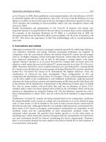
Based a description of shape memory alloy materials, a SMA Simulink block was developed.
The characteristic of material is idealized, but the approximations made are suitable for an
efficient simulation. The user can indicate the start and stop martensitic and austenitic
temperature and the force, momentum evolution.


Fig. 9. Configurable Simulink block for SMA material

The numerical results respect the real comportment of the user specified shape memory
alloy:

Biomimeticapproachtodesignandcontrolmechatronicsstructureusingsmartmaterials 339

 The Landau-Devonshire theory

 The mathematical model of Graesser and Cozzarelli
 The model of Stalmans, Van Humbeeck and Delaey
The Landau-Devonshire (Devonshire,1940) theory is one of the early models introduced.
The free energy  of SMA is a function of temperature T and strain  with positive constants
a
i
:

   
 

         
2 4 6
0 1 2 1 4 6
T, a a Tlog T a T T a a

(1)

The
 
 T, stress reaction of the material system, with

- material density, in varying the
order parameter, is proportional to the partial derivative of equation with respect to :

 


 
 



           



3 5
2 1 4 6
T,
T, 2a T T 4a 6a

(2)

Unfortunately the Landau Devonshire theory can only reproduce the isothermal
constitutive behavior of SMA. Neither the constant-stress transformation nor the free or
constrained memory effect can be modeled.
The mathematical model of Graesser and Cozzarelli (Graesser & Cozarelli, 1994) uses for
one dimensionality case only two basic equations. First equation is related to the stress rate


and the second equation determinates so-called one dimensional back stress :




   
 
    



 
 




 

n 1
E
Y Y

(3)

 




      




c
T
E f erf a
E

(4)

Three model parameters are directly related to material (elasticity modulus E, the slope of
inelastic region , the threshold stress Y) while the others have to be determined empirically
( f
T
controls the type and size of the hysteresis, c is assumed zero, n depends on influence in
forming the stress strain hysteresis, a describes the transition from the linear-elastic to the
inelastic region and the other way around).
The numerical stability of the model is the main advantage, but the model does not
consider the difference between martensite and austenite elasticity modulus.
The model of Stalmans (Stalmans,1994), Van Humbeeck and Delaey (Delaey,1987)0 was
developed to describe the change of one-dimensional composite material with embedded
SMA wires. Differentiation of the global equilibrium condition gives a generalized Clausius-
Clapeyron equation:
 

 
  
 
  
 
 
 
SMA 0
A
tr A V
, const
d s
C
dT

(5)

The material constant s is the entropy change during transformation from austenite to
martensite,

0
is the mass density of SMA material in stress free condition and



 
tr A V


is the transformation strain in dependence of the martensite volume fraction, C
A
represent
the gradient.
During transformation from martensite to austenite, the stress-rate is calculated during the
following equation:

 


 


  
    

  




spr matr
sma sma 0
mar sma
tr A V sma sma matr matr spr
SMA
mar
sma matr matr spr
k l
P E s
P E Q E k l
d
1 Q
dT
P Q E k l

(6)

The parameters implied in the last equation are:
l – the SMA matrix beam, P - the initial pseudo plastic strain, the cross section of the SMA
wire,
Q - pseudo elastic modulus,

- the average values of the thermal dilatation
coefficient,
E - the elasticity modulus. The subscript matr represent the specific parameters of

matrix beam to specific load or temperature.
The stress of the matrix material and the strain temperature can also be found out. However
the model can so far only describe the transformation from martensite to austenite.
Comparing the different models (Schroeder & Boller,1998) shows that each model has its
own characteristic. Each of the models still lacks the one or the other of the proprieties being
mentioned. A combination of models, such as done with the models of Stalmans and
Brinson leading to a new model called Stalman modified can result in an improvement of
the model’s proprieties.

3.5 Numerical tools for modelling shape memory alloy behavior
Based a description of shape memory alloy materials, a SMA Simulink block was developed.
The characteristic of material is idealized, but the approximations made are suitable for an
efficient simulation. The user can indicate the start and stop martensitic and austenitic
temperature and the force, momentum evolution.


Fig. 9. Configurable Simulink block for SMA material

The numerical results respect the real comportment of the user specified shape memory
alloy:

CONTEMPORARYROBOTICS-ChallengesandSolutions340


Fig. 10. The numerical simulation for Nitinol


Fig. 11. The response of SMA numerical model for sinusoidal thermal input
The electrical activation of SMA actuator imposes the following relations for the current,
temperature and response time:

For heating
   
2 2
I I I I
T 4,928 1,632 K K
Max T1 T2
2
d F
F
d
L
L

(7)

T
Max
- maximum temperature, d – wire diameter, I – electrical current, F
L
- required force




T T
Max
medium
t J ln
Heating
h

T T
Max

(8)

t
Heating
– heating time, Jh – heating coefficient, Tmedium – medium temperature, TA –
ambient temperature, T - aim temperature upon heating

   
1 2
2
h J J L
J 6,72 3,922d K K F

(9)

For cooling

 
 
H A
c c
c A S A
T T 28,88
t J ln
T T M T

(10)

   
c1 c2
2
c J J L
J 4,88 6,116d K K F

(11)

tc – cooling time, T
H
- initial temperature upon cooling, T
A
- ambient temperature, d –wire
diameter, T
C
- aim cooling temperature, J
C
- time constant for cooling, M - martensitic start
temperature.
One can observe the time dependence of required force and required stroke.
The electrical calculations for direct current heating determine:
 The amount of current needed for actuation in the required time
 The resistance of the nickel titanium actuation element
 The voltage required to drive the current through element
 The power dissipated by the actuation element.
The first requirement can be establish using the material description tables (Waram, 1993).
The resistance is determined using the following expression:



 
3
3
1,019x10
Resistance/mm /mm
d

(12)

The voltage and power requirements results from:


V IR ; 
2
Power I R

(13)
I – current in amps, V voltage in volts, R resistance in .
In case of using pulse width modulation heating the following relation can be used:

 

1
2
t
dut
y
c
y
cle % x100

t

(14)

t
1
– the width of constant current pulse, t
2
the total cycle time.

 

avr
i
100 P
duty cycle %
I R

(15)

 

avr
i
100
dut
y
c
y
cle % P R

V

(16)

P
avg
– average pulsed power (effective DC power), I
i
applied pulse current, V
i
applied
pulsed voltage, R electric resistance.

Biomimeticapproachtodesignandcontrolmechatronicsstructureusingsmartmaterials 341


Fig. 10. The numerical simulation for Nitinol


Fig. 11. The response of SMA numerical model for sinusoidal thermal input
The electrical activation of SMA actuator imposes the following relations for the current,
temperature and response time:
For heating
   
2 2
I I I I
T 4,928 1,632 K K
Max T1 T2
2
d F

F
d
L
L

(7)

T
Max
- maximum temperature, d – wire diameter, I – electrical current, F
L
- required force




T T
Max
medium
t J ln
Heating
h
T T
Max

(8)

t
Heating
– heating time, Jh – heating coefficient, Tmedium – medium temperature, TA –

ambient temperature, T - aim temperature upon heating

   
1 2
2
h J J L
J 6,72 3,922d K K F

(9)

For cooling

 
 
H A
c c
c A S A
T T 28,88
t J ln
T T M T

(10)

   
c1 c2
2
c J J L
J 4,88 6,116d K K F

(11)

tc – cooling time, T
H
- initial temperature upon cooling, T
A
- ambient temperature, d –wire
diameter, T
C
- aim cooling temperature, J
C
- time constant for cooling, M - martensitic start
temperature.
One can observe the time dependence of required force and required stroke.
The electrical calculations for direct current heating determine:
 The amount of current needed for actuation in the required time
 The resistance of the nickel titanium actuation element
 The voltage required to drive the current through element
 The power dissipated by the actuation element.
The first requirement can be establish using the material description tables (Waram, 1993).
The resistance is determined using the following expression:


 
3
3
1,019x10
Resistance/mm /mm
d

(12)

The voltage and power requirements results from:

V IR
; 
2
Power I R

(13)
I – current in amps, V voltage in volts, R resistance in .
In case of using pulse width modulation heating the following relation can be used:

 

1
2
t
dut
y
c
y
cle % x100
t

(14)

t
1
– the width of constant current pulse, t
2

the total cycle time.

 

avr
i
100 P
duty cycle %
I R

(15)

 

avr
i
100
dut
y
c
y
cle % P R
V

(16)

P
avg
– average pulsed power (effective DC power), I
i

applied pulse current, V
i
applied
pulsed voltage, R electric resistance.

CONTEMPORARYROBOTICS-ChallengesandSolutions342

4. Biomimetics design of mechatronics structure

4.1 Modular adaptive implant
Bionics or Biomechatronics is a fusion science which implies medicine, mechanics,
electronics, control and computers. The results of this science are implants and prosthesis
for human and animals. The roll of the implants and prosthesis is to interact with muscle,
skeleton, and nervous systems to assist or enhance motor control lost by trauma, disease, or
defect. Prostheses/implants are typically used to replace parts lost by injury (traumatic) or
missing from birth (congenital) or to supplement defective body parts. In addition to the
standard artificial limb for every-day use, many amputees have special limbs and devices to
aid in the participation of sports and recreational activities.

4.1.1 The parametric 3D model of the bones
To obtain the bone cross sections of the bones, a PHILIPS AURA CT tomograph installed in
the Emergency Hospital from Craiova was used –Fig. 12.


Fig. 12.
The PHILIPS AURA CT tomography

To obtain the tomography of the two bones (tibia and femur) were used two scanning
schemes presented in Fig. 13 ,Fig. 14 . For the ends of the bones the scanning operation was
made at the distances of 1 mm and for the medial areas at the distances of 3 mm.

Fig. 13.
Scanning schemes applied to the
femur
Fig. 14. Scanning schemes applied to the tibia

Were obtained 16 images folders and, after a strict selection, were used only 6, 3 for each
bone component including the upper and lower areas (scanned at 1 mm) and the medial
areas (scanned at 3 mm).
In Fig. 15 were presented two important images of the upper femur in the area of the
femoral head.


Fig. 15. Images obtained in the upper area of the femur

In Fig. 16 and Fig. 17 are presented main images of the medial and lower femur, which
shown the changes of the shape of the bone.

Biomimeticapproachtodesignandcontrolmechatronicsstructureusingsmartmaterials 343

4. Biomimetics design of mechatronics structure

4.1 Modular adaptive implant
Bionics or Biomechatronics is a fusion science which implies medicine, mechanics,
electronics, control and computers. The results of this science are implants and prosthesis
for human and animals. The roll of the implants and prosthesis is to interact with muscle,
skeleton, and nervous systems to assist or enhance motor control lost by trauma, disease, or

defect. Prostheses/implants are typically used to replace parts lost by injury (traumatic) or
missing from birth (congenital) or to supplement defective body parts. In addition to the
standard artificial limb for every-day use, many amputees have special limbs and devices to
aid in the participation of sports and recreational activities.

4.1.1 The parametric 3D model of the bones
To obtain the bone cross sections of the bones, a PHILIPS AURA CT tomograph installed in
the Emergency Hospital from Craiova was used –Fig. 12.


Fig. 12.
The PHILIPS AURA CT tomography

To obtain the tomography of the two bones (tibia and femur) were used two scanning
schemes presented in Fig. 13 ,Fig. 14 . For the ends of the bones the scanning operation was
made at the distances of 1 mm and for the medial areas at the distances of 3 mm.




Fig. 13.
Scanning schemes applied to the
femur
Fig. 14. Scanning schemes applied to the tibia

Were obtained 16 images folders and, after a strict selection, were used only 6, 3 for each
bone component including the upper and lower areas (scanned at 1 mm) and the medial
areas (scanned at 3 mm).
In Fig. 15 were presented two important images of the upper femur in the area of the
femoral head.

Fig. 15. Images obtained in the upper area of the femur

In Fig. 16 and Fig. 17 are presented main images of the medial and lower femur, which
shown the changes of the shape of the bone.

CONTEMPORARYROBOTICS-ChallengesandSolutions344


Fig. 16. Images obtained in the medial area of the femur


Fig. 17. Two images obtained in the lower area of the femur

In Fig. 18 , Fig. 19 and Fig. 20 important images of the upper tibia, the medial tibia and the
lower tibia, which show the shape changes of the bone, are presented.


Fig. 18. Four main images of the upper tibia


Fig. 19. Four main images made in the medial tibia area


Fig. 20. Four main images scanned in the lower tibia area

The obtained images were re-drawn in AutoCad over the real tomographies and the
drawings were imported in SolidWorks (a parametrical CAD software), section by section,
in parallel planes. The sketches made in the upper and lower areas for the femur bone and

for the tibia bone are presented Fig. 21, Fig. 22 and Fig. 23, Fig. 24.



Fig. 21. Sections for the femur bone – upper
femur
Fig. 22. Sections for the femur bone – lower
femur
Biomimeticapproachtodesignandcontrolmechatronicsstructureusingsmartmaterials 345


Fig. 16. Images obtained in the medial area of the femur


Fig. 17. Two images obtained in the lower area of the femur

In Fig. 18 , Fig. 19 and Fig. 20 important images of the upper tibia, the medial tibia and the
lower tibia, which show the shape changes of the bone, are presented.


Fig. 18. Four main images of the upper tibia


Fig. 19. Four main images made in the medial tibia area


Fig. 20. Four main images scanned in the lower tibia area

The obtained images were re-drawn in AutoCad over the real tomographies and the
drawings were imported in SolidWorks (a parametrical CAD software), section by section,

in parallel planes. The sketches made in the upper and lower areas for the femur bone and
for the tibia bone are presented Fig. 21, Fig. 22 and Fig. 23, Fig. 24.



Fig. 21. Sections for the femur bone – upper
femur
Fig. 22. Sections for the femur bone – lower
femur