Encyclopedia of Smart Materials (Vols 1 and 2) - M. Schwartz (2002) WW Part 5 ppt

P1: FCH/FYX P2: FCH/FYX QC: FCH/UKS T1: FCH
PB091-C2-Drv January 12, 2002 1:0
256 COMPOSITES, SURVEY
(a)
(d)
(b)
(c)
Figure 14. Schematic of the evolution of tensile fiber damage in
aligned fiber composites: (a) fiber break with interfacial debond-
ing, (b) fiber break expanding matrix crack, (c) matrix crack with
fiber bridging, and (d) a compilation of a, b, and c resulting in a
damage zone.
0
0.25
Fracture stress, σ →
G(σ) →
0.5
0.75
1.0
1
2
σ
l
σ
f
σ
u
Figure 15. Weibull cumulative probability distribution function
G(σ ) describing variations in fiber strength: (1) Fibers do not ex-
hibit a wide variability in fracture strength between 0 and 1, where

0.5 is the occurrence of tensile failure in 50% of fibers, and (2) a
wide variation exists and is statistically described by a standard
deviation as indicated with vertical lines.
σ
u
and the lower strength limit σ
l
, ω is a function of the
test sample aspect ratio and m depends on the amount of
scatter. The exponent m is approximately 1.2
σ/s, where
σ/s is the inverse of the coefficient of variation given by
σ
s
=


N
i=1
σ
i
N





N
i=1
(σ

i
− σ )
2
N

1/2


.
Below the lower strength limit, all fibers undergo the
same amount of elongation and remain unbroken. As the
lower strength limit is exceeded, the weakest fibers (those
containing internal flaws leading to reduced effective cross
sections) break in succession, and the load must be trans-
ferred to the surviving fibers. Complete fracture of the bun-
dle occurs when the upper strength limit is reached.
Several tensile dominated failure modes adopted to con-
sider the fiber-and-fiber bundle failure processes when
they are bound by a matrix include the weakest link fail-
ure mode, cumulative weakening failure mode, fiber break
propagation failure mode, and cumulative group failure
mode. The weakest link failure mode associates catas-
trophic failure with the occurrence of a single or isolated
small number of independent fiber breaks. Realistically,
this mode of failure is an unlikely characterization because
the stress level at which weakest link events occur would
not be sufficient enough to invoke composite material
failure.
The cumulative weakening failure mode is necessarily
an extension of the weakest link failure mode. Within char-

acterization of this mode, a fiber fracture site inhibits re-
distribution of stress near the site. As more sites develop
along a fiber, they tend to have a statistical strength distri-
bution that is equivalent to the distribution of flaws along
the fiber. Failure is thought to occur when a layer across
the section of a lamina is weakened to the point of not being
able to support any further increments in load. A critical
argument to acceptance of this mode entirely as a charac-
terization of failure is that no consideration is given to the
effects on neighboring fibers and flaws.
It is well known that the effects of stress perturbations
at terminations are significant to neighboring fibers. The
fiber break propagation failure mode is more realistic in
the sense that the effects of perturbations on the progres-
sive weakening of adjacent fibers are considered. As redis-
tribution of stress occurs, the stresses on adjacent fibers
are magnified, increasing the probability that failure will
occur in these fibers. With increased loading, the failure
probability increases until sequential fiber failure occurs.
Under auspices of the fiber break propagation model,
it is difficult to achieve a meaningful strength estimate,
and lamina tensile strength predictions generally depend
on the micromechanisms of deformation and fracture at
fiber termination points. For the smaller damaged vol-
umes of material, strength predictions are acceptable, but
predicted failure stresses are lower for larger volumes.
The cumulative group mode failure model considers the
effects of variability in fiber strengths, stress concentra-
tions in adjacent fibers arising from stress redistributions,
and the interfacial debonding process due to increased

matrix shear stresses. It is more likely that fiber breaks
P1: FCH/FYX P2: FCH/FYX QC: FCH/UKS T1: FCH
PB091-C2-Drv January 12, 2002 1:0
COMPOSITES, SURVEY 257
will progressively accumulate in groups between the stress
level necessary to initiate the first fiber break to the stress
level necessary to cause composite material failure. Com-
posite failure will occur when the distributed groups of
damage zones are of a sufficient number and size that
their cumulative effect reduces the material stiffness by
an amount sufficient enough to prohibit any additional
load-carrying capability. Weakening mechanisms by this
mode could be thought of in a couple of different manners.
In one way, the number of developed damage zones would
grow to such a number that the summed interactions ex-
ceeded the critical material stress. In another, the size and
number of zones would reach such magnitude that catas-
trophic and rapid crack propagation ensue due to the lack
of both intact material and crack tip blunting mechanisms
between zones. Although the cumulative group model sug-
gests a generalization of the cumulative weakening model,
the practicality of use is complicated by its complexity in
considering mostly all of the singular fiber longitudinal
tensile failure mechanisms.
The longitudinal compressive strength, like the longitu-
dinal tensile strength, is highly dependent on many factors
and is particularly sensitive to constituent matrix prop-
erties and fiber volume fraction. Several failure mecha-
nisms have been proposed, but the most dominant mecha-
nism is microbuckling, analogous to the buckling of a beam

on an elastic foundation. The surrounding matrix resists
fiber microbuckling, but there are several factors that can
lead to a reduction in the support given by the matrix and
neighboring fibers. At a low fiber volume fraction, the out-
of-phase or extensional buckling mode is suggested with
the lamina compressive strength predicted by the follow-
ing equation:
σ
cr
11,c
= 2V
f

V
f
E
m
E
f
3(1 − V
f
)
.
At higher, more industrially practicable fiber volume frac-
tions, the in-phase or shear bucking mode is suggested with
the lamina compressive strength predicted by the following
equation:
σ
cr
11,c

=
G
m
(1 − V
f
)
.
Given a constant fiber volume fraction, any factors con-
tributing to reduction in the matrix shear modulus will
lead to a reduction in composite compressive strength,
since the mode is in-phase. More specifically, the identified
factors that influence reduced support from the surround-
ing media include: (25)
r
Fiber bunching and waviness, which leads to prefer-
ential buckling, local matrix rich regions and matrix
instability.
r
The presence of voids, which tend to have a greater
effect than the matrix rich regions.
r
Interfacial debonding, due to circumferential tensile
stresses that arise principally from a difference in
Poisson’s ratios between the fibers and surrounding
matrix or the opposite effect induced by thermal cur-
ing stresses.
(b)
(a)
(c)
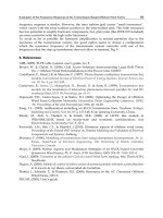
Figure 16. Progression of compressive fiber failure resulting

from longitudinal compressive in-phase buckling (a). In polymeric
aramid fibers, compressive yielding is common (b) during forma-
tion of a kink zone, while more pronounced kinking often leads to
fiber fracture at two locations (c) after (25).
r
A lower effective matrix shear modulus, compared to
the instantaneous matrix shear modulus, as a result
of viscoelastic deformation processes.
Another longitudinal compressive failure mechanism
specific to the structurally oriented, wholly aromatic
polyamide polymer fiber (Kevlar aramid) and carbon/
graphite fiber families, is the formation of kink-bands as
illustrated in Fig. 16. The highly anisotropic behavior of
these fibers lends to massive fiber rotation at one zone
and counter-rotation at another zone. In the extreme case,
compressive failure at the kink zones results in complete
fiber fracture at two locations. Compressive yielding with-
out complete failure is more typical of the polymeric Kevlar
aramids such as Kevlar 49.
The transverse tensile, compressive, shear, and longi-
tudinal shear strengths can be regarded as matrix domi-
nated, so the failure modes can be thought of as matrix-
modes of failure. Transverse tensile strength is governed
by the same factors as longitudinal compression, but with
one added detail. Unlike longitudinal tension where com-
posite strength is prescribed primarily on the basis of fiber
strength, the presence offibers in transverse tension havea
negative effect. Transverse strength is often lower than the
strength of the constituent neat matrix material because of
the stress magnification effects from fibers. Without regard

to the presence of stress magnification from fiber ends and
P1: FCH/FYX P2: FCH/FYX QC: FCH/UKS T1: FCH
PB091-C2-Drv January 12, 2002 1:0
258 COMPOSITES, SURVEY
matrix voids, the transverse strength is dictated primar-
ily by the interfacial bond strength. The interface is made
weaker when cohesive failure occurs prior to the cohesive
failure in either the constituent matrix or fibers.
Where interface bonding is weak, stress magnification
from fiber ends and voids tends to promote transverse
cracking more readily along the common edges of adjacent
fiber ends. These same factors also affect the transverse
and longitudinal shear strengths, depending on the direc-
tion of shear displacements and the viscoelastic properties
of the matrix. The only real differences here may be the
direction of crack propagation and the failure mode(s) of
the matrix, unless the fiber volume fraction is sufficiently
higher. If a large number of fibers are present and the inter-
facial bonding is good, the fibers will offer reinforcement,
provided the shearing plane is normal to the fibers. If the
shearing plane contains the fibers, then little fiber rein-
forcement is available and the strength is determined by
the properties of the matrix.
Identification of a predominant failure mechanism,
whether a fiber or matrix mode, is important from the per-
spective of designing composite structures. Knowledge of
the different failure mechanisms and the nature of single-
stress component damage initiation can be used to evalu-
ate the predominant mode of failure through formulation
of practical failure criteria. In establishing the failure cri-

terion, a fundamental assumption is that a failure criterion
exists to characterize failure in a UD composite and is of
the following form:
F(σ
11
,σ
22
,τ
12
) = 1,
where some function F is defined in terms of the princi-
pal stresses. A suitable failure criterion generally takes
the form of a quadratic polynomial because this is the sim-
plest form that has been found to adequately describe ex-
perimental data. The advantages are that several failure
criteria can be defined in terms of uniaxial strengths, and
a predominant mode of failure can be identified from the
criterion that is initially satisfied.
If a certain mode of failure is identified and deemed un-
desirable for a given load, the designer can tailor the com-
posite properties and re-evaluate the failure criteria until
some other mode is predicted that is less detrimental to the
design. For UD fiber composites, the general quadratic fail-
ure criterion is a two-dimensional version of the Tsai-Wu
criterion given by

1
S
t
1

S
c
1

σ
2
11
+

1
S
t
1
−
1
S
c
1

σ
11
+

1
S
t
2
S
c
2


σ
2
22
+

1
S
t
2
−
1
S
c
2

σ
22
−
1
2

1
S
t
1
S
c
1


1
S
t
2
S
c
2

1/2
σ
11
σ
22
+

1

S
s
12

2

τ
2
12
= 1,
where the S
ij
denote the single-component strengths and

the superscripts t, c, and s denote tension, compression,
and shear, respectively. The biggest drawback of this crite-
rion is that it ignores the diversity in the possible failure
modes.
Each of the failure modes previously mentioned can be
modeled as a specific criterion and, as such, evaluated and
identified independently. The following set of equations
provides a reasonable set of criteria for each of the domi-
nant fiber and matrix failure modes (26):
r
Tensile Fiber Failure

σ
11
S
t
1

2
+

τ
12
S
s
12

2
= 1.
r

Compressive Fiber Failure

σ
11
S
c
1

2
+

τ
12
S
s
12

2
= 1.
r
Tensile Matrix Failure

σ
22
S
c
2

2
+


τ
12
S
s
12

2
= 1.
r
Compressive Matrix Failure

σ
22
2S
s
23

2
+


S
c
2
2S
s
23

2

− 1


σ
22
S
c
2

+

τ
12
S
s
12

2
= 1.
Since the transverse shear strength S
23
is difficult to ob-
tain without performing thickness shear tests, the matrix
shear strength is used as an approximation. Upon evaluat-
ing each of the failure criteria for a given circumstance, the
predominant mode or modes of failure can be determined.
Necessarily, no biaxial tests are required, and a mode of
failure is identified by the criterion that is satisfied first.
MACROSCALE BEHAVIOR
On the macroscale, the effective composite elastic proper-

ties are evaluated on the basis of a composite laminate that
is composed of several laminae bonded together at various
orientations to one another. It was previously stated that
the composite structure or component and the laminate
may, in some cases, coincide on the same structural scale.
This being the case, tailoring laminate properties will also
coincide directly with influencing component behavior.
One of the most important aspects relating to the effec-
tive design of composite laminates and structures is knowl-
edge of composite lamina off-axis behavior and associated
limitations with particular fiber orientations. Aligned fiber
composite laminae are highly anisotropic in-plane, and
commonly varying degrees of coupling between extension
and shear occur when the direction of loading is not coinci-
dent with a principal material direction. The designer must
have some knowledge a priori of the lamina response to
off-axis loading conditions in order to determine a suitable
lamina lay-up sequence that provides optimum reinforce-
ment. An accurate prediction of laminate elastic proper-
ties, which are highly dependent on the orientation, prop-
erties, and distribution of individual laminae, is essential
for understanding the response of the resulting structure
to external loading and environmental conditions.
P1: FCH/FYX P2: FCH/FYX QC: FCH/UKS T1: FCH
PB091-C2-Drv January 12, 2002 1:0
COMPOSITES, SURVEY 259
Elastic Behavior Off-Axis
Hooke’s law can be generalized using a contracted form of
tensor notation and expressed concisely by the following
equation:

σ
i
=
6

j=1
C
ij
ε
j
,
where i, j = 1, ,6,σ
i
are the components of stress, C
ij
is
the stiffness matrix, and ε
j
are the components of strain.
Since the stiffness constants are symmetrical (i.e., C
ij
=
C
ji
), the expanded form of the previous equation is given
in matrix notation by









σ
1
σ
2
σ
3
τ
23
τ
31
τ
12








=









C
11
C
12
C
13
C
14
C
15
C
16
C
22
C
23
C
24
C
25
C
26
c
33
C
34
C

35
C
36
C
44
C
45
C
46
(SYM) C
55
C
56
C
66

















ε
1
ε
2
ε
3
γ
23
γ
31
γ
12








.
The constitutive relations that link stress to strain in
terms of the stiffness matrix may also be inverted to re-
late strain to stress in terms of the compliance matrix. The
constitutive relations for a UD composite lamina, which
exhibits orthotropic symmetry and transverse isotropy in
the x
2
–x

3
material principal coordinate plane, can be sim-
plified if the dimension in the x
3
(thickness) direction is
considered to be sufficiently smaller than both of the in-
plane dimensions. This consideration reduces the problem
to two dimensions, either of the plane stress or plane strain
form. Clearly, the implication is that the nonzero stresses
are arbitrarily restricted to in-plane; hence the nonzero
quantities are not functions of x
3
(σ
3
= τ
23
= τ
31
= 0). For
this, the stress-strain relation for a UD lamina given in
terms of the matrix of mathematical moduli [Q
ij
] becomes


σ
1
σ
2
σ

6


=


Q
11
Q
12
0
Q
12
Q
22
0
00Q
66




ε
1
ε
2
ε
6



,
where Q
11
, Q
22
, Q
12
, and Q
66
are identified as the reduced
stiffnesses.
The equation above suggests that no coupling exists be-
tween tensile and shear strains; that is, orthotropic com-
posite materials exhibit no shearing strains when applied
loads act coincident to the principal material directions.
The Q
ij
components of the reduced stiffness matrix from
this equation are given in terms of the engineering con-
stants as
Q
11
= C
11
=
E
11
1 − ν
12
ν

21
,
Q
22
= C
22
=
E
22
1 − ν
12
ν
21
,
Q
66
=
1
2
(C
11
− C
12
) = G
12
,
Q
12
= C
12

=
ν
12
E
22
1 − ν
12
ν
21
=
ν
21
E
11
1 − ν
12
ν
21
.
X
1
(Fiber direction)
X
2
(Transverse direction)
Z, X
3
(Thickness direction)
Y
X

λ
Figure 17. Representation of a UD composite lamina with the
principal material direction (fibers) oriented at some arbitrary in-
plane angle λ to the Cartesian coordinate X-Y plane.
When the direction of applied load does not coincide
with a principal material direction, then coupling between
tensile and shear strains exists. Consider the sufficiently
thin, UD lamina with fibers oriented at an angle λ to the
principal coordinate axis shown in Fig. 17. From classical
theory of elasticity, the stress–strain relation becomes


σ
x
σ
y
τ
xy


=


Q
11
Q
12
Q
16
Q

12
Q
22
Q
26
Q
16
Q
26
Q
66




ε
x
ε
y
γ
xy


,
where the
Q
ij
components of the matrix are referred to as
the transformed reduced stiffness components. In terms of
the reduced stiffness matrix components and λ, the trans-

formed reduced stiffness components have the following
values:
Q
11
= Q
11
cos
4
λ + 2(Q
12
+ 2Q
66
) sin
2
λ cos
2
λ + Q
22
sin
4
λ,
Q
22
= Q
11
sin
4
λ + 2(Q
12
+ 2Q

66
) sin
2
λ cos
2
λ + Q
22
cos
4
λ,
Q
66
= (Q
11
+ Q
22
− 2Q
12
− 2Q
66
) sin
2
λ cos
2
λ
+ Q
66
(sin
4
λ + cos

4
λ),
Q
12
= (Q
11
+ Q
22
−4Q
66
) sin
2
λ cos
2
λ + Q
12
(sin
4
λ+cos
4
λ),
Q
16
= (Q
11
− Q
12
− 2Q
66
) sin λ cos

3
λ
+(Q
12
− Q
22
+ 2Q
66
) sin
3
λ cos λ,
Q
26
= (Q
11
− Q
12
− 2Q
66
) sin
3
λ cos λ
+(Q
12
− Q
22
+ 2Q
66
) sin λ cos
3

λ.
If the local elasticproperties of the UD composite lamina
are known with respect to the material coordinate system,
the engineering elastic constants can be determined for the
Cartesian coordinate system as follows:
E
x
=

1
E
1
cos
4
λ+

1
G
12
−
2ν
12
E
1

sin
2
λ cos
2
λ+

1
E
2
sin
4
λ

−1
,
E
y
=

1
E
1
sin
4
λ+

1
G
12
−
2ν
12
E
1

sin

2
λ cos
2
λ+
1
E
2
sin
4
λ

−1
,
P1: FCH/FYX P2: FCH/FYX QC: FCH/UKS T1: FCH
PB091-C2-Drv January 12, 2002 1:0
260 COMPOSITES, SURVEY
0
0 10203040
Fiber orientation (λ) - degress
50 60 70 80
20
18
16
14
12
10
8
6
4
2

90
X
1
(Fiber direction)
X
2
(Transverse
direction)
Z, X
3
(Thickness direction)
Y
X
λ
G
xy
G
12
E
xx
E
22
V
xy
V
12
Figure 18. Variations of the engineering elastic constants
E
x
, G

xy
, and ν
xy
with the fiber orientation angle λ for a UD carbon-
epoxy composite of the following elastic properties: E
11
= 139.4
GPa (20.2 Msi), E
22
= 7.7GPa(1.1 Msi), G
12
= 3.0GPa(0.44 Msi),
ν
12
, = 0.3, and V
f
= 0.6.
G
xy
=

2

2
E
1
+
2
E
2

+
4ν
12
E
1
−
1
G
12

sin
2
λ cos
2
λ
+
1
G
12
(sin
4
λ + cos
4
λ)

−1
,
V
xy
= E

x

ν
12
E
1
(sin
4
λ + cos
4
λ)
−

1
E
1
+
1
E
2
−
1
G
12

sin
2
λ cos
2
λ


.
The variations of E
x
, G
xy
, and ν
xy
that result from these
equations, with the fiber orientation angle λ relative to the
principal material direction, are shown in Fig. 18 for a UD
carbon-epoxy composite. It is possible in some cases that
the predicted value of E
x
may exceed the values of E
11
and
E
22
depending on the differences among between G
12
, E
11
,
and E
22
. By carefully examining Fig. 18, one could envis-
age how the engineering elastic constants of a composite
laminate might be modified according to the orientations of
stacked laminae, hence allow performance tailoring char-

acteristics with composites.
Classical Lamination Theory
The most established theory for analysis of laminates takes
the form of the Kirchhoff hypothesis for thin plates or clas-
sical, linear, thin plate theory. Following the adaptation of
this theory for analysis of composite laminates, commonly
referred to as classical lamination theory (CLT), the sub-
sequent four assumptions are made:
r
Upon application of a load to a plate with a through-
thickness, lineal element normal to the plane of the
plate, the element undergoes at most a translation
and rotation with respect to the initial coordinate sys-
tem, but remains normal to the plate.
r
The plate resists in-plane and lateral loads only by
in-plane action, bending and transverse shear stress,
and not by through-thickness, blocklike tension or
compression.
r
There is a neutral plane, on which extensional strains
may not be zero but bending strains are zero in all
directions.
r
The laminate midplane is analogous to the neutral
plane of the plate.
According to the foregoing assumptions for adaptation
of the Kirchhoff hypothesis for thin plates, the strain com-
ponents can be derived from the midplane strains and
curvatures. The midplane strains are expressed as ε

◦
xx
=
∂u
◦
/∂x,ε
◦
yy
= ∂v
◦
/∂y and γ
◦
xy
= (∂u
◦
/∂y) + (∂v
◦
/∂x), where
u
◦
and ν
◦
are expressed in terms of the x and y coordi-
nate directions. The midplane curvatures are expressed as
κ
xx
=−∂
2
w
◦

/∂x
2
, κ
yy
=−∂
2
w
◦
/∂y
2
, and κ
xy
=−∂
2
w
◦
/∂x∂ y
and are related to the z coordinate direction. Here κ
xy
refers
to the curvature of twist about the plane of the plate. The
strain components are expressed in matrix form as



ε
x
ε
y
γ

xy



=



ε
x,0
ε
y,0
γ
xy,0



+ z


















−
∂
2
w
∂x
2
−
∂
2
w
∂y
2
−2
∂
2
w
∂x∂ y


















,
{
ε
}
=
{
ε
}
0
+ z
{
κ
}
0
.
The equation above implies that the strains vary lin-
early with z, meaning that through-thickness sections re-
main plane and normal after deformation relative to the
original coordinate system with its origin at the midplane.
If the strains vary linearly, then lamina (ply) stresses must
vary in proportion to lamina stiffnesses. In terms of the

laminate, the ply stress components are given by
{
σ
}
κ
=

Q
xy

κ
{
ε
}
κ
=

Q
xy

κ
{
ε
}
0
+ z
κ

Q
xy


κ
{
κ
}
0
,
where the subscript k denotes the contribution from the
kth ply within the composite laminate. According to the
plate shown in Fig. 19, the forces and moments have a lin-
eal distribution. In reference to the stress components for
the kth ply in the previous equation, force and moment
equilibrium are considered. The forces and moments that
are responsible for producing in-plane ply stresses are de-
noted by N
x
, N
y
, N
xy
, M
x
, M
y
, and M
xy
, where the N ’s are
the ply-level forces and the M ’s are the ply-level moments.
For force equilibrium, the integrated, through-thickness
laminate stress must be equivalent to the corresponding

force that produces it. The total force and moment, deter-
mined from contributions of all plies within the laminate,
P1: FCH/FYX P2: FCH/FYX QC: FCH/UKS T1: FCH
PB091-C2-Drv January 12, 2002 1:0
COMPOSITES, SURVEY 261
M
y
Results in σ
y
M
x
Results in σ
x
M
xy
Results in τ
xy
N
y
N
xy
N
xy
N
x
Q
y
Q
x
Y

X
Z
Figure 19. In-plane force and the moment resultants of a lami-
nated plate subjected to extensional forces and bending moments.
can be expressed as



N
x
N
y
N
xy



=
n

k=1
h
k

h
k−1
(σ
x,k
,σ
y,k

,τ
xy,k
)dz ,
{N}=



n

k=1
[Q
xy
]
k
h
k

h
k−1
dz



{ε}
0
+



n


k=1
[Q
xy
]
k
h
k

h
k−1
zdz



{κ}
0
=

n

k=1
(h
k
− h
k−1
)[Q
xy
]
k


{ε}
0
+

n

k=1
1
2

h
2
k
− h
2
k−1

[Q
xy
]
k

{κ}
0
= [A]{ε}
0
+ [B]{κ}
0
,




M
x
M
y
M
xy



=
n

k=1
h
k

h
k−1
(σ
x,k
,σ
y,k
,τ
xy,k
)zdz ,
{M}=




n

k=1
[Q
xy
]
k
h
k

h
k−1
zdz



{ε}
0
+



n

k=1
[Q
xy
]

k
h
k

h
k−1
z
2
dz



{κ}
0
=

n

k=1
1
2

h
2
k
− h
2
k−1

[Q

xy
]
k

{ε}
0
+

n

k=1
1
3

h
3
k
− h
3
k−1

[Q
xy
]
k

{κ}
0
= [B]{ε}
0

+ [D]{κ}
0
.
The peculiar mechanical behavior of composite lami-
nates can be discerned by examining the two previous
equations. The first equation implies that changes in cur-
vature (bending strains), stretching and squeezing are
brought about by the tensile forces and compressive forces
given by {N}. Also the second equation implies that the mo-
ments given by {M}, in addition to changes in curvature,
can produce squeezing and stretching strains. From the
force and moment equilibrium analysis, the constitutive
relations for laminated composites can be expressed in a
condensed form as follows:

N
M

=

A
B
B D

ε
0
κ
0

,

where the A, B, and D matrices are the extension, exten-
sion-bending coupling and bending stiffnesses, respec-
tively. Upon expansion of the condensed form, the solution
to the stiffnesses can be written in terms of summations
of transformed, reduced stiffnesses belonging to individual
laminae having h
k
th thicknesses:
[
A
]
=
n

k=1
(h
k
− h
k−1
)[Q
xy
]
k
,
[
B
]
=
n


k=1
1
2

h
2
k
− h
2
k−1

[Q
xy
]
k
,
[
D
]
=
n

k=1
1
3

h
3
k
− h

3
k−1

[Q
xy
]
k
.
Evaluation of the extension, extension-bending coup-
ling and bending stiffnesses, or more simply, the [ABD]
matrix serves many purposes in the analysis of composite
laminates. This matrix has many uses from the standpoint
of designing composite laminates and engineering struc-
tures, and it may be used for the following (27):
r
Calculating the effective composite laminate elastic
properties.
r
Calculating the ply-level stresses and ply-level strains
for a given load on the laminate.
r
Calculating the ply-level stresses and laminate load
for a given mid-plane strain.
r
Evaluating whether bending strains would result
from an extensional load, and vice versa.
r
Comparative evaluations of different lay-ups followed
by optimization.
r

Determining the variation of laminate properties
along different directions.
r
Calculating the thermal expansion and swelling coef-
ficients of the laminate.
r
Estimating the laminate residual stresses due to
curing.
r
Calculating the ply-level hygral and thermal stresses.
Effects of Orientation and Stacking
The derivation of the [ABD] matrix suggests that the
elastic behavior of a composite laminate made from UD
laminae is influenced by the constituent fiber and matrix
properties as well as the orientations and locations of in-
dividual laminae with respect to the geometric midplane
of the laminate. The extensional [A] matrix relates the
stress resultants with the midplane strains, and the nor-
mal stress resultant-to-midplane shearstrain coupling and
shear stress resultant-to-midplane normal strain coupling
P1: FCH/FYX P2: FCH/FYX QC: FCH/UKS T1: FCH
PB091-C2-Drv January 12, 2002 1:0
262 COMPOSITES, SURVEY
are due to the A
16
and A
26
components, respectively. The
B
16

and B
26
components of the extension-bending coupling
[B] matrix relate the normal stress resultants with lami-
nate twisting, and the [B] matrix also suggests the coupling
between the moment resultants and the in-plane strains.
Finally, the interaction between the laminate bending mo-
ment and laminate twisting are related through the D
16
and D
26
terms of the bending [D] matrix (28). A physical
sense of the coupling effects that exist in relation to the
laminate midplane can be seen in Fig. 20(a–b).
If an isostrain condition is assumed for the laminae
shown in Fig. 20(a), different stresses will result normal
and transverse to the laminae due to their orthotropic be-
havior. Then, upon bonding and releasing of applied stress,
the laminate will distort and bend favorably toward the
lamina with higher in-plane stiffness. For the laminate to
remain flat, an additional force normal to the plane would
be necessary. Similarly, if a uniaxial stress were applied
to a laminate having laminae oriented at +/−λ and lack-
ing end constraints as shown in Fig. 20(b), twisting about
the axis would result due to the extensional-shear coupling
arising from anti-symmetry about the midplane.
From a practical standpoint, it is useful to minimize
or eliminate these coupling effects, since most engineer-
ing structures are required to maintain dimensional sta-
bility for long periods of time under various loading and

environmental conditions. According to the premises of the
[ABD] matrix, coupling can be minimized by selecting the
appropriate sequences in which to lay-up individual lam-
inae having various materials, thicknesses, and orienta-
tions. This may be referred to as the design of composite
laminates and engineering structures.
Two of the most important classes of composite lam-
inate designs from an engineering perspective are sym-
metric laminates and quasi-isotropic laminates. In sym-
metric laminates, laminae (plies) on opposing sides of the
laminate geometric midplane have the same material,
thickness, and orientation. Symmetry about the midplane
eliminates the undesirable effects of extension-bending
coupling; that is, all of the elements in the [B] matrix be-
come zero and unknown residual stresses from warping
deformation are avoided. Except for the cases of cross-ply,
all 0
◦
, or all 90
◦
, bending moments in symmetric laminates
still produce torsional deflections ([D] matrix). However,
the magnitudes can be reduced by increasing the number
of plies, for example, in cross-ply configurations.
The notation often adopted in describing a lay-up that
is symmetric is as follows: a six-layered stacking se-
quence expressed as [0
◦
/−45
◦

/+45
◦
2
/−45
◦
/0
◦
] is equiv-
alent to the sequence denoting symmetry expressed as
[0
◦
/−45
◦
/+45
◦
]
S
provided that the thicknesses and mate-
rials are matched below the midplane. The term “quasi-
isotropic” as used to describe laminate behavior suggests
the same [A] matrix in all directions. Quasi-isotropic lami-
nates exhibit very little variation in apparent elastic mod-
uli with direction, and this becomes useful when the load-
ing direction is unknown or variable.
From the perspective of designing laminates, a lami-
nate can be made isotropic, or nearly isotropic, by having a
number of plies greater than four that are equal in thick-
ness and oriented by 2π/n (n is the total number of plies) to
ε
1

ε
1
ε
2
ε
2
90°
0°
(a)
−λ
σ
σ
+λ
(b)
Figure 20. Interpretation of the coupling effects between two
bonded composite laminae at various orientations with respect
to the geometric midplane: (a) Extensional-bending coupling in
well-bonded laminae oriented at 0 and 90
◦
under isostrain condi-
tions, and (b) extensional-shear coupling, which produces twisting
in well-bonded laminae oriented at +λ and −λ to the principal ma-
terial axis.
adjacent plies. Ideally, quasi-isotropic laminates are sym-
metric, and symmetric or unsymmetric laminates are at
least balanced in thickness, since these designs will tend to
be most well-behaved structurally and at least somewhat
predictable in response. Examples of symmetric and un-
symmetric composite laminate lay-up sequences are shown
in Fig. 21.

P1: FCH/FYX P2: FCH/FYX QC: FCH/UKS T1: FCH
PB091-C2-Drv January 12, 2002 1:0
COMPOSITES, SURVEY 263
h
1
h
1
h
1
h
1
h
1
h
1
h
1
h
1
1.5 h
1
h
1
h
1
1.5 h
1
1.5 h
1
h

1
h
1
h
1
1.5 h
1
h
1
h
1
h
1
1.5 h
1
h
1
1.5 h
1
1.5 h
1
h
1
h
1
h
1
h
1
h

1
h
1
h
1
h
1
+λ
+λ
−λ
+λ
−λ
+λ
−λ
−λ
90°
90°
90°
90°
90°
0°
0°
0°
90°
90°
0°
0°
90°
0°
90°

0°
90°
90°
0°
0°
90°
90°
0°
0
Symmetric
Non-Symmetric
Figure 21. Examples of symmetric and nonsymmetric laminates for the general 0
◦
/90
◦
cross-ply
and +λ/ − λ angle-ply configurations.
Laminate Failure
Identification of the precise manner in which a compos-
ite may fail depends not only on the composite architec-
ture but also on the conditions to which it is exposed. For
the purposes of engineering design, it is somewhat less of
an arduous task to at least estimate when the composite
may fail rather than how it will fail. Failure of a compos-
ite may be restrictively considered when failure of the first
lamina occurs or more realistically considered when the
composite can no longer support any additional load. The
first situation is often referred to as the first-ply-failure
(FPF) philosophy, and the second situation is referred to as
the ultimate-laminate-failure (ULF) philosophy. With FPF,

the inverted [ABD] matrix is used to evaluate the midplane
strains and curvature changes in accordance with the ap-
plied load vector. Upon evaluating the strains, the stresses
in the principal material coordinate system can be calcu-
lated and used with any of the composite failure criteria
to determine if the applied load vector satisfies a failure
P1: FCH/FYX P2: FCH/FYX QC: FCH/UKS T1: FCH
PB091-C2-Drv January 12, 2002 1:0
264 COMPOSITES, SURVEY
condition. Knowledge of when the first ply failure occurs
can lead to appropriate choices for laminate safety factors
in design.
ULF extends the application of FPF to the entire lam-
inate. Rather than considering the composite as “failed”
once the FPF load is reached, the properties of the failed
ply are reduced to values incapable of sustaining load. The
“new” composite is re-evaluated, whereby the process is
repeated in an iterative fashion until the plies remaining
can no longer support any load. At this point, the compos-
ite is considered to have failed. Although less conservative
than the FPF approach, the ULF approach does offer merit
in the sense of capturing the progressive stiffness changes
that occur prior to ultimate failure. In this manner, the
ULF approach is similar to the classical techniques avail-
able for metals.
OTHER CONSIDERATIONS
The particular mechanical behavior associated with com-
posite laminates and structures involves the interactions
of many materials on distinct geometric scales. Principles
fundamental to the treatment of composite performance

in the elastic regime have been presented, notwithstand-
ing considerations for environmental conditions and that
new material technologies must also be ascertained. Many
applications that are emerging where composite materials
may be employed as suitable replacements involve long-
term durability in hot and wet conditions. Here knowledge
of the hygrothermal effects in a specific composite becomes
critical to the design process.
Stresses can be developed in individual plies when they
are constrained by neighboring plies against dimensional
changes due to thermal and hygroscopic expansions. The
distribution of stresses from hygrothermal effects are a
function of ply orientation, and the resulting deformation
due to these effects may be evaluated by considering the
total strain minus the mechanical strain. Since thermal
diffusion takes place in composites at a much faster rate
than moisture diffusion, the nonmechanical strains due to
thermal and moisture exposure may be treated as compo-
nent effects.
In addition to the continued development of techniques
for evaluating the behavior of composites exposed to var-
ious environmental conditions, further understanding of
the peculiarities with composites is also necessary for fu-
ture growth toward that of “smarter” structures. That is,
such composite structures would not only receive external
stimuli in a positive manner but also provide predictable
and measurable feedback to those stimuli. To capitalize
on the benefits from these structures, designers must ex-
plore many of the unresolved issues within the regimes of
understanding nonlinear behavior, new (hybrid) material

interactions, and constitutive material relations. For ex-
ample, if we want a material that exhibits piezoelectric,
electrostrictive, or magnetostrictive characteristics, then
we would introduce phases that exhibit these behaviors.
However, the presence of these phases could also result
in more complicated predictions of composite behavior due
to their interactions and resulting stress redistributions.
Since these phases might be incorporated to inhibit some
type of linear or nonlinear response to external stimuli in
the first place, the current framework of linear elastic the-
ory may not offer reasonable answers. Consequently, much
greater opportunity now exists to offer new theories and
ideas to the already established and rapidly progressing
comprehension of composite material behavior.
BIBLIOGRAPHY
1. M.F. Ashby. Materials Selection in Mechanical Design.
Pergamon Press, Oxford, 1992, pp. 1–15.
2. W.D. Compton and N.A. Gjostein. Sci. Am. 255: 92–100 (1986).
3. T.W. Chou. Microstructural Design of Fiber Composites.
Cambridge University Press, Cambridge, 1992, pp. 10–11.
4. R.A. Flinn and P.K. Trojan. Engineering Materials and Their
Applications, 4th ed. Houghton Mifflin, Boston, 1990, pp. 703–
709.
5. D. Hull, An Introduction to Composite Materials. Cambridge
University Press, Cambridge, 1981, pp. 1–5.
6. M.A. Meador, P.J. Cavano, and D.C. Malarik. Proc. 6th
Ann. ASM/ESD Advanced Composites Conference. Detroit,
Michigan, 1990, pp. 529–539.
7. R.D. Vannucci. Proc. 32nd Int. SAMPE Symp. Anaheim, CA,
April 6–9, 1987.

8. L.H. Sperling. Introduction to Physical Polymer Science, 2nd
ed. Wiley, New York, 1992, p. 527.
9. A.V. Pocius. Adhesion and Adhesives Technology: An Introduc-
tion. Hanser Munich, 1997, p. 81.
10. S.I. Krishnamachari. Applied Stress Analysis of Plastics: A
Mechanical Engineering Approach. Van Nostrand Reinhold,
New York, 1992, p. 355.
11. B.N. Cox and G. Flanagan. Handbook of Analytical Methods
for Textile Composites. NASA Contractor Report 4750 (1–33).
NASA Langley Research Center, Hampton, VA., March 1997,
pp. 2:1–2:4.
12. J.C. Halpin and S.W. Tsai. Environmental factors in composite
materials design. Air Force Materials Laboratory Technical
Report AFML-TR-67–423, 67–423 (1967).
13. C.C. Chamis. Proc. 38th Ann. Conf. Society of Plastics Industry
(SPI). Houston, TX, February, 1983.
14. Z. Hashin and B.W. Rosen. J. Appl. Mech. 31: 223–232 (1964).
15. Z. Hashin. J. Appl. Mech. 46: 543–550 (1979).
16. Z. Hashin. J. Appl. Mech. 50: 481–505 (1983).
17. T. Ishikawa and T.W. Chou. J. Mat. Sci. 17: 3211–3220 (1982).
18. T. Ishikawa, M. Matsushima, and Y. Hayashi. J. Comp. Mat.
19: 443–458 (1985).
19. N.K. Naik and P.S. Shembekar. J. Comp. Mat. 26: 2196–2225
(1992).
20. N.K. Naik, P.S. Shembekar, and M.V. Hosur. J. Comp. Tech.
Res. 13: 107–116 (1991).
21. T.J. Walsh and O.O. Ochoa. Mech. Comp. Mat. Struct. 3: 133–
52 (1996).
22. K.H. Searles. The Elastic and Failure Behaviors of 8HS
Woven Graphite Fabric Reinforced Polyimide Composites.

Ph.D. thesis. Oregon Graduate Institute of Science and Tech-
nology, 1999.
23. K. Searles, G. Odegard, and M. Kumosa. Mech. Comp. Mat.
Struct. 1999, in press.
24. T. Akasaka. Comp. Mat. Struct. Jpn 3: 21–22 (1974).
25. D. Hull. An Introduction to Composite Materials. Cambridge
University Press, Cambridge, 1981, pp. 156–157.
P1: FCH/FYX P2: FCH/FYX QC: FCH/UKS T1: FCH
PB091-C2-Drv January 12, 2002 1:0
COMPUTATIONAL TECHNIQUES FOR SMART MATERIALS 265
26. Z. Hashin. J. Appl. Mech. 47: 329 (1980).
27. S.I. Krishnamachari. Applied Stress Analysis of Plastics: A
Mechanical Engineering Approach. Van Nostrand Reinhold,
New York, 1992, p. 419.
28. T.W. Chou. Microstructural Design of Fiber Composites.
Cambridge University Press, Cambridge, 1992, pp. 44–45.
COMPUTATIONAL TECHNIQUES
FOR SMART MATERIALS
MANUEL
LASO
JUAN
L. CORMENZANA
ETSII / Polytechnic University of Madrid
Madrid, Spain
INTRODUCTION
In the following sections, we will use the term “design” in
a rather restricted sense. Specifically, we will refer to the
calculations, simulations, or in general to any quantita-
tive approach necessary to specify a structure, part, mech-
anism, processing operation, or function, in which a smart

material is used.
In a large number of cases, the design with smart
materials relies on well-known and established principles
of thermodynamics and continuum mechanics, such as the
theories of elasticity (1), fluid mechanics (2), classical elec-
tromagnetic field theory (3), chemical equilibrium and ki-
netics, and solid state physics (4). These theoretical frame-
works typically result in a consistent set of equations, of
which at least one relates the stimulus and the response
of the system. The design task consists often in specifying
dimensions of structures or operating conditions of devices
that guarantee satisfactory function. A typical example is
the design of a smart structure that, under changes in tem-
perature, deforms in a controlled way, possibly operating a
valve or tripping a relay switch. The design of such a com-
ponent, involves a straightforward application of the laws
of thermoelasticity, provided that the thermomechanical
properties of the material are known.
The controlling principles can often be expressed as very
concise and elegant partial differential equations (PDEs)
that must be satisfied in domains of complicated shape that
have rather involved boundary and initial conditions. This
combination of highly nonlinear PDEs, boundary, and ini-
tial conditions makes an analytical approach impossible in
most cases. Approximate numerical techniques like finite
differences (FD), finite elements (FE), finite volumes (FV),
spectral methods (SM) and the like are then resorted to of-
ten with spectacular success in mechanical and electrical
engineering and fluid mechanics (5–7).
In other cases, the difficult part of the design task is not

the structural, fluid-mechanical, optical or thermal design
itself, but the description of the behavior of the smart mate-
rial (8). The behavior of a material has been tradition-
ally represented by a so-called constitutive equation (CE)
that, put in very broad terms, links stimulus and response.
Constitutive equations are used daily in design tasks,
sometimes even without our realizing it. For example, one
of the simplest CEs is the linear relationship between the
tensorial magnitudes strain and stress for a linearly elastic
material, which in its more general form, that is, valid
also for anisotropic materials and using the convention of
summation over repeated indexes (1), has the following
aspect:
σ
ik
= λ
iklm
u
lm
. (1)
This expression basically makes the deformation of a ma-
terial proportional to the cause (stress) and includes, as a
special case, Hooke’slaw
u
zz
=
σ
zz
E
, (2)

where E is Young’s modulus.
This very simple CE can be said to be the basis of
the vast majority of isothermal linear elastic structural
designs. Similarly, most of computational fluid dynamics
(CFD) makes use of Newton’s relationship between stress
and a velocity gradient:
˜
τ =−η ˙
˜
γ, (3)
where ˙
˜
γ = (
¯
∇
¯
v) + (
¯
∇
¯
v)
T
is the strain rate and η is the vis-
cosity.
Again, this very simple CE has extremely wide appli-
cability, smart materials included. A key point worth em-
phasizing in this context is the fact that constitutive equa-
tions are postulates and therefore have a certain degree of
arbitrariness. They do not follow from general fundamen-
tal principles, as conservation laws do, although they have

to conform to certain deeply rooted requirements. Thus,
a design problem involves typically a set of fundamen-
tal laws, expressed in one of several possible and more or
less general ways (thermodynamic, chemical or mechanical
equilibrium, conservation of energy, mass and momentum,
minimization of action, and minimization of free energy)
together with one or more CEs that characterize the ma-
terial used. The fundamental conservation or variational
laws are universal and have to be obeyed by any material
we care to consider (Fig. 1).
By way of example, consider now the design of an
isothermal flow process of a smart material that behaves
as an incompressible memory or viscoelastic fluid. In this
case, the fundamental laws that must be satisfied so that
the design has physical sense are just two:
(
¯
∇·
¯
v) = 0 (conservation ofmass), (4)
ρ
∂
∂t
¯
v + [
¯
∇·ρ
¯
v
¯

v] + [
¯
∇·
˜
π] = 0(conservation of linear
momentum), (5)
where
˜
π is the total momentum-flux or total stress tensor
which can be split in the following way:
˜
π =−p
˜
δ +
˜
τ,
where p is the pressure and
˜
τ is the stress tensor due to
the fluid.
˜
τ is as yet unspecified. We need a CE to define
it and close the system of equations. The goodness of our
P1: FCH/FYX P2: FCH/FYX QC: FCH/UKS T1: FCH
PB091-C2-Drv January 12, 2002 1:0
266 COMPUTATIONAL TECHNIQUES FOR SMART MATERIALS
Conservation law,
equilibrium law,
minimization law, etc.
e.g. conservation

of linear momentum,
conservation
of energy
Constitutive
equations
e.g. Newtonian fluid,
Fourier's law for
thermal transport,
constant density, etc.
Integration domain,
boundary and initial
conditions
e.g. object shape,
temperature in
surroundings, etc.
Design
problem
solution
e.g. shape,
velocity and
temperature
fields, etc.
Figure 1. Basic structure of the design task. Conservation laws
form an incomplete set of equations that must be closed by one or
more constitutive equations.
design will depend critically on the precise form we give
to
˜
τ , that is, on the way the stress in the fluid is going to
depend on its velocity or on the history of the flow.

This CE, on the other hand, is entirely specific for our
material. For example, if the material seems to behave as
a Newtonian fluid during processing, the most reasonable
CE would be Eq. (3). But this is not, of course, our only
choice. Within certain boundaries, we are free to specify
any relationship between stimulus and response (between
strain rate and stress in this case). Even the roles of stimu-
lus and response are interchangeable under some circum-
stances.
It is often useful to think of the CE as a kind of
“calculator” that, when fed a value of the stimulus (say, a
strain rate), gives us back the response of the material (say,
a stress). This calculator typically contains one or more
free parameters that are obtained from a fit to experimen-
tal measurements and are specific for the material under
consideration. These free parameters are often referred to
as “material properties.” Typical material properties are
viscosity, elastic modulus, diffusion coefficient, thermal dif-
fusivity, and optical linear and nonlinear susceptibility. In
this discussion, it is assumed that material properties are
known. In many cases, this assumption entirely eliminates
the difficulty of the problem, which often is the characteri-
zation of the material. We are dealing here with design
problems in which the material is perfectly known, but its
behavior in a complex situation has to be determined.
The conservation, equilibrium, or minimization laws
form a consistent but incomplete set of equations that re-
quire so-called “closure” to become solvable. The CE is the
closure. CEs are so often taken for granted, that their very
special nature is easily forgotten. It suffices to think of the

Navier–Stokes equations, on which most CFD is based: the
Navier–Stokes equations are almost automatically taken
for granted as the foundation of fluid mechanics. But in fact
they are already a combination of the momentum conser-
vation equation and the CE for the Newtonian fluid: they
can be obtained by plugging Eq. (3) into Eq. (5) and as-
suming that the fluid has constant density. Consequently,
whenever we use them to design a flow system, we are au-
tomatically and tacitly assuming that the flowing mate-
rial obeys a very special and simple Newtonian CE.
Furthermore, looking beyond the fact that different New-
tonian fluids have different numerical values of viscosity,
there is only one Newtonian fluid. The same is true for
a perfectly elastic solid. All Newtonian fluids, all linear
elastic solids, all linear optical materials behave in essen-
tially one and the same way. Therefore, as soon as it is
postulated that a smart material obeys one of these sim-
ple CEs, the design task becomes relatively simple. It will
require only the same standard techniques used for non-
smart materials. Such techniques may, of course, be very
involved themselves (think of turbulent CFD), but they do
not differ fundamentally from the techniques used to de-
sign for less smart materials. We will informally call such
“standard” cases “design problems of the first kind.” They
probably constitute 75% of all design tasks in which smart
materials are involved. Because the techniques used for
problems of the first kind are the same as those for non-
smart materials, they will not be dealt with here in any
depth.
In the remaining 25% of the design problems for smart

materials, the sophisticated numerical machinery deve-
loped during the last four decades is not sufficient to pro-
vide reliable solutions in a reasonable time. We will call
these “design problems of the second kind.”
The coming sections will be devoted to the two main as-
pects in which the design and calculation for smart materi-
als departs significantly from standard design techniques.
Both aspects are intimately related to the CE or, somewhat
ironically, to its nonexistence. We have already seen that
the conservation equations are the same for smart and less
smart materials. It is the additional complication brought
about by the CE that distinguishes these special design or
calculation problems.
The first aspect specific of CEs for smart materials has
to do with the existence of memory effects. As a matter of
fact, some of the most spectacular effects that smart ma-
terials display are related to what is somewhat vaguely
called memory. The next section discusses some general
aspects of memory in materials and its mathematical for-
mulation. In the following section, we consider the question
how to handle materials that have memory in practical cal-
culations. Finally, the subsequent section deals with the
more fundamental question how to postulate a constitu-
tive equation for smart materials. These last two sections
reflect some recent developments in fields that are rapidly
developing. A tentative outlook into the future of designing
smart materials is presented in the closing section.
SMART MATERIALS, MEMORY EFFECTS,
AND MOLECULAR COMPLEXITY
Frequently, complicated material behavior is closely

related to the concept of memory, a key word very often
heard in the context of smart materials. For example,
form or shape memory materials constitute one of the
best known classes of smart materials mainly due to the
spectacularity of some of its applications (9). Less widely
known, but also capable of displaying a stunning range of
P1: FCH/FYX P2: FCH/FYX QC: FCH/UKS T1: FCH
PB091-C2-Drv January 12, 2002 1:0
COMPUTATIONAL TECHNIQUES FOR SMART MATERIALS 267
nontrivial and often counterintuitive behavior, the large fa-
mily of complex fluids has found numerous applications
as smart materials. Smart materials based on complex
fluids include gels, polymeric melts and solutions, colloidal
dispersions, electro- and magnetorheological fluids, and
liquid crystalline materials among others (10–13). All
of these materials share some or all of the following
characteristics, which are in many cases responsible for
their smart behavior:
r
They possess the ability to react to external excita-
tions (fields, pH changes, strain) in a highly nonlinear
way and often undergo a phase change.
r
They display their most interesting behavior when
driven strongly away from equilibrium.
r
They typically possess either a very wide spectrum of
relaxation times or else a main relaxation time, whose
order of magnitude is comparable with the timescale
of the physical process in which they find application

(14).
r
They often have a complicated small-scale structure,
either at the molecular level (polymers) or at some
mesoscopic scale (dispersions, emulsions, polycrys-
talline materials).
Although there is no single mechanism responsible for
memory, several of these characteristics are responsible for
phenomena such as hysteresis and memory. In some cases,
a material appears to have a fading memory of past events
because its internal structure (e.g., molecular) requires a
certain time to adapt to a changing environment. Thus,
memory is also a question of the timescale in which the
relevant material property is observed. We can take water
as an example. It is a low molecular weight fluid that be-
haves as a simple Newtonian fluid in most cases because
its characteristic molecular relaxation time is very short
compared with the characteristic times of flow in everyday
life. Thus, it can adapt instantly to changes in the velo-
city field and therefore displays no memory effect. On the
other hand, a high molecular weight polymer has a spec-
trum of relaxation times that can reach well into seconds.
Any stimulus, for example, a change in an electric field,
that tries to change its orientation will be followed by an
observably slow response, during which the material re-
tains information about the past state.
In other cases, memory is due to a kinetically frozen-in
state, for example, due to a martensitic–austenitic phase
transition, which can be unlocked by applying an external
stimulus. The material is then forced to revert to a previous

state and thus appears to possess memory.
There have been several attempts to capture these phe-
nomena in a mathematical formulation. At this point, in-
stead of addressing the question in an all-encompassing
and general way, we will rather continue with our specific
example, which is a representative example of materials
that have complex behavior. We will address the family of
high molecular weight polymers, which are considered by
many as memory fluids par excellence.
Polymers display strong memory effects that are a
consequence of their non-Newtonian nature and ulti-
mately of their complex molecular structure and of the
entanglements they form, either in solution or as melts.
Whereas there is just one CE for Newtonian fluids, liter-
ally dozens of CEs for non-Newtonian fluids have been pro-
posed (13,15). Most of them directly or indirectly attempt
to take into account memory effects. One of the simplest
CEs that attempts to take into account both viscous and
elastic behavior is that of the so-called Oldroyd-B fluid (16):
˜
τ + λ
1
˜
τ
(1)
=−η
0
(
˜
γ

(1)
+ λ
2
˜
γ
(2)
), (6)
in which
˜
γ
(1)
and
˜
γ
(2)
are kinematic tensors defined by
˜
γ
(1)
= (
¯
∇
¯
v) + (
¯
∇
¯
v)
T
(rate of straintensor), (7)

˜
γ
(2)
=
∂
∂t
˜
γ
(1)
+{
¯
v ·
¯
∇
˜
γ
(1)
}−{(
¯
∇
¯
v)
T
·
˜
γ
(1)
+
˜
γ

(1)
· (
¯
∇
¯
v)}, (8)
where η
0
is the zero-shear-rateviscosity, λ
1
is the relaxation
time, and λ
2
is the retardation time. The first remarkable
aspect of this CE is its complication, although it is one of
the simplest CEs for non-Newtonian fluids. It is also worth
noting that, written in this differential way, the memory
aspect is not very obvious. It is possible, however, to rewrite
this CE in a different but entirely equivalent way:
˜
τ (
¯
r) = η
˜
γ
(1)
+

t
−∞


nkT
λ
H
e
−
(t−t

)
λ
H

˜
γ
[0]
(
¯
r, t, t

) dt

, (9)
in which γ
[0]
(t, t

)isthefinite strain tensor defined by
γ
[0]
(

¯
r, t, t

) =
˜
δ −

∂
∂
¯
r

¯
r

T

∂
∂
¯
r

¯
r

, (10)
and
¯
r =
¯

r(r

, t, t

) tells us where (
¯
r) a particle is located at
time t knowing that it was located at
¯
r

at time t

. This su-
perficially harmless last sentence is notoriously perverse:
first of all, the instantaneous value of the stress no longer
depends in any explicit way on the velocity. Nowhere in
Eq. (9) or in Eq. (10) is the velocity to be seen (compare this
to Eq. (3) where the stress and velocity gradient appear ex-
plicitly in the same equation). Instead, the stress depends
on the whole history of the deformation of the fluid, as ex-
pressed in a deviously indirect way by Eq. (10). Second, to
determine the present value of the stress, we must know
the entire past of the flow. But we will know the past his-
tory of the flow only if we can compute previous stresses
also, that in turn requires the knowledge of their flow past,
and so on. This kind of infinite regress is unheard of in
nonmemory materials: given a strain rate, the Newtonian
fluid produces a given stress that depends only on that
instantaneous strain rate and not on any other aspect of

the past. The Newtonian fluid reacts infinitely fast to an
external stimulus and consequently has no memory. Our
memory fluids react to the present strain rate in a way that
depends on their whole flow history through equations like
Eqs. (9) and (10) or even more complicated ones.
This alternative integral way of writing the CE, al-
though not much more transparent, does show how mem-
ory effects can be formulated mathematically: the stress
at any given time and position
˜
τ (
¯
r) depends on all of the
previous history of the flow (through the term
˜
γ
[0]
(
¯
r, t, t

)
and through the integration). Recent flow or deformation
P1: FCH/FYX P2: FCH/FYX QC: FCH/UKS T1: FCH
PB091-C2-Drv January 12, 2002 1:0
268 COMPUTATIONAL TECHNIQUES FOR SMART MATERIALS
events influence more the resulting
˜
τ (
¯

r) than long past
ones, due to the exponential memory function. Thus, the
material has a fading memory.
Flow properties and memory of smart materials are
characterized by the numerical values of the parameters
in this and other similar but more complex CEs. More com-
plex CEs make more physically correct predictions of ma-
terial behavior but at the cost of greater complexity. It is
useful now to realize thatthe whole field of Newtonian CFD
is based on the mass, energy, and momentum conservation
equations closed by the very simple Newtonian CE given
in Eq. (3). The fluid mechanics of non-Newtonian memory
fluids is controlled by the same conservation laws but aug-
mented by a CE similar to or more complicatedthan Eq. (9).
In practice, this complication makes any calculations of
memory fluids in realistic three-dimensional geometries
quite complex and extraordinarily time-consuming. In the
previous example of the Oldroyd-B fluid, the conservation
equations can be expressed in a FE calculation in a weak
Galerkin form together with the CE either in differential
Eq. (6) or in integral Eq. (9) forms; the latter is generally
more cumbersome. Other CEs admit only an integral form
(17), and until now, its use in practical calculations has
been very limited.
Furthermore, the very mathematical nature of the
problem is changed by the CE, so that unexpected and
fundamental mathematical difficulties appear that of-
ten represent an insurmountable barrier. To the shock
of the rheological community, many deceptively simple
non-Newtonian flow problems still resist all attempts at

solution.
The reader may get the impression that the mathema-
tical complexity of the CE for memory fluids must reflect
some deep-lying complicated physical behavior. The asto-
nishing fact is that a mathematical formulation as intri-
cate as Eq. (9) and those even much more complex can be
deduced from or correspond to any one of several extremely
simple molecular descriptions of the material (one of which
we will show in the next section). In the following, we will
refer to this game of postulating a molecular picture of a
material and extracting a CE from it, as “solving the ki-
netic theory of the material.”
Although the previous paragraphs refer to a specific
type of smart material behavior, namely, memory fluids,
the discussion has general validity. Any material property
(mechanical, optical, or chemical) that somehow depends
on the past history of the excitation will lead to a similar
situation. For example, for a shape memory material, the
elastic constants will depend on the history of the strain or
of the temperature or both.
Because smart materials can be expected to be compli-
cated or structured, the natural question now arises what
happens when we want to put more realism into the un-
derlying molecular picture. If an extremely simple model
leads to quite a complex CE, what kind of CE will we ob-
tain for a more physically correct molecular picture of the
smart material? The answer is that almost immediately
the kinetic theory of the material becomes unsolvable. In
other words, it is very easy to develop not too sophisticated
a molecular model of a material for which we cannot obtain

a CE, no matter how hard we try. Lacking a CE, that is, if
one of the equations is missing, how can we possibly expect
to solve the set of equations that describe smart material
behavior? Smart materials easily outsmart us if we follow
the strategy of a frontal attack. But not everything is lost:
there are alternative and very straightforward ways to by-
pass the difficulty of the nonexisting CE. The next section
is devoted to them.
CONTINUUM AND MOLECULAR DESCRIPTIONS
OF SMART MATERIALS
In the previous section, we introduced the idea that
smart material behavior almost always stems from un-
derlying microscopic or mesoscopic complexity. Express-
ing this complexity in mathematical form, that is, solving
the kinetic theory of the material, is very often impos-
sible. Even in those cases where it is possible, predict-
ing material behavior is a tough challenge. We will now
further use our example of one of the simplest mem-
ory fluids, the Oldroyd-B fluid, to show how the appar-
ent conundrum presented in the previous section can be
approached.
Thermoplastic polymers are a class of materials whose
behavior can be approximately represented by a CE like
Eq. (9). These polymers are made of very long molecules,
and have a backbone comprising several thousand atoms
bonded covalently. These bonds have the possibility of ro-
tating at the cost of some torsional energy, either by spon-
taneous thermal agitation or by the application of some
external field (e.g., electrical) or deformation. Once the
external effect disappears, these huge molecules tend to

regain their average shape by releasing the torsional en-
ergy stored in the backbone of the molecule and adopt-
ing molecular conformations similar to the statistical coil
(18). This tendency to go back to states of minimum free
energy results in an approximately linear restoring force
that acts on the whole molecule. This spring-like force op-
poses molecular stretching. If suspended in a liquid, that
is, if the polymer molecule is in solution, it will also be sub-
jected to random thermal bombardment by small solvent
molecules and the effect of any velocity field of the solvent.
This additional effect of the solvent is a double one: a ten-
dency to deform the polymer molecule and a drag due to the
relative motion between the molecule in solution and the
solvent.
Treating all of these effects and the chemical structure
of the molecule in a fully detailed way is completely beyond
our current capabilities. Instead, a coarse-graining proce-
dure is invoked: most of the details of the molecule are
discarded, and only those most relevant are kept. A very
coarse-grained picture of the molecule is shown in Fig. 2.
The whole macromolecule in its fully detailed chemistry
is represented by a dumbbell that consists of two masses
joined by a Hookean spring. This dumbbell is fully charac-
terized by specifying only three numbers: the components
of the connector vector
¯
Q. The dynamics of this simplified
mesoscopic object, which we will almost unjustifiably still
call “molecule” can be written quite easily. The differen-
tial change in the connector

¯
Q in a very short time dt is
P1: FCH/FYX P2: FCH/FYX QC: FCH/UKS T1: FCH
PB091-C2-Drv January 12, 2002 1:0
COMPUTATIONAL TECHNIQUES FOR SMART MATERIALS 269
Polymer molecule
Solvent molecules
Coarse
graining
Q
Figure 2. Coarse graining a polymer molecule
in solution.
given by
d
¯
Q =

[
˜
κ ·
¯
Q] −
2H
ζ
¯
Q

dt +

4kT

ζ
d
¯
w (11)
(see the end of the article for a list of symbols). In Eq. (11),
we can recognize the spring restoring force (term con-
taining 2H
¯
Q)/ζ ), the effect of the flow field of the solvent
([
˜
κ ·
¯
Q]), the random buffeting by solvent molecules
(

4kT
ζ
d
¯
w), and the solvent drag (
2H
ζ
). Thus, in a coarse-
grained sense, our polymer solution consists of a suspen-
sion of these highly simplified objects in a Newtonian
solvent.
The obvious question now is what has this absurdly
simple picture of a polymer solution got to do with a CE
like Eq. (9), that predicts non-Newtonian behavior, mem-

ory included. The unexpected answer is that if we rigor-
ously solve the kinetic theory of a suspension of dumbbells
in a Newtonian solvent, we end up with a relationship
between stress and strain history that is precisely our
Eq. (9) (15). We were referring to this exact equivalence
in the previous section when it was stated that extremely
simple molecular models lead to very complicated and of-
ten intractable CEs. Therefore, for example, when design-
ing a polymer solution process using Eq. (9), we know we
face serious computational difficulties. But we are willing
to invest additional time and effort in the hope that a com-
plex CE will reflect a very complex material structure and
dynamics. However, whether or not we are aware of it, we
are implicitly assuming that the polymer is nothing else
than a suspension of Hookean dumbbells. In spite of their
extreme simplicity, it is the presence of the dumbbells that
endows the solution with memory. Dumbbells are not that
dumb after all.
This interesting equivalence between simple meso-
scopic molecular models and extremely complicated CEs
can be established for most of the CEs used nowadays.
But there still remains the immensely larger class of not-
so-simple molecular models for which there never will be
a CE, but which, nevertheless, are much better at cap-
turing smart material behavior. We are naturally inter-
ested in tapping the resources of these more advanced
molecular models. But how can we use advanced models
for smart materials, if it is not even possible to write a CE
for them?
The answer lies in a further connection between the

micro- or mesoscopic molecular picture and the macro-
scopic response of the system. This missing ingredient is
actually the simplest. In Eq. (11), the dynamics of the sim-
plified molecular model was written in full detail. If we
knew the initial state (its initial
¯
Q) of a given molecule,
we could predict its evolution, that is, its future states, by
integrating Eq. (11) for as many time steps as we like. In
this way, we would know how a single molecule evolves.
This is clearly not enough because a polymer solution con-
tains a very large number of such objects swimming in a
Newtonian fluid. Furthermore, the stress
˜
τ is a collective
property of this large number of molecules (we call this
population of molecules an “ensemble”). A single molecule
does not allow us to determine the stress. What if we had
a large, ideally infinite, collection of different dumbbells?
Would it then be possible to obtain the stress from this
ensemble? Fortunately enough, the answer is yes: the fol-
lowing simple formula tells us how to compute the macro-
scopic response of the material, the stress in this case, for
an ensemble of molecules:
˜
τ =−nkT
(
¯
Q
¯

Q −
˜
δ), (12)
where the overbar means an ensemble average,
that is, we compute the simple arithmetic average
nkT [
1
N
(

N
i=1
¯
Q
i
¯
Q
i
) −
˜
δ] using an ensemble of N molecules
and, within the statistical error bars due to finite ensemble
size, the result is precisely
˜
τ . It is quite unexpected at first
that we can obtain the same result for the stress of the ma-
terial either using the idea of the ensemble or integrating
Eq. (9). The connection between these two ways of obtain-
ing the macroscopic response of the material is completely
rigorous and stands on sound mathematical footing. But

even without going into its details, this connection is not
totally unexpected. Because Eq. (9) is an exact result of
the kinetic theory of Hookean, noninteracting dumbbells,
its predictions should be identical to those obtained from
a direct simulation of a large number of such objects
(Fig. 3).
Now, we know how to describe the behavior of a memory
material at both the continuum level, Eq. (9), and at the
microscopic level, Eqs. (11) and (12). We have also gained
a great deal of insight into the mechanisms of memory
or smart material behavior: in the continuum mechanical
version, memory is introduced as an integral across the
P1: FCH/FYX P2: FCH/FYX QC: FCH/UKS T1: FCH
PB091-C2-Drv January 12, 2002 1:0
270 COMPUTATIONAL TECHNIQUES FOR SMART MATERIALS
Kinetic
theory
Direct
simulation
Microscopic dynamics +
ensemble averaging
τ
= −ηγγ
(1)
+ ∫

−∞







nkT
λ
Η
λ
H
e
−
(
t
−
t
′)
γ
(0)
(
r
,
t
,
t
′)
dt
′
γ
(0)
(
r

,
t
,
t
′)
=
l
−
∂
∂
r
′
r
∂
∂
r
′
r
T
t
∼
∼
∼
∼
Figure 3. Correspondence between analytical constitutive equa-
tion for a memory fluid and direct simulation of an ensemble.
history of the flow, but it does not shed any light on the
molecular mechanism responsible for memory. In the mi-
croscopic dynamic view, memory is stored in the present
configurations of the dumbbells. If the memory fluid has

been at rest, the
¯
Q will be distributed isotropically and will
yield, on average, a value of
˜
τ = 0. If the polymer has been
subjected to a long period of shear or elongation, again on
average, its molecules will be stretched and oriented. Their
connectors
¯
Q will be large and highly oriented and thus will
make an important contribution to
˜
τ . If a change in the flow
field takes place, for example, if flow ceases, the molecules
will still be in predominantly stretched configurations for
a period of time controlled by the typical relaxation time of
the molecules (e.g., λ
1
for the Oldroyd-B fluid). The stress
will drop to zero, not instantly, but over a timescale of the
order of λ
1
. This gradual loss of information about previ-
ous events (shear or elongational flow in this example) is
what we recognize as memory in a material. Thus, we see
that the very simple fact that the internal structure of the
molecule needs time to adapt to a new external stimulus is
already sufficient to produce memory effects. Other, more
advanced molecular models for smart materials have noto-

riously more complicated microscopic dynamics which take
into account other relaxation processes of the individual
polymer molecule and also of the surrounding molecules.
The basic ingredient of memory, namely, the existence of
a comparatively slow relaxation mechanism, is not very
different, however.
Although we have seen some of the niceties of the equi-
valence between the continuum and microscopic pictures of
our memory fluid, we still have to address the question how
to solve design problems for smart materials in complex
situations (shapes, boundary conditions).
Because there is no CE for the vast majority of consis-
tent microscopic material models, with which we can close
the design equations (4) and (5), it seems that there would
be no hope of ever performing a design using a reasonably
advanced CE. Recently, however, a number of approaches
have been proposed that use the equivalence between the
continuum and microscopic pictures of a material (19–21).
Continuing with our example of the flow of a memory fluid,
assume that we want to determine the amount of swelling
this material experiences uponexit from a cylindrical chan-
nel. The unknowns of the problem in this case are the ve-
locity field and the free surface. We will further assume
that we will be using a finite-element technique. In this
method, the unknown fields are discretized on a mesh, and
the solution sought consists of the values of the velocity
at the nodes of the mesh and the coordinates of the free
surface.
Solving the problem means obtaining a velocity field
and a shape of the boundary that satisfies (

¯
∇·
¯
v) = 0 and
ρ
∂
∂t
¯
v + [
¯
∇·ρ
¯
v
¯
v] + [
¯
∇·
˜
π] = 0 where
˜
π =−p
˜
δ +
˜
τ and
˜
τ (
¯
r)
and comes from the CE [e.g., Eq. (9)]. There are additional

free surface boundary conditions for the velocity and the
stress which are not important for our discussion. In a
standard FE (Finite Element) formulation, a large non-
linear set of equations is set up in which some of the un-
knowns are the components of the velocity and the coor-
dinates of the boundary. The stress is evaluated at sev-
eral integration points within each element of the grid
by using Eq. (9). This value of the stress is then used to
complete the momentum conservation equation, which is
solved for velocity. This is fine so long as we have a CE,
but what are we to do when there is no CE to describe
the material? In the light of the correspondence between
the continuum level and the microscopic levels, an alter-
native suggests itself naturally: we can fill all of the ele-
ments that make up the integration domain with a large
number of molecules, dumbbells in our example, and use
them to compute the stress in each element by using Eq.
(12). The dumbbells in an element form a local ensemble.
This local ensemble serves as a stress calculator that closes
the mass and momentum conservation equation, just as
an analytical CE does. Dumbbells are entrained and de-
formed by the fluid. The strong coupling between macro-
scopic flow and microscopic molecules is then very obvious:
the macroscopic flow carries and distorts the dumbbells,
which in turn produce the correct response (stress) that
modifies the velocity field. This cycle is repeated as many
times as we wish or until we reach a steady state. The gen-
eral scheme of such a micro/macro method is illustrated in
Fig. 4.
For our example of the flow of a memory material out

of a cylindrical pipe, Fig. 5 illustrates a typical FE grid, a
schematic representation of the “molecules” and the solu-
tion given as values of the velocity vector at the nodes of
the grid.
Following this idea, we can have as complicated a mole-
cular model as we want without worrying about its kinetic
theory, that is, whether or not we can obtain a CE for it.
This basic idea of combining a macroscopic formulation of
the conservation equations with a direct simulation of a
large ensemble of microscopic molecules is extremely pow-
erful. It opens the way to the development and practical use
of much more realistic molecular models than was possible
until now. There is, of course, a price to pay for this extra
power: because our ensembles can never be infinitely large,
the computed
˜
τ (
¯
r) will contain statistical noise and so will
the velocity field. Besides, the calculation will be more
expensive now, because we have to follow the dynamics
of hundreds of thousands or millions of simple molecules.
Some very recent advances in the area aim precisely
P1: FCH/FYX P2: FCH/FYX QC: FCH/UKS T1: FCH
PB091-C2-Drv January 12, 2002 1:0
COMPUTATIONAL TECHNIQUES FOR SMART MATERIALS 271
Define initial and boundary
conditions
Generate mesh
Generate initial

molecule ensemble
Using current
velocity field
advance molecular
(micro)
simulation
Locate molecules
in mesh
Ensemble average
(e.g. for the stress tensor)
Advance velocity field
(use computed stresses
as body forces in the momentum
conservation equation)
Iterate until
desired time or
steady-state
Macro micro
interface
via
→
Micro macro
interface
via τ
→
~
Figure 4. Basic time-marching scheme in a micro/macro method.
at reducing both the statistical noise and the computa-
tional effort by resorting to variance reduction techniques
(20).

The basic idea behind all of these schemes is actually
very simple and has been around under several disguises
for quite some time (22). The degree of sophistication and
the range of applications of such combined methods are
truly phenomenal. In (23), an atomistic simulation taken
from the field of fracture mechanics at a very basic level
(density functional theory actually solves Schr
¨
odinger’s
equation for a fairly large collection of atoms of the ma-
terial being investigated) has been successfully combined
with higher level methods to predict crack propagation
very satisfactorily. Needless to say, the microscopic model
need not reside at the most basic level: some very signifi-
cant and also spectacular applications come from the field
of solidification and casting of metallic alloys (24). In this
kind of micro/macro model, the microscopic level resolves
metallic crystalline structures such as dendrites, and the
macroscopic level has a typical length scale of centime-
ters. Clearly, the term “microscopic” in alloy casting picks
up where the macroscopic level of fracture propagation
leaves off. In both cases, the basic idea is the same: try and
bridge the gap in time- and space scales by hierarchical
modeling.
In spite of this additional extra cost, micro/macro me-
thods are starting to find widespread application when-
ever the behavior of a material is too complex to be
tackled by standard continuum mechanical techniques.
Coupling very detailed microscopic descriptions of the
Finite element mesh

Finite element mesh
Computational
"molecules"
Velocity field
Figure 5. Calculation of the flow of a memory fluid using finite el-
ements in an integration domain. The conservation and CE equa-
tions are discretized and solved on the grid. The solution is the ve-
locity field shown and the shape of the domain (free liquid surface).
material with macroscopic methods allows making design
calculations that were unthinkable as recently as a decade
ago.
SMART MATERIALS AND
NONEQUILIBRIUM THERMODYNAMICS
As already mentioned, one of the key features of smart
materials is that they frequently have to operate far away
from equilibrium. There is considerable freedom in the pro-
cess of establishing a microscopic model of the smart ma-
terial and extracting a relevant macroscopic property from
it [for example, when obtaining the stress from an ensem-
ble of dumbbells via Eq. (12)]. This freedom is not com-
plete, however, because any micro- or mesoscopic model
that we set up must comply with the rules of nonequilib-
rium thermodynamics. Major developments in the field of
nonequilibrium thermodynamics or nonequilibrium sta-
tistical mechanics have been few and far apart (25). The
application of nonequilibrium thermodynamics to com-
plex materials is by no means obvious. At present, there
P1: FCH/FYX P2: FCH/FYX QC: FCH/UKS T1: FCH
PB091-C2-Drv January 12, 2002 1:0
272 COMPUTATIONAL TECHNIQUES FOR SMART MATERIALS

are a staggering number of different theories and a wide
variety of approaches: classical nonequilibrium thermo-
dynamics with internal variables, Lagrangian methods,
bracket formulations, continuum or rational thermody-
namics, variational formulations, extended irreversible
thermodynamics, the matrix model, network thermody-
namics, and the recent GENERIC formalism. In the last
few years, however, there is a growing consensus that
it should be possible now to combine the various ap-
proaches in some kind of common generalized theory. The
final goal is to bring nonequilibrium thermodynamics to
the same level of clarity and usefulness as equilibrium
thermodynamics.
Unless it can be shown that the microscopic models we
develop for a smart material satisfy the rules of equilib-
rium thermodynamics, there is no guarantee that they will
be consistent, let alone able to make consistent predictions.
However, given the lackof a unified formulation of nonequi-
librium thermodynamics, microscopic models have been
proposed based largely on intuition and have been used in
practical work. Dynamic equations have been postulated
directly with varying degrees of success. The unavoidable
consequence is that the required self-consistency is miss-
ing in some of these models.
Given the fundamental importance of thermodynamic
consistency in smart material modeling, this chapter would
not be complete without at least mentioning these very
recent advances. We will limit ourselves to summarily
sketching one of the most recent theories of nonequilib-
rium thermodynamics (GENERIC is an acronym for gen-

eral equation for nonequilibrium reversible–irreversible
coupling). Although it is not possible to go into a detailed
discussion of any of the current frameworks of nonequilib-
rium thermodynamics, it is important to give at least an
idea of their structure, their main building blocks, and the
kind of predictions they can make.
For example, in the GENERIC framework (26,27), the
temporal evolution of any isolated thermodynamic system
is given in the form,
dx
dt
= L(x) ·
δE (x)
δx
+ M(x) ·
δS(x)
δx
, (13)
where x represents a set of independent state variables
required to describe a given nonequilibrium system com-
pletely. δ/
¯
δx is to be understood as a functional derivative
and the application of the operators implies summations
over discrete labels and also integrations over continu-
ous labels. The functionals E and S represent the total
energy and entropy expressed in terms of the state vari-
ables x, and L and M are certain matrices. The two con-
tributions to the temporal evolution of x generated by en-
ergy E and entropy S in Eq. (13) are called the reversible

and irreversible contributions, respectively. Using the en-
ergy as the generator of reversible dynamics is inspired by
Hamilton’s description of a conservative system. Using the
entropy as the generator of irreversible dynamics is in-
spired by the Ginzburg–Landau formulation of relaxation
equations. The use of these two generators is a key aspect
of GENERIC. It has special importance and makes it ca-
pable of treating systems far from equilibrium.
In GENERIC, Eq. (13) is supplemented by the two de-
generacy requirements:
L(x) ·
δS(x)
δx
= 0
and
M(x) ·
δE(x)
δx
= 0. (14)
Furthermore, the matrix L is required to be antisymmetric,
whereas M is symmetrical and positive-semidefinite. The
positive-semidefiniteness of M together with the first de-
generacy condition imply a strong implementation of the
second law of thermodynamics. Both the complementary
degeneracy requirements and the symmetry properties of
L and M are extremely important in formulating proper L
and M matrices when modeling nonequilibrium materials.
Finally, it is assumed that the Poisson bracket { , }
associated with the antisymmetric matrix L,
{A, B}=

δ A
δx
· L(x) ·
δ B
δx
, (15)
satisfies the Jacobi identity,
{{A, B}, C}+{{B, C}, A}+{{C, A}, B}=0, (16)
for arbitrary functionals A, B, and C. The Jacobi identity
severely restricts convection mechanisms for structural
variables and expresses the time-structure invariance of
the reversible dynamics implied by L.
The power of any such formulation of nonequilibrium
thermodynamics resides precisely in the ability to define
which micro- or mesoscopic models are permissible and
consistent. Until recently, due to the lack of a general
framework, any ad hoc or intuitively proposed microscopic
dynamics run the risk of violating the degeneracy require-
ments or the Jacobi identity. Using a consistent framework
such as GENERIC to constrain our microscopic material
models automatically guarantees consistency.
The GENERIC formulation of nonequilibrium thermo-
dynamics has led, among others, to fully consistent gener-
alized reptation models and to new models for liquid crys-
tal polymers, both of great importance for applications in
the area of advanced materials. The tremendous advan-
tage of having a framework of nonequilibrium thermody-
namics at our disposal in which to formulate microscopic
models is that consistency is guaranteed by construction.
Furthermore, such a formalism acts as a helpful guide in

improving and refining microscopic material models, that
is, ultimately in the quality of the resulting CEs (when it is
possible to write one) or of the resulting stimulus–response
behavior.
Nonequilibrium thermodynamics is probably an even
more important tool for engineers than equilibrium ther-
modynamics, for example, in connection with the design
P1: FCH/FYX P2: FCH/FYX QC: FCH/UKS T1: FCH
PB091-C2-Drv January 12, 2002 1:0
COMPUTATIONAL TECHNIQUES FOR SMART MATERIALS 273
and processing of all kinds of memory materials. Nonequi-
librium thermodynamics is obviously important if phase
transitions, such as phase separation of crystallization,
take place under deformation or flow. The successful ap-
plication of a formalism such as GENERIC to such prob-
lems depends on the possibility of obtaining the four build-
ing blocks of GENERIC: the two generators, energy E
and entropy S, and the matrices L and M. Thermody-
namic modeling in terms of these basic building blocks
is strongly advocated, rather than the direct formulation
of temporal-evolution equations. The situation is analo-
gous to that in equilibrium thermodynamics: it is more
advantageous to work with a thermodynamic potential
as a basic building block than with several equations
of state. Experience with empirical expressions for the
GENERIC building blocks for different design and ma-
terial cases needs to be collected by reformulating and
generalizing existing theories. Although microscopic ex-
pressions for the building blocks do exist, they will be-
come useful only when the numerical methods for handling

these formal expressions are developed. Just as Monte
Carlo simulations allow us an atomistic understanding
of equilibrium physics, molecular and stochastic dynam-
ics will be the key to applying non-equilibrium thermo-
dynamics to practical cases. The basic tools for under-
standing structure–property relationships are available
now.
OUTLOOK
To summarize, the “smartness” of smart materials almost
always has its origin in a complex structure at the micro-
scopic or mesoscopic level. Attempts to capture this com-
plexity mathematically are successful in some simple cases
but soon run into fundamental difficulties. Having no con-
stitutive equation to close the system of equations that are
the basis of any design calculation, the task of describing
smart material behaviorseems to be hopeless . Fortunately,
recent methodological and computational advances have
reopened the road to successful design and prediction of
smart material behavior.
On one hand, micro/macro methods are reaching a state
now where they can compete with classical methods based
on a continuum mechanical description of the material.
Micro/macro methods make it possible to model a smart
material at a very high level of sophistication without wor-
rying about the solvability of the corresponding kinetic
theory.
On the other hand, very recent advances in nonequilib-
rium thermodynamics are starting to yield their first truly
groundbreaking results. Due to them, we can now postu-
late and develop microscopic models for smart materials

certain that they are correct and consistent at the most
fundamental level.
These two avenues of research are essential and com-
plementary in process or part design for smart materi-
als: nonequilibrium thermodynamics is the tool of choice
to guide the development and the validation of the micro-
scopic models used in micro/macro calculations.
Micro/macro methods and nonequilibrium thermody-
namics are two of the most promising paths along which
future advances in smart material design are likely to
come.
NOTATION
E Young’s modulus (Pa)
E (x) Energy functional
H Spring constant (N/m)
k Boltzmann’s constant (J/K)
N Number of molecules in an ensemble (-)
n Number density (m
−3
)
p Pressure (Pa)
¯
Q Connector vector (m)
S(x) Entropy functional
T Temperature (K)
t Time (s)
˜
u Strain tensor (-)
v Velocity (m/s)
w Three-dimensional Wiener process (-)

x State variables
Greek Letters
˜
δ Unit tensor
η Viscosity (kg/m/s)
˜
γ
(n)
Nth rate of strain tensor, where
(n)
(s
−n
)
denotes the nth convected time
derivative (codeformational
derivative using contravariant
components):
A
(1)
=
∂
∂t
A +{
¯
v ·
¯
∇A}−{(
¯
∇
¯

v)
T
· A + A · (
¯
∇
¯
v)}
A
(n)
= (A
(n−1)
)
(1)
˜
κ Transposed velocity gradient (
¯
∇
¯
v)
T
(s
−1
)
λ
1
Relaxation time constant of (s)
Oldroyd-B model
λ
2
Retardation time constant of (s)

Oldroyd-B model
λ
ijkl
Elastic moduli (m
2
/N)
˜
π Total stress tensor (Pa)
ρ Density (kg/m
3
)
˜
σ Stress tensor (Pa)
˜
τ Polymer contribution to the (Pa)
extra-stress
ζ Friction coefficient (Ns/m)
BIBLIOGRAPHY
1. L.D. Landau and E.M. Lifschitz, Lehrbuch der theoretischen
Physik, Vol. 7. Akademie Verlag, Berlin, 1991.
2. G.K. Batchelor, An Introduction to Fluid Dynamics,
Cambridge University Press, London, 1967.
3. L.D. Landau and E.M. Lifschitz, Lehrbuch der theoretischen
Physik, Vol. 2. Akademie Verlag, Berlin, 1992.
P1: FCH/FYX P2: FCH/FYX QC: FCH/UKS T1: FCH
PB091-C2-Drv January 12, 2002 1:0
274 CONDUCTIVE POLYMER COMPOSITES WITH LARGE POSITIVE TEMPERATURE COEFFICIENTS
4. N.W. Ashcroft and N.D. Mermin, Solid State Physics,
Saunders College Publishing, Orlando, FL, 1976.
5. P.M. Gresho and R.L. Sani, Incompressible Flow and the Finite

Element Method, Wiley, Chichester, 1998.
6. O. Zienkiewicz and R. Taylor, The Finite Element Method. Ba-
sic Formulation and Linear Problems, McGraw-Hill, London
1989.
7. G. Strang and G. Fix, An Analysis of the Finite Element
Method, Prentice-Hall, Englewood Cliffs, NJ, 1973.
8. J.F. Nye, Physical Properties of Crystals, Oxford University
Press, Oxford, UK, 1995.
9. K. Otsuka and C.M. Wayman, eds., Shape Memory Materials,
Cambridge University Press, New York, 1998.
10. J.W. Goodwin, ed., Colloidal Dispersions, Royal Society of
Chemistry, London, 1982.
11. M.P. Allen, NATO ASI Ser. pp. 557–591 (1995).
12. R.B. Bird, R.C. Armstrong, and O. Hassager, Dynamics of Poly-
meric Liquids, Vol. I. Wiley, New York, 1987.
13. J. Brandrup and E.H. Immergut, Polymer Handbook, Wiley,
New York, 1989.
14. M. Doi and S.F. Edwards, The Theory of Polymer Dynamics,
Oxford University Press, Oxford, UK, 1986.
15. R.B. Bird, C.F. Curtiss, R.C. Armstrong and O. Hassager,
Dynamics of Polymeric Liquids, Vol. 2. Wiley, New York,
1987.
16. J.G. Oldroyd, Proc. R. Soc. London, Ser., A 200, 523–541(1950).
17. C.F. Curtiss and R.B. Bird, J. Chem. Phys. 74, 2029–2042
(1981).
18. P.J. Flory, Statistical Mechanics of Chain Molecules, Hanser
Publishers, Munich, 1988.
19. M. Laso and H.C.
¨
Ottinger, J. Non-Newtonian Fluid Mech. 47,

1–20 (1993).
20. M.A. Hulsen, A.P.G. van Heel, and B.H.A.A. van den Brule, J.
Non-Newtonian Fluid Mech. 70,79–101 (1997).
21. P. Halin, G. Lielens, R. Keunings, and V. Legat, J. Non-
Newtonian Fluid Mech. 79, 387–403 (1998).
22. R.W. Hockney and J.W. Eastwood, Computer Simulation using
Particles, McGraw-Hill, New York, 1981.
23. F.F. Abraham, J.Q., Broughton, N. Bernstein, and E. Kaxiras,
Comput. Phys. 12, 538 (1998).
24. C A. Gandin and M. Rappaz, Acta Mater. 45, 2187–2198
(1997).
25. L.E. Reichl, A Modern Course in Statistical Physics, Univer-
sity of Texas Press, Austin, 1980.
26. M. Grmela and H.C.
¨
Ottinger, Phys. Rev. E 56, 6620–6632
(1997).
27. H.C.
¨
Ottinger and M. Grmela, Phys. Rev. E 56, 6633–6655
(1997).
28. H.C.
¨
Ottinger, Stochastic Processes in Polymeric Fluids,
Springer-Verlag, Berlin, 1995.
29. M. Grmela, Phys. Lett. A 102,81–86 (1984).
30. M. Grmela, J. Phys. A 22, 4375–4394 (1989).
31. A.N. Beris and B.J. Edwards, Thermodynamics of
Flowing Systems, Oxford University Press, New York,
1994.

32. W. Muschik and H.C.
¨
Ottinger, An Example for Compar-
ing GENERIC with Modern Conventional Non-Equilibrium
Thermodynamics. In preparation.
33. R.J.J. Jongschaap, K.H. de Haas, and C.A.J. Damen, J. Rheol.
(N. Y.) 38, 769–796 (1994).
CONDUCTIVE POLYMER COMPOSITES WITH
LARGE POSITIVE TEMPERATURE COEFFICIENTS
C. P. WONG
SHIJIAN LUO
Georgia Institute of Technology
Atlanta, GA
INTRODUCTION
Conductive polymer composites (1,2) that contain con-
ductive fillers such as metal powder, carbon black, and
other highly conductive particles in a nonconductive poly-
mer matrix have been widely used in electrostatic dis-
sipation (ESD) and electromagnetic interference shield-
ing (EMIS). A special group among electrically conductive
polymer composites are conductive polymer composites
that have large positive temperature coefficients (PTC),
which in some cases are called positive temperature co-
efficient resistance (PTCR). The resistivity of this kind of
composite increases several orders of magnitude in a nar-
row temperature range, as shown in Fig. 1. The transition
temperature T
t
is defined by the intersection of the tan-
gent to the point of inflection of the resistivity versus tem-

perature curve which is horizontal from the resistivity at
25
◦
C(ρ
25
). This kind of smart material can change from a
conductive material to an insulating material or vice versa
upon heating or cooling, respectively. The smartness of this
kind material lies in this large PTC amplitude (defined as
the ratio of maximum resistivity at the peak or the resis-
tivity right after the sharp increase to the resistivity at
25
◦
C), and also in its reversibility, its ability to adjust-
ment the transition temperature, its low-temperature re-
sistivity, and high-temperature resistivity. PTC behavior
in a polymer composite was first discovered by Frydman in
1945 (3), but not much attention was paid to it originally.
Because Kohler obtained a much higher PTC amplitude
from high density polyethylene loaded with carbon black in
1961 (4), this kind of temperature-sensitive materials has
aroused wide research interest and also led to many very
useful applications. In this review, the general theories
1.0E+00
1.0E+01
0 20 40 60 80 100
Temperature (C)
120 140 160
1.0E+02
1.0E+03

Resistivity (ohm
.
cm)
1.0E+04
1.0E+05
1.0E+06
1.0E+07
Figure 1. Resistivity versus temperature behavior of a conduc-
tive polymer composite that has a large positive temperature
coefficient.
P1: FCH/FYX P2: FCH/FYX QC: FCH/UKS T1: FCH
PB091-C2-Drv January 12, 2002 1:0
CONDUCTIVE POLYMER COMPOSITES WITH LARGE POSITIVE TEMPERATURE COEFFICIENTS 275
of PTC conductive polymer are introduced. Carbon-black-
filled conductive polymer composites and their PTC behav-
ior are discussed in more detail, in regard to the effects of
fillers, the polymer matrix, and processing conditions, and
additives. At the end, applications of this kind of smart
temperature-sensitive material are presented.
BASIC THEORY OF CONDUCTIVE POLYMER
COMPOSITES AND PTC BEHAVIOR
The conductivity of polymer composites that contain con-
ductive particles dispersed in a polymer matrix may re-
sult from direct contact between conductive particles and
electron tunneling. The conductivity of a highly filled
conductive adhesive is due to the former mechanism.
Matsushige used atomic force microscopy (AFM) to study
the conduction mechanism in a PTC composite on a
nanoscale (5). It was proposed that electron tunneling or
hopping through the conductive carbon particles in the

polymer matrix might be the governing mechanism for or-
ganic PTC materials.
There are two very simple mechanisms for small PTC
behavior of conductive polymer composites: reduction of
the contact area of neighboring conductive particles and
an increase in the junction distance in electric tunneling
when heated. Although the large PTC phenomenon is well
known, its mechanism has not been fully understood. Dif-
ferent theories have been proposed (4,6,7) to explain the
large PTC behavior.
Kohler (4) suggested that the PTC is due to the differ-
ence in thermal expansion of the materials. His theory
was supported by some other researchers in percolation
theory (1). The conductivity of conductive polymer com-
posites increases as the volume fraction of the conductive
filler increases. For a polymer filled with conductive par-
ticles, a critical volume fraction of filler may exist, which
is called the percolation volume fraction. The resistance
of the conductive polymer composite whose filler volume
fraction is higher than the percolation volume fraction is
several orders of magnitude less than that of the composite
whose filler volume faction is less than the percolation vol-
ume fraction. In the region of low filler concentration, the
filler particles are distributed homogeneously in the insu-
lating polymer matrix. There is no contact between adja-
cent filler particles. The resistance decreases slowly as the
volume fraction of filler particles increases.As filler concen-
tration increases further, filler particles begin to contact
other particles and agglomerate. At a certain filler con-
centration, the growing agglomerates form a one-, two-, or

three-dimensional network of the conducting phase within
the insulating polymer matrix. At this range, the resisti-
vity of the mixture shows a deep decrease to the low value
of the conductive network. After the formation of the con-
tinuous conductive network, the resistivity of the mixture
increases slowly as the filler content increases due to the
slightly improved quality of the conductive network.
Many models have been proposed (8) to explain the
electrical conductivity of mixtures composed of conductive
and insulating materials. Percolation concentration is the
most interesting of all of these models. Several parameters,
such as filler distribution, filler shape, filler/matrix inter-
actions, and processing technique, can influence the perco-
lation concentration. Among these models, the statistical
percolation model (9) uses finite regular arrays of points
and bonds (between the points) to estimate percolation
concentration. The thermodynamic model (10) emphasizes
the importance of interfacial interactions at the boundary
between individual filler particles and the polymeric host
in network formation. The most promising are structure-
oriented models, which explain conductivity on the basis
of factors determined from the microlevel structure of the
as-produced mixtures (11).
Because the thermal expansion coefficient of a poly-
mer matrix is generally higher than that of the conduc-
tive particles, the volume fraction of conductive filler in
a conductive polymer composite decreases as temperature
increases; thus, the resistivity increases. If a conductive
polymer composite is made of semicrystalline polymer as
an insulator and a filler of conducting particles, whose

concentration is just above the percolation volume fraction,
the relatively large change in specific volume of the poly-
mer at its melting temperature may bring the volume frac-
tion of the conductive filler down below the critical volume
fraction when the composite is heated beyond the melting
temperature of the polymer crystal. Thus, the resistivity
increases greatly. Kohler’s theory cannot explain the very
small rise in resistance exhibited by such filled polymer
systems when they are strained to an amount equivalent
to that found at the crystalline melting point. And the PTC
amplitude should be a direct function of volume change ac-
cording to Kohler’s theory; however, it is not the case in
reality.
Ohe proposed a more complex theory (6). He stated that
PTC phenomenon could be explained by the increasing in-
tergrain gap among the carbon black particles caused by
thermal expansion. He visualized that the distribution of
the intergrain gaps in a conductive composite is rather uni-
form at low temperature, and the gap is small enough for
extensive tunneling to occur, but the distribution at high
temperature becomes random due to thermal expansion.
Although the average gap distance does not change greatly,
the presence of a significant amount of gap distance too
large to allow electron tunneling will result in a great in-
crease in resistance.
Meyer’s theory (7) was based on the assumption that a
thin (300
˚
A) crystalline film of polymer is much more con-
ductive than an amorphous film of polymer. It was shown

that carbon black particles remain in the amorphous re-
gion between crystallites in a conductive composite. The
high conductivity at low temperature is due to tunneling
through the thin crystallite, and the PTC phenomenon is
caused by a preliminary change in state of these crystal-
lites just before the crystalline melting point that leads to
a sharp reduction in the ease of tunneling and thus much
higher resistivity.
The authors of this article propose a new theory for PTC
behavior. Large thermal expansion during crystal melting
surely will contribute to a large amplitude of PTC beha-
vior. But it contributes only to a limited level. Ohe’s
P1: FCH/FYX P2: FCH/FYX QC: FCH/UKS T1: FCH
PB091-C2-Drv January 12, 2002 1:0
276 CONDUCTIVE POLYMER COMPOSITES WITH LARGE POSITIVE TEMPERATURE COEFFICIENTS
vision of the change from uniform distribution of carbon
particle to random distribution is groundless and cannot be
justified. Actually, as is shown later, cross-linking can
eliminate the redistribution of carbon black after melting
and stabilizes PTC behavior. PTC behavior takes place at
the same time as melting, rather than before crystalline
melting, as stated by Meyer. It probably is true that tunnel-
ing is easier in a crystalline region than in an amorphous
region. The difference is probably due to polymer chain
mobility. The work function of the conductive particle at
the interface between the conductive particle and polymer
matrix may increase after crystal melting due to the high
mobility of the polymer chain. The same theory can explain
PTC behavior in conductive polymer composites as well as
the conductivity phenomenon in an electrically conductive

adhesive after curing (12). Before the conductive adhesive
is cured, the resin matrix has high mobility and prohibits
tunneling between conductive particles. After curing, the
mobility of the polymer chain is greatly reduced and thus
allows tunneling between conductive particles.
EFFECT OF CONDUCTIVE FILLERS ON PTC
CONDUCTIVE POLYMER
Different conductive fillers have been used as in PTC con-
ductive polymers. Metallic powders that are stable at high
temperature, such as tin, gold, and silver were suggested
as conductive fillers in PTC materials (13a). In addition,
ceramic powder such as tungsten carbide was also used
as a filler in PTC conductive polymer composites (13b).
It was found that V
2
O
3
has several phase transitions (1).
At 160 K, it is transformed from an antiferromagnetic in-
sulator (AFI) to a paraelectric metallic conductor (PMC),
accompanied by a resistivity change from 10
5
·cm to
10
−2
·cm. At 400 K, it changes from a PMC to a para-
electric insulator (PI) whose resistivity is 10
3
–10
4

·cm.
Most interestingly, low density polyethylene (LDPE) filled
with V
2
O
3
shows a square well in the resistivity versus
temperature profile by combining a sharp negative tem-
perature coefficient (NTC) around −110
◦
C and a sharp
PTC around 100
◦
C (1,14–16). A PTC transition temper-
ature of conductive polymer composites filled with V
2
O
3
was also reported in other polymer systems (17). The T
t
of a
V
2
O
3
-filled system changes in the following manner: LDPE
(100
◦
C) < polypropylene (150
◦

C) < polytetrafluoroethylene
(260
◦
C). However, the fillers mentioned before are expen-
sive. Work has been done to develop alternative less ex-
pensive PTC conductive polymer composites. Most of the
conductive polymers for ESD and EMIS applications are
thermoplastics filled with carbon black or carbon graphite
because of their very low cost. Carbon black is also one of
the major fillers used in so-called PTC conductive polymers
(18–20).
There are several important parameters of carbon
black (21): particle size (surface area), aggregate struc-
ture (carbon black particles aggregate to form a grapelike
structure), porosity, crystallinity, and surface functionality.
Small particle size and high structure lead to more diffi-
cult dispersion. The initial grapelike structure of carbon
black formed during the manufacturing of carbon black
is highly stable and can be destroyed only by very inten-
sive processing such as grinding in a ball mill. For a given
loading of carbon black, a smaller particle size would add
more particles to the composite than that using carbon
black of larger particle size. Thus, carbon blacks of smaller
particle size would produce a composite that has a smaller
separation between carbon particles (as well as the prob-
ability of more carbon particles in contact), resulting in
greater conductivity. Small particle size gives a low crit-
ical volume for a carbon-black-filled polymer system (1).
However, for fiberlike conductive fillers, large filler parti-
cles favor the formation of conducting paths at a low perco-

lation concentration. High-structure carbon blacks tend to
produce a larger number of aggregates in contact, as well
as, smaller separation distances, that result in greater con-
ductivity. For a given carbon black loading, the more porous
carbon black generally provides a larger number of aggre-
gates to the composite. This results in a smaller interaggre-
gate distance and higher conductivity. The increase in the
degree of carbon black structuring is found more efficient
than the increase of the specific surface of carbon black
in conductive polymers. Carbon particles that have higher
oxygen content have higher resistance. Removal of the
surface oxides increases the conductivity of the original
carbon black much more than heat treatment to produce
graphitization. Higher graphite content in carbon black
leads to higher electrical conductivity.
Although the small particle size and the highly aggre-
gated structure of carbon black (such as BP2000 manufac-
tured by Cabot Corp.) can give polymer composites that
have low resistance, this kind of composite does not show
a large PTC amplitude because the aggregated structure
cannot be broken down by the thermal expansion of the
polymer (Fig. 2). On the contrary, a polymer composite
filled with carbon black that has a large particle size and
low aggregate structure (such as N660 manufactured by
Columbia Chemicals) shows high room temperature re-
sistance but high PTC amplitude (22). To obtain a PTC
Filled with BP2000 carbon black
Filled with N660 carbon black
0 20 40 60 80 100
Temperature (C)

120 140 160
1.0E+00
1.0E+01
1.0E+02
1.0E+03
Resistivity (ohm
.
cm)
1.0E+04
1.0E+05
1.0E+06
1.0E+07
1.0E+08
1.0E+09
Figure 2. Resistivity versus temperature of HDPE filled with dif-
ferent carbon blacks (the loading is 30% by weight).
BP2000: small particle size and high aggregated structure;
N660: large particle size and low aggregated structure.
P1: FCH/FYX P2: FCH/FYX QC: FCH/UKS T1: FCH
PB091-C2-Drv January 12, 2002 1:0
CONDUCTIVE POLYMER COMPOSITES WITH LARGE POSITIVE TEMPERATURE COEFFICIENTS 277
conductive polymer composite that has both lower room
temperature resistance and high PTC transition ampli-
tude, porous carbon black is much better than nonporous
carbon black. Ueno et al. reported that etching a carbon
black at an elevated temperature to remove the less crys-
talline portion and therefore to increase the surface area
can improve the PTC characteristics of a conductive poly-
mer filled with carbon black, and this material was suitable
for use as a resettable fuse (20).

The PTC amplitude depends on the loading of carbon
black. It was shown that for different carbon blacks, a dif-
ferent loading exists at which the composite has a maxi-
mum PTC amplitude (23). The carbon black concentration
that gives the optimum PTC intensity can be predicted
approximately from room temperature data (17).
EFFECT OF POLYMER MATRIX ON PTC BEHAVIOR
Polymers used as the matrix in electrically conductive poly-
mer composites can varyfrom elastomers to thermoplastics
and thermosets that have crystallinity varying between
0 and 80%. As mentioned in the previous paragraph, the
large PTC anomaly is due to the large thermal expansion of
the polymer matrix, especially during melting of a polymer
crystal. The PTC transition temperature is determined by
the melting point of the polymer matrix. Because polymers
that have low and high melting points are available for
use in conductive polymer composites, the transition tem-
perature can be controlled by selecting and compounding
the matrix polymer for different applications that require
different transition temperatures (24). A PTC conductive
composite based on high-density polyethylene whose melt-
ing peak temperature is 129–131
◦
C and whose specific vol-
ume increases by approximately 10% due to melting across
a narrow temperature range, showed maximum resistivity
as a matrix at 129–131
◦
C (22). The transition tempera-
ture can be slightly adjusted by using a copolymer or poly-

mer blend that has more than one homopolymer. A com-
pound of 40 parts by weight of carbon black, 60 parts of
a melted olefin copolymer (ethylene-ethyl acrylate copoly-
mer) (EEA), and an organic peroxide, had a T
t
at 82
◦
C
(5). Another reported recipe (25) is a composite of carbon
black dispersed in high-density polyethylene (HDPE) and
poly(ethylene vinyl acetate) (EVA), whose T
t
is 120
◦
C.
Ultra high molecular weight polyethylene (UHMWPE)
reportedly enhances PTC behavior (18). Thermosetting
material such as thermosetting polyester resin that was
cross-linked by a free radical reaction, was also reportedly
used as a polymer matrix for a PTC conductive polymer
composite (25).
The PTC amplitude depends on crystallinity. Meyer
showed (26) that crystalline trans-polybutadiene filled
with carbon black has low room temperature resistivity
and a significant anomaly, whereas the amorphous cis-
polybutadiene filled with same amount of carbon black has
much higher resistivity and no anomaly. Within a poly-
meric family, a polymer that is more crystalline has higher
PTC amplitude. But also note that different classes of poly-
mers that have the same crystallinity do not exhibit identi-

cal PTC behavior and no relationship was correlated. PTC
0 20 40 60 80 100
Temperature (C)
120 140 160
1.0E+00
1.0E+01
1.0E+02
1.0E+03
Resistivity (ohm
.
cm)
1.0E+04
1.0E+05
1.0E+06
1.0E+07
Heating
Cooling
Figure 3. Resistivity vs. temperature for a PTC conductive poly-
mer during heating and cooling cycles.
amplitude depends on polymer type. PTC amplitude in-
creases in the following order with respect to the matrix
polymer: nylon 66 < polypropylene < polyethylene oxide <
low-density polyethylene < high-density polyethylene.
As mentioned before, the mechanism for the PTC
anomaly in semicrystalline polymer composites is accom-
panied by a relatively large change in the specific volume of
the polymer at its melting temperature. The resistivity ver-
sus temperature curve can be well matched by the specific
volume–temperature curve. Crystallization during cooling
of a polymer is the reverse of melting of a polymer crystal

during heating. The PTC transition of this kind of smart
material is reversible. During cooling, the same material
shows a sharp decrease in resistivity, as shown by Fig. 3.
The thermal expansion of a polymer depends on its heat-
ing and cooling cycle. Because the melting temperature of a
polymer crystal is always higher than the recrystallization
temperature, the PTC transition of a conductive polymer
composite is always higher in the heating cycle than that
during the cooling cycle (1). The difference is about 18 K
for polyethylene, 34 K for polyoxymethylene, and 50 K for
polypropylene. Actually, all factors that affect the melting
and recrystallization behavior such as pressure and heat-
ing and cooling rates influence the PTC behavior of a con-
ductive polymer composite. Meyer showed that the PTC
transition temperature increases and PTC amplitude de-
creases as pressure increases (26).
In some conductive polymer composites, the negative
temperature coefficient (NTC) effect follows, for example,
the resistivity decreases as the temperature increases fur-
ther after a PTC transition. The NTC effect is probably
due to the reorientation, reaggregation, or reassembling of
carbon black. Initially dispersed particles may become mo-
bile in the temperature range of polymer melting to repair
the broken percolation network. The measurement of re-
sistance versus the temperature behavior of the conductive
composite was repeated for the same sample (27,28). Tang
(27) observed that the PTC intensity and the base resis-
tance decrease with thermal cycles. The reason is obviously
reorganization of carbon black at the high temperature.
Radiation was used to cross-link a carbon-black-filled

conductive polymer composite. The NTC effect can be
alleviated or reduced by cross-linking, and the PTC
P1: FCH/FYX P2: FCH/FYX QC: FCH/UKS T1: FCH
PB091-C2-Drv January 12, 2002 1:0
278 CONDUCTIVE POLYMER COMPOSITES WITH LARGE POSITIVE TEMPERATURE COEFFICIENTS
amplitude is stabilized (the resistance at lower tempera-
ture is stabilized) after cross-linking (1, 27). The organiza-
tion of carbon black is hampered in a cross-linked polymer
network.
EFFECT OF PROCESSING CONDITION AND ADDITIVES
The effect of mixing time on the resistance–temperature
behavior was also investigated (27). Both the PTC effect
and the reproducibility were improved greatly when the
sample was mixed for a long time. It was suggested that
the improvement is due to increasing absorption of the
polymer on the carbon black surface and this absorption
forms a polymer layer outside the carbon black particle.
The room temperature resistivity increases with mixing
time at constant carbon black concentration. It can also be
explained that structures are broken down during mixing,
thus the resistivity increases. If the power consumption
during mixing is too great, the composition would have too
high resistivity at a low temperature and have unsatisfac-
tory electrical stability on aging at elevated temperature.
If the power consumption is too low, it can also result in a
composition that has low PTC amplitude.
Tang (27) studied the effect of the interaction between
carbon black and the polymer on electrical behavior. The
absorption of polymer on the carbon black surface may be
physical or chemical. The latter is caused by free radical

reaction between the polymer and carbon black, and it can
occur during radiation or the preparation of the composite.
In carbon-black-filled HDPE, the cross-linked network of
the polymer restrict the freedom of movement of carbon
black. The free radical reaction enhances the binding force
between the polymer and carbon black.
Polymeric materials may be broken down under high
voltage. The voltage stability of a cross-linked PTC
conductive polymer is improved by incorporating a poly-
merizable monomer such as triallyisocyanurate before it
is cross-linked (28). Antimony oxide, which does not de-
grade PTC resistance, can be used as a flame retardant
(13a). A semiconductive inorganic substance such as silicon
carbide or boron carbide was used to improve the high
voltage stability (29). Alumina trihydrate can be added
to a PTC conductive polymer composite to prevent dielec-
tric breakdown, arcing, and carbon tracking under high
voltage (19).
APPLICATION OF PTC CONDUCTIVE
POLYMER COMPOSITE
There are many applications for PTC conductive polymer
composites, including thermistors (13b), circuit protection
devices (30), and self-regulating heaters (31). Because the
material both heats and controls the temperature, it can
be used to manufacture a self-regulating heating device.
As the temperature increases, the resistance increases,
and thus the power decreases. This kind of self-regulating
heater can be used to prevent freezing of water and pipes
used in chemical processing. It has also been used to man-
ufacture a heater for heating a hot-melt adhesive to seal a

cable splice case (32) and a hair curler (33). Self-regulating
heaters can be manufactured into different forms. The
blank form of PTC conductive polymer composite can al-
low precise temperature control across larger areas. This
kind of device has been used to repair thermally complex
aircraft structures (31,34).
Another application of PTC conductive polymers is in
over-temperature and over-current protection. A device
manufactured from a PTC conductive polymer compos-
ite has low resistance and much less resistance than the
rest of the circuit at normal temperature; thus it has no
influence on normal performance. But at high tempera-
ture, these devices become highly resistant or insulators;
thus, they dominate the circuit, reduce the current, and
protect the circuit. For large abnormal current, the de-
vice can rapidly self-heat to a high resistance state and
thus reduces the current. The smartness lies in the over-
temperature and over-current protection and also in its re-
settability. After the current drops and the temperature of
the device decreases, the device returns to a low resistance
state and allows current to pass. A resettable fuse made
from a PTC conductive polymer has been on the market.
This kind of resettable fuse has been used in battery charg-
ers to terminate the charging function based on the battery
temperature and protect the battery from overheating. It
is also used in telecommunication equipment, computers,
and power supplies.
SUMMARY
A temperature-sensitive PTC conductive polymer com-
posite is a true smart material. Its property can also be tai-

lored by selecting the filler, polymer matrix, and processing
conditions. Its transition temperature is determined by the
melting point of the polymer matrix. Its room temperature
resistivity, high-temperature resistivity, and PTC transi-
tion amplitude can be adjusted by the filler and its combi-
nation with the polymer matrix. PTC transition behavior
can be stabilized by cross-linking the polymer matrix. This
kind of smart material can be used in many temperature-
sensitive applications such as thermistors, self-regulating
heaters, and circuit protection devices.
BIBLIOGRAPHY
1. X. Yi, G. Wu, and Y. Pan, Polym. Int. 44: 117 (1997).
2. V.E. Gul, in Structure and Properties of Conducting Polymer
Composites, VSP BV, The Netherlands, 1996.
3. UK Pat. 604, 695, E. Frydman.
4. US Pat. 3,243,753, F. Kohler.
5. K. Matsushige, K. Kobayashi, N. Iwami, T. Horiuchi,
E. Shitamori, and M. Itoi, Thin Solid Films 273: 128 (1996).
6. K. Ohe and Y. Naito, Jpn. J. Appl. Phys. 10: 99 (1971).
7. J. Meyer, Polym. Eng. Sci. 14: 706 (1974).
8. F. Lux, J. Mater. Sci. 28: 285 (1993).
9. R.Zallen, inThe Physics of Amorphous Solids,Wiley,NY, 1983,
Chap. 4.
10. M. Sumita, K. Sakata, S. Asai, K. Miyasaka, and H.
Nakagawa, Polym. Bull. 25: 265 (1991).
P1: FCH/FYX P2: FCH/FYX QC: FCH/UKS T1: FCH
PB091-C2-Drv January 12, 2002 1:0
CONDUCTIVE POLYMERS 279
11. K. Yoshida, J. Phys. Soc. Jpn, 59: 4087 (1990).
12. A.J. Lovinger, J. Adhesion 10: 1 (1979).

13. (a) US Pat. 3,673,121, J. Meyer.
(b) US Pat. 5,793,276, H. Tosaka, M. Takaya, S. Moriya,
H. Kobuke, and M. Hamada.
14. K.A. Hu, J. Runt, A. Safari and R.E. Newnham, Ferroelectrics
68: 115 (1986).
15. Y. Pan and G.Z. Wu, J. Zhejiang Univ. 4: 613 (1994).
16. M. Narkis, A. Ram, and F. Flashner, J. Appl. Polym. Sci. 25:
1515 (1980).
17. M. Narkis, A. Ram, and F. Flashner, Polym. Eng. Sci. 18: 649
(1978).
18. US Pat. 5,554,679, T. Cheng.
19. US Pat. 5,174,924, M. Yamada, S. Isshiki, and Y. Kurosawa.
20. U.S. Pat. 5,171,774, A. Ueno, M. Takata, N. Yamazaki, and
S. Sugaya.
21. K. Kinoshita, in Carbon Electrochemical and Physicochemical
Properties, Wiley, 1988.
22. S. Luo and C.P. Wong, Proc. Int. Symp. Adv. Packag. Mater.
Process Prop., Interfaces, Braselton, GA, 1999, p. 311.
23. M. Narkis, A. Ram, and F. Flashner, J. Appl. Polym. Sci. 22:
1163 (1978).
24. US Pat. 4,668,857, J. Smuckler.
25. US Pat. 5,545,679, P. Bollinger, Jr., D. Mueller, J. Smith, and
H. Wehrli III.
26. J. Meyer, Polym. Eng. Sci. 13: 462 (1973).
27. H. Tang, Z.Y. Liu, J.H. Piao, X.F. Chen, Y.X. Lou, and S.H. Li,
J. Appl. Polym. Sci. 51: 1159 (1994).
28. US Pat. 4,188,276, B. Lyons and Y. Kim.
29. US Pat. 4,732,701, M. Nishii, H. Miyake, and H. Fujii.
30. A. Au, Annu. Tech. Conf. — Soc. Plast., Brookfield Center, CT,
1985, pp. 412–413.

31. W. Robert, Proc. Nat. SAMPE Symp. Exhibition 30: 1441
(1985).
32. US Pat. 4,880,962, J. Nolf, J. Vansant, and M. Jensen.
33. US Pat. 3,689,736, J. Meyer.
34. L.H. McCarty, Design News 42: 108 (1986) (20).
CONDUCTIVE POLYMERS
G.G. WALLACE
T. W. L
EWIS
L.A.P. K
ANE-MAGUIRE
University of Wollongong
Wollongong, Australia
INTRODUCTION
Intelligent polymer systems have the capacity to sense a
variety of stimuli in the operational environment. They
can further process this information and then actuate re-
sponses (Fig. 1). The stimuli utilized may be chemical (e.g.,
chemical imbalance in a living system) or physical (e.g.,
structure exceeds a stress limit). Likewise the response ac-
tuated may be chemical (e.g., controlled release of drugs)
or physical (e.g., increase in stiffness of material).
The intelligent polymer structure will require energy to
implement these functions, so energy conversion/storage
Intelligent polymer systems
Process
Sense
Actuate
Self powering
energy conversion/storage

Compatibility with other systems
Figure 1. Function required in an intelligent polymer system.
capabilities are desirable. These latter functions could be
achieved, for example, by utilizing the photovoltaic prop-
erties of polymer structures. Ideally, all of the above men-
tioned functions would be integrated at the molecular
level.
While a number of classes of polymers are capable of
providing one or more intelligent functions, inherently con-
ducting polymers (ICPs) may provide all of them (1,2).
SYNTHESIS AND PROPERTIES
The ability of ICPs to provide the range of functions re-
quired for intelligent polymer systems will be illustrated
with examples that utilize polypyrroles (I), polythiophenes
(II), and polyanilines (III).
( )
}{
N
H
+
A
−
n
m
(I)
( )
}{
S
+
A

−
n
m
(II)
( ) ( )
}{
H
N
H
N
N N
y
1 − y
m
(III)
For polypyrroles and polythiophenes, n is usually about
3 or 4 for optimal conductivity; that is, there is a positive
charge on every third or fourth pyrrole or thiophene unit
along the polymer chain, close to where the dopant anion
A
−
is electrostatically attached. For polyanilines, the ratio
of reduced (amine) and oxidized (imine) units in the poly-
mer is given by the y/(1 − y) ratio. The conducting emeral-
dine salt form of polyaniline has y = 0.5; that is, there are
equal numbers of imine and amine rings present.
Each of these materials may be produced via chemical or
electrochemical oxidation of the appropriate monomer (1).