Radio Frequency Identification Fundamentals and Applications, Bringing Research to Practice Part 5 pptx

5
MAC Protocols for RFID Systems
Marco Baldi and Ennio Gambi
Università Politecnica delle Marche
Italy
1. Introduction
Radio Frequency Identification (RFID) has become widespread thanks to its important
advantages over traditional identification technologies, like barcodes. Compared to this
technology, RFID is, in fact, able to cover larger distance and does not require line-of-sight,
that represent important improvements in the considered field of application.
An RFID system is formed by a set of n tags, that represent clients in the identification
process, and a tag reader, that is the identification server. Each tag is associated with an
identifier (ID), that must be transmitted to the reader upon receipt of a suitable
identification query. Tags can be active, i.e. provided with an independent power supply
(like a battery), or passive. In the latter case, tags depend on energy provided by the tag
reader through its queries (Want, 2006). For this reason, active tags can have some data
processing ability, while passive tags are limited to doing only elementary operations and
replying to the reader’s queries.
An important issue in Radio Frequency Identification systems concerns the reading of co-
located tags, that must be managed through suitable Medium Access Control (MAC)
protocols, specifically designed for low power devices. Efficiency of MAC protocols for
RFID systems directly influences the time needed by the tag reader for completely
identifying a set of co-located tags, so it has great impact on the whole system performance.
A deep analysis of the MAC technologies adopted in RFID is the aim of this chapter.
We denote by T
tot
(n) the time needed by the tag reader for completely identifying a set of n
tags. Under ideal conditions, it should be T
tot
(n) = nT
pkt

, where T
pkt
is the time needed to
transmit one identification packet. However, in order to ensure collision-free transmission to
each tag, a MAC protocol is needed that, inevitably, produces a time waste with respect to
the ideal condition. The time actually needed for identification depends on several factors,
like the technology adopted, the working frequency, etc. So, RFID systems can exhibit very
different reading rates, typically ranging between 100 Tag/s and 1000 Tag/s.
The most common MAC protocols used in RFID systems can be grouped into two classes:
deterministic protocols and stochastic protocols. Deterministic protocols basically coincide with
tree traversal algorithms: all RFID tags form a binary tree on the basis of their identifiers,
and the reader explores the tree in a systematic way, by repeating queries based on bit
masks. Randomness is only in the tree structure (due to the choice of the co-located tag set),
while the algorithm execution is pre-determined.
Stochastic MAC protocols are instead based on the framed slotted Aloha (FSA) algorithm,
that requires each tag to make a constrained pseudo-random choice of an integer number in
order to reduce the probability of collisions.
Radio Frequency Identification Fundamentals and Applications, Bringing Research to Practice

74
Both deterministic and stochastic MAC protocols for RFID systems have some advantages
and disadvantages. binary tree (BT) protocols have the advantage of very low tag
complexity, since there is no need of implementing pseudo-random number generators
within tags (except for singulation, when tags with the same identifier can be co-located).
Furthermore, binary tree does not require the estimation of the number of co-located tags,
that yields an additional effort before reading.
On the other hand, though needing a quite accurate estimation of the tags number, the FSA
protocol can be more efficient than the binary tree protocol for large sets of co-located tags.
Moreover, FSA does not need any particular bit coding of the tags identifiers and is
intrinsically able to resolve ambiguity in the case of multiple tags with the same identifier.

Another important issue in RFID systems concerns power consumption, that influences the
tags’ lifetime. In fact, the same (possibly short) identification time can be achieved at the cost
of many collisions or with a small number of collisions. In the latter case, power
consumption is obviously minimized, with the effect of a prolonged tags’ lifetime. In general
terms, stochastic protocols are recognized to be more power efficient with respect to
deterministic ones, due to the reduced number of collisions they produce (Namboodiri &
Gao, 2007).
Both deterministic and stochastic MAC protocols have been included in standards and
specifications for RFID systems. For example, EPCglobal Class 0 and Class 1 Generation 1
specifications adopt two different binary tree algorithms for the reading of co-located tags,
and the same occurs in the first versions of the ISO 18000-6 standard for RFID systems
(ISO/IEC, 2003). The more recent EPCglobal Class 1 Generation 2 specification introduced a
new inventory technique based on the FSA protocol, that has also been included in the ISO
18000-6 Type C standard.
Several alternative solutions have been proposed in the literature for the implementation of
anti-collision algorithms targeted to RFID applications (Cha & Kim, 2005), (Feng et al., 2006),
(Lee et al., 2005), (Myung et al., 2006), (Park et al., 2007). For many practical and commercial
applications, however, a fundamental requirement is that RFID tags must be very simple
and inexpensive devices, often designed for single use. So, it is of main importance to
develop low complexity anti-collision protocols able to solve the issues related to the shared
medium while considering power and cost constraints.
This chapter studies both deterministic and stochastic MAC protocols for RFID systems
proposed in standards, specifications and recent literature. Their principles are described and
their performance is assessed and compared through theoretical and numerical arguments.
2. The binary tree protocol
The binary tree protocol is one of the most simple arbitration protocols, and it is based on
the random splitting of the whole group of clients into two subgroups each time a collision
occurs. This way, clients are progressively separated into smaller groups, until no more than
a single client remains in each group. This is equivalent to put the clients on the nodes of a
tree having maximum nodal degree 2.

In the binary tree protocol implementations used for medium access control in RFID
systems, the binary splitting of tags into subgroups is based on the value of their IDs, that
have fixed length and are supposed to be unique.
The tag reader is responsible for the management of the tree traversal procedure. The
algorithm starts when the tag reader announces the tree traversal and transmits a binary
MAC Protocols for RFID Systems

75
value. All tags having that value as the first bit of their ID reply by transmitting back the
same value, while the other tags exit from the traversal and wait for another query (with
different initial value).
The reader receives the transmitted values for the next bit, and it may or not detect a
collision. In fact, it may happen that some tags transmit the same value, but the reader is not
able to distinguish if transmission was from a single tag or more than one. In both cases,
when a reply is received, the reader goes on with the binary splitting by choosing and
transmitting a binary value for the next bit, until completion of the tag ID. Actually,
according to the ISO 18000-6 standard, sending a null value corresponds to no transmission,
that helps to reduce the power consumption.

time slot
1 2 3 4 5 6 7 8 9 13
100
101
101
100
001
010
010
001
11

1
0
01
0
0
001
010
100
101
100
101
0
010
1
001
1
0
10 1211

Fig. 1. Example of binary tree protocol with n = 4 tags.
An example of binary tree protocol used for reading co-located RFID tags is reported in Fig.
1. We suppose there are n = 4 tags with the following identifiers: 001, 010, 100 and 101. The
time axis is divided into time slots; each time slot begins when the tag reader makes a new
query for the value of a bit. The first time slot begins with the announcement of a multiple
read query by the tag reader. All tags reply when such command is issued. The identifiers of
the tags responding to each query are reported in the time slot that follows the query.
After the first time slot, each tag replies to the query if and only if the next bit of its ID
coincides with the queried value; otherwise, it goes to sleep mode. When more than one tag
reply in the same time slot, a collision occurs and the corresponding time slot is marked in
red in Fig. 1. When the bit queried is not the last one, the tag reader is not able to tell a single

reply from a collision, and must continue with the traversal. So, single replies at all bits
except the last are equivalent to collisions (this occurs for the tags with IDs 010 and 001 in
the figure). When no tag replies to a query, we have an idle time slot, marked in blue in the
figure. Successful identification is instead accomplished when the last bit is queried and
only one tag replies. The corresponding time slots are marked in black in the figure and
labelled with the corresponding tag identifier.
Radio Frequency Identification Fundamentals and Applications, Bringing Research to Practice

76
An important feature of the binary tree protocol exemplified in Fig. 1 is that queries that are
interrupted are then restarted exactly from the same point. In other terms, the tag reader
must be able to store the status of each branch of the tree. This way, each edge of the tree is
travelled only once, and queries are never restarted from the beginning. This version of the
algorithm is with memory, and it is opposite to memoryless versions, whose efficiency is
reduced due to repeated queries within the traversal (Bo et al., 2006).
Due to its simplicity, the binary tree protocol is suitable for being modelled analytically, and
theoretical arguments can be used to predict the value of its most important parameters, that
are (Janssen & De Jong, 2000): the number of tree levels required for a random contender to
have success, the total number of tree levels and the number of contention frames required
to complete the algorithm. Other relevant parameters, as throughput and delay, can also be
estimated through analytical modelling of the protocol (Cappelletti et al., 2006).
The total number of tree levels obviously depends on the number of clients n, due to the
assumption that, at the lowest tree level, each node must be associated, at most, to one
client. The mapping between clients and tree nodes is stochastic, so the allocation of the tree
nodes is not optimal. The total number of tree levels (D
n
) can be lower bounded by
considering the optimal distribution of clients on tree nodes. This occurs when even size
groups of tags are split into equal subgroups, while odd size groups are split into subgroups
having sizes that differ by one. In this case, it is simple to observe that:

(
)
2
log 1≥⎡ ⎤+
⎢
⎥
n
Dn, (1)
where function
⎡
⎤
⎢
⎥
i
gives the smallest integer greater than or equal to its argument. In
practice, due to the statistic nature of collisions, the number of levels is usually higher. In
(Janssen & De Jong, 2000) it is proved that, for large n, the average number of tree levels is

(
)
2
2log
n
Dn
. (2)
Another important parameter to evaluate the time needed by the binary tree protocol to
complete the identification and to be compared with other arbitration protocols is the total
number of time slots as a function of n. In order to estimate it for finite values of n (not
necessarily large), we can resort to some simple theoretical arguments (Park et al., 2007).

First, we consider that each collision generates two edges, corresponding to the two possible
choices for the bit under analysis. So, the total number of time slots required by the binary
tree (I
tot
) to completely identifying a set of n tags is simply twice the number of collisions
(C
bin
), augmented by one (to consider the first time slot):
I
tot
(n) = 2C
bin
(n) + 1 (3)
If we focus on the i-th level of the tree, the number of time slots is m = 2
i
, and each tag must
reply to a query in one of them. The probability that a tag does not reply in a time slot is:

()
1
1pm
m
=
−
(4)
and the probability that the time slot is idle (that is, no tag replies to a query in that time
slot) is p(m)
n
. So, the average number of idle time slots at level i is:
MAC Protocols for RFID Systems

77

() ()
1
,1
n
n
Qnm m pm m
m
⎛⎞
=⋅ =⋅−
⎜⎟
⎝⎠
. (5)
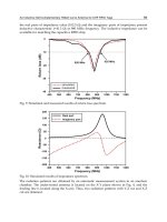
We have reported in Fig. 2 the value of Q(n, m) expressed by (5), as a function of the tree
level (i), for different values of the number of tags (n). As expected, the average number of
idle time slots quickly converges to the total number of time slots, that is, 2
i
.

0123456789101112131415
10
0
10
1
10
2
10
3

10
4
2
i
Q(50, 2
i
)
Q(100, 2
i
)
Q(200, 2
i
)
Q(300, 2
i
)
Q(400, 2
i
)
Q(500, 2
i
)
Idle Time Slots
Tree Level (i)

Fig. 2. Average number of idle time slots as a function of the tree level.
With similar arguments, we can consider that a time slot at level i is successful if it is used
by a single tag to reply to a query. So, the average number of successful time slots at the tree
level i can be estimated as follows:

( ) () ()
1
,1
n
Snm mnpm pm
−
=
⋅⋅ ⎡− ⎤
⎣
⎦
. (6)
Fig. 3 reports the average number of successful time slots as a function of the tree level, for
the same choices of the number of tags, calculated by means of (6). In this case, it is
immediate to observe that the number of successful time slots converges to the total number
of tags n.
Starting from the expressions (5) and (6) for Q(n, m) and S(n, m), respectively, the average
number of collisions at the tree level i can be estimated as the number of non-idle and non-
successful time slots, i.e.:

(
)
(
)
(
)
bin
,,,CnmmQnmSnm=− − . (7)
Radio Frequency Identification Fundamentals and Applications, Bringing Research to Practice

78

0123456789101112131415
10
0
10
1
10
2
10
3
S(50, 2
i
)
S(100, 2
i
)
S(200, 2
i
)
S(300, 2
i
)
S(400, 2
i
)
S(500, 2
i
)
Successful Time Slots
Tree Level (i)

Fig. 3. Average number of successful time slots as a function of the tree level.
Based on these considerations, it follows that the average number of time slots with
collisions rapidly goes to zero (a negative number of collisions obviously has no sense). For
better evidence, the average number of collisions, expressed by (7), is reported in Fig. 4, for
the same choices of n, as a function of the tree level. We observe that, for the initial tree
levels, the number of time slots with collisions coincides with the total number of time slots
(2
i
). Then, the number of collisions becomes smaller than 2
i
and, after reaching a maximum
value, begins to decrease monotonically.
The total number of collisions in the binary tree protocol can be found by summing the
average number of collisions at each tree level, that is:

()
()
bin bin
0
,2
i
i
Cn Cn
∞
=
=
∑
. (8)
The series surely converges because C
bin

(n, 2
i
) becomes null for the values of i exceeding a
given threshold. By substituting (5), (6) and (7), equation (8) can be rewritten as follows:

() ( )() ()
1
bin
0
11
nn
i
Cn m n pm npm
∞
−
=
⎡
⎤
=+− −⋅
⎣
⎦
∑
. (9)
Expression (9) allows to determine analytically the total number of collisions and, through
(3), we can then estimate the total number of time slots needed by the binary tree algorithm
to completely identifying the set of n tags. As we will see in the following, such analytical
estimation gives results that are very close to those of numerical simulations.
MAC Protocols for RFID Systems

79

0123456789101112131415
10
0
10
1
10
2
10
3
10
4
Collisions
Tree Level (i)
2
i
C(50, 2
i
)
C(100, 2
i
)
C(200, 2
i
)
C(300, 2
i
)
C(400, 2
i
)

C(500, 2
i
)

Fig. 4. Average number of time slots with collisions as a function of the tree level.
3. The framed slotted Aloha protocol
As we have seen in the previous section, the binary tree protocol for medium access control
in RFID systems exploits binary splitting of the tags into subgroups on the basis of their
identifiers, that are fixed and known a priori. For this reason, the binary tree and other
similar deterministic protocols are opposed to stochastic protocols, mostly based on the
framed slotted Aloha algorithm.
In slotted Aloha protocols, the time axis is divided into time slots. Each tag synchronizes its
transmission with the beginning of a time slot, in such a way that concurrent transmissions
collide completely. This is the main difference between slotted Aloha protocols and the pure
Aloha one, in which instead the time axis is not discretized, so partial collisions can occur as well.
In the framed version of the slotted Aloha protocol, time slots are grouped into groups of L,
and each group coincides with a frame. Each tag can transmit only once in each frame, and
frames are repeated until the end of the identification procedure.
At the beginning of a frame, each tag randomly selects a time slot within the frame for
transmitting its ID. The tag then transmits at the chosen time slot; if a collision occurs,
colliding tags wait the end of the current frame and repeat the procedure in the following
frame. The advantage of the introduction of frames is due to the limitation in the
transmission rate imposed by the fact that each tag only transmits once in a frame. This
allows to reduce the number of collisions in the initial phase of the protocol, when all tags
try to communicate. This can result in a significant performance improvement with respect
to slotted Aloha, on condition that the frame length is properly chosen.
Radio Frequency Identification Fundamentals and Applications, Bringing Research to Practice

80
In standard FSA, the frame length must be fixed a priori and is kept constant until

completion of the algorithm. When the number of tags significantly exceeds the frame size,
efficiency of the FSA protocol with fixed frames decreases. On the other hand, the algorithm
efficiency could be kept high by adjusting the frame length on the basis of the number of
active tags. In this case, however, such number must be estimated, that instead is not
necessary in classic FSA.
A first solution to the problem of estimating the number of tags in the FSA protocol is to
adopt dynamic versions of the FSA (Cha & Kim, 2005), (Lee et al., 2005). These approaches
exploit the dependence of the probability of collision on the frame size and the number of
tags. Such dependence can be expressed in analytical terms through theoretical arguments
similar to those used in the previous section for the analysis of the binary tree protocol.
Let P
idle
, P
succ
and P
coll
represent the probability that a time slot is idle, used for a successful
transmission or occupied by a collision, respectively. Similarly to (5) and (6), we can express
P
idle
and P
succ
as follows:

idle
1
succ
1
1
11

1
n
n
P
L
Pn
LL
−
⎧
⎛⎞
=−
⎪
⎜⎟
⎪⎝⎠
⎨
⎪
⎛⎞
=−
⎜⎟
⎪
⎝⎠
⎩
. (10)
Starting from (10), P
coll
can be calculated as:
P
coll
= 1 – P
idle

– P
succ
, (11)
so n can be estimated from the knowledge of L and the estimate of P
coll
. However, it has
been observed that the estimate of n so obtained can be inaccurate, since, for high values of
the collision probability, small errors in the estimation of P
coll
may produce significant
deviations of the estimated n from its actual value (Park et al., 2007).
Another important result that can be derived from (10) is that the optimal frame size in the
FSA algorithm exactly coincides with the number of tags n. So, FSA becomes less and less
efficient when the gap between L and n increases.
For this reason, in Dynamic FSA (DFSA), the probability of collision is used to obtain an
estimate of the number of tags that try to access the shared medium. This is repeated at each
frame, in such a way that the frame length is dynamically adjusted on the basis of the actual
number of contending tags. As anticipated, the estimated number of tags can be inaccurate.
We will denote by
α
the ratio between the estimated number of tags and its exact value
(thus,
α
= 1 represents the ideal behaviour).
3.1 FSA with robust estimation and binary selection
An efficient approach for estimating the number of contending tags in the FSA protocol has
been proposed in (Park et al., 2007), where the variant denoted as “FSA with Robust
Estimation and Binary Selection”, or EB-FSA, has been introduced.
The EB-FSA protocol begins with an estimation phase that has the purpose of estimating the
number of tags n and to adjust the frame size L consequently. The estimation phase

proposed in (Park et al., 2007) is robust, in the sense that it solves the issues due to high
sensitivity of the estimated n to estimation errors on P
coll
, in (11), for high values of the
collision probability.
MAC Protocols for RFID Systems

81
Estimation in EB-FSA starts by fixing an estimation frame size L
est
and a target P
coll
threshold
(P
coll-th
), that corresponds to a threshold number of tags (n
th
) through (10) and (11). The tag
reader estimates the value of n only when P
coll
becomes smaller than P
coll-th
, in such a way to
reduce inaccuracy on the estimate of n (n
est
). For this purpose, at each iteration of the
estimation phase, the tag reader reduces the number of tags polled by a factor f
d
, using a bit
mask in the query frame.

Estimation of the tags number is made only when P
coll
becomes smaller than P
coll-th
, i.e., after
a number of estimation frames equal to i
*
(n), that coincides with the smallest i such that
n/f
d
i-1
< n
th
. In formula:

()
th
1
*
1
arg max
i
d
i
i
d
n
n
f
n

in
f
−
−
∈
<
⎛⎞
=
⎜⎟
⎜⎟
⎝⎠

. (12)
Thus, in the EB-FSA protocol, the initial estimation phase requires I
est
= i
*
(n)L
est
time slots.
After such initial phase, tags randomly choose an integer between 1 and n
est
for transmission
of their ID, and a frame with length n
est
is transmitted. Differently from FSA, when a
collision occurs, colliding tags do not wait for the next frame to retransmit their ID. On the
contrary, a binary selection mechanism is implemented, that works as follows:
• non colliding tags increment their counters by 1;
• colliding tags randomly choose a binary value;

• colliding tags that chose 0 try retransmission at the next time slot;
• colliding tags that chose 1 try retransmission after one time slot;
• if another collision occurs, the procedure is repeated within the new set of colliding tags.
The binary selection mechanism avoids the need for subsequent frames, since each collision
is necessarily solved through the splitting procedure. The protocol succeeds when all the
tags have been identified, that is, after I
iden
time slots. So, the total number of time slots
needed by the EB-FSA protocol for completing its task is:
I
tot
= I
est
+ I
iden
= i
*
(n)L
est
+ I
iden
. (13)
As it will be evident through numerical simulations, the EB-FSA approach can achieve a
significant performance improvement with respect to FSA and DFSA.
4. Protocols comparison
In order to assess and compare the considered protocols for medium access control in RFID
systems, we report in this section the results of numerical simulations that model different
scenarios.
We are interested in estimating the time needed by the considered protocols to complete the
identification phase, in order to compare their efficiency in arbitrating the channel use in

groups of tags with different size. The actual identification speed depends on technology
issues, so we refer to the number of time slots instead of real time.
We consider, as a starting point, the classic implementation of the framed slotted Aloha
protocol, with fixed frame size. We consider two common values of frame size, that are L =
128 and L = 256, and estimate by simulation the total number of time slots needed to
complete the identification procedure (I
tot
). The results obtained are averaged over a number
of simulations sufficiently high to ensure a satisfactory level of statistic confidence.
Radio Frequency Identification Fundamentals and Applications, Bringing Research to Practice

82
0 50 100 150 200 250 300 350 400 450 500
0
200
400
600
800
1000
1200
1400
1600
1800
2000
2200
2400
2600
2800
I
tot

n
FSA (L = 128)
FSA (L = 256)
DFSA (α = 1)
DBT
Binary Tree (theor.)

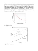
Fig. 5. Comparison of binary tree and framed slotted Aloha protocols.
The values of I
tot
, so obtained, are reported in Fig. 5 as a function of the total number of tags
(n). As we observe from the figure, the classic FSA protocol becomes less and less efficient
for an increasing number of tags. The curve corresponding to L = 128 exhibits a parabolic
behaviour starting from n on the order of 300. When L is increased up to 256, the protocol is
less efficient for a small number of tags (n between 0 and 350), but its performance is
improved for higher n. The parabolic behaviour of the curve for L = 256 is not apparent in
the figure, since occurs for higher values of n with respect to the simulation scope.
In Fig. 5, classic FSA is compared with Dynamic FSA, in which the frame length is changed
dynamically in such a way to coincide always with the number of contending tags. When
the estimation of the number of tags is exact ( = 1), the DFSA protocol is able to
significantly improve the performance of classic FSA. As we observe from the figure, the
improvement is on the order of 200 time slots with respect to FSA with L = 128 and n up to
250. When n increases, the advantage of adopting DFSA instead of FSA becomes more and
more relevant.
As an example of the binary tree algorithm, we consider a distributed binary tree (DBT)
protocol that is self-adjusting, and that is directly managed by tags (Baldi et al., 2008). It
recalls the classic version of the binary tree traversal, in which, when a collision occurs, each
client randomly chooses a binary value. This is the same principle at the basis of the binary
selection phase in the EB-FSA protocol. In DBT, the reader sends its query and all tags
randomly choose a binary value. Tags that chose 0 try transmission at the first time slot

available, while the others try transmission at the following time slot. If a collision occurs,
MAC Protocols for RFID Systems

83
the same procedure used in EB-FSA is adopted. So, colliding tags randomly select another
binary value, while all the others increment their counters by 1.
Such implementation of the BT protocol is independent of the bit coding of the tags IDs (that
instead must be suitably chosen in the RFID standard BT protocol). Moreover, a
fundamental role in RFID standard binary tree is played by the tag reader, that must
perform the splitting procedure based on the tags IDs. On the contrary, in DBT the tags are
able to manage the protocol autonomously, without the reader’s queries. This way, the tag
reader is not required to store the status of forked queries to avoid travelling each edge
more than once. On the other hand, a drawback of DBT is that it requires tags to perform
some processing (as for generation of pseudo-random binary values), so it could be difficult
to implement with passive tags.
As we see from Fig. 5, performance of the DBT protocol is very close to the theoretical
expectation, expressed by (9). DBT is able to improve significantly the performance of
standard FSA and, for a number of tags up to 500, gives a moderate performance loss with
respect to DFSA.
As a further assessment, we can compare the performance of the DBT protocol with that of
EB-FSA. A simple example of application of the two protocols is reported in Fig. 6, where
we consider the case of n = 5 tags. We observe from the figure that the only difference
between the two protocols consists in the distribution of the initial values of the tag
counters: in EB-FSA each tag must know the frame size (L = 5, in this case) and chooses its
random value accordingly. In DBT, instead, each tag starts by choosing a binary value,
without any knowledge on the frame size. However, even without needing any information
on the number of tags, the DBT protocol is able to achieve the same performance as the EB-
FSA, in the considered example, since both protocols complete identification in 8 time slots.
Moreover, contrary to EB-FSA, DBT does not require any estimation phase before
identification.

On the other hand, it should be observed that the DBT protocol produces a higher number
of collisions with respect to EB-FSA, due to the fact that the initial values chosen by the tags
are only binary. In EB-FSA, instead, tags can select initial values in the range between 1 and
n
est
. For these reasons, the DBT protocol is less efficient than EB-FSA under the power
consumption viewpoint.

DBT EB-FSA
Counte
r
12121010
Counter
210100
Tag1 C S Tag1 C C S
Counte
r
01010
Counter
0
Tag2 C C S Tag2 S
Counte
r
0100
Counter
2101010
Tag3 C C S Tag3 C C S
Counte
r
1212100

Counter
2100
Tag4 C S Tag4 C S
Counte
r
00
Counter
32121210
Tag5 C S Tag5 S
Time Slot
12345678
Time Slot
12345678

Fig. 6. Example of application of DBT and EB-FSA protocols.
When the number of tags increases, the advantage of having many possible initial random
values in EB-FSA becomes more and more relevant, yielding a performance improvement
Radio Frequency Identification Fundamentals and Applications, Bringing Research to Practice

84
with respect to the DBT protocol. This is shown in Fig. 7, where DBT is compared with EB-
FSA through numerical simulations, for a number of tags up to 500.
As we observe from the figure, under the hypothesis of perfect estimation of the number of
tags, the EB-FSA protocol outperforms the DBT one. However, we can take into account the
number of time slots needed by the initial estimation phase of EB-FSA, I
est
, calculated on the
basis of (12). The value of I
est
has been found by considering, for the estimation phase, the

same choice of the parameters proposed in (Park et al., 2007), that is, L
est
= 64, P
coll-th
= 0.7
and f
d
= 4. By considering the estimation phase, the performance gain achieved by EB-FSA
becomes smaller and the two protocols have almost the same performance for a number of
tags up to 300. So, the DBT protocol could still represent a valid choice, since it does not
require the initial estimation phase, that has some drawbacks under the complexity
viewpoint.

0 50 100 150 200 250 300 350 400 450 500
0
100
200
300
400
500
600
700
800
900
1000
1100
1200
1300
1400
1500

EB-FSA (α = 1) w/o est.
EB-FSA (α = 1)
DBT
I
tot
n

Fig. 7. Comparison of DBT and EB-FSA with perfect estimation ( = 1).
Another important aspect that must be taken into consideration is that, in the EB-FSA
protocol, the estimation phase could be inaccurate, so the performance gain with respect to
DBT could be further reduced.
We consider two different cases, in which we suppose that the reader estimates a number of
tags equal to 0.5 and 1.5 times the actual number. The results of numerical simulations of the
EB-FSA protocol with inaccurate estimation are reported in Fig. 8, where they are compared
with those of the DBT algorithm.
MAC Protocols for RFID Systems

85
We observe that the DBT protocol achieves almost the same performance as the EB-FSA in
both the considered cases with inaccurate estimation. The overhead due to the initial
estimation phase in EB-FSA has been also taken into account.
So, for a number of tags up to 500 (that is of interest for many applications), the DBT
protocol (or, equivalently, the binary tree protocol based on tags IDs) is able to guarantee a
rather good collision arbitration. Its performance compares with that of optimized stochastic
algorithms, as the EB-FSA.
However, as we notice from the figure, the DBT curve has a higher slope with respect to
those of EB-FSA and intersects them at n ≈ 300. This confirms that, when the number of tags
increases, the advantage of EB-FSA becomes more and more relevant.

0 50 100 150 200 250 300 350 400 450 500

0
100
200
300
400
500
600
700
800
900
1000
1100
1200
1300
1400
1500
EB-FSA (α = 0.5)
EB-FSA (α = 1.5)
DBT
I
tot
n

Fig. 8. Comparison of DBT and EB-FSA with inaccurate estimation ( = 0.5, 1.5).
5. Conclusion
A very common requirement in RFID systems is the reading of co-located tags, that is
necessary when multiple tags are found simultaneously in the coverage area of the tag
reader. Due to the low latency and low power constraints of these systems, the availability
of efficient protocols able to arbitrate collisions and guarantee shared access to the
transmission medium becomes of fundamental importance.

This chapter has described several anti-collisions protocols for RFID systems, that can be
grouped in the two main categories of deterministic and stochastic protocols. We have seen
that deterministic protocols, as the binary tree algorithm, can outperform classic stochastic
Radio Frequency Identification Fundamentals and Applications, Bringing Research to Practice

86
protocols as the framed slotted Aloha with fixed frame length. By considering more efficient
versions of stochastic protocols, like the Dynamic FSA and the EB-FSA, the performance in
terms of identification speed can be improved in a significant manner.
All these protocols, however, require estimation of the number of contending tags. So, the
BT algorithm could still represent a good solution for resolving collisions without the need
of tags estimation. We have seen that the BT protocol can also be implemented in a
distributed manner, in such a way to be managed directly by tags and to be independent of
the bit coding of the tags identifiers. This could represent an alternative to the RFID
standard BT protocol (with centralized coordination) when intelligent tags are available.
6. References
Baldi, M., Morichetti, S. & Gambi, E. (2008). “A distributed binary tree protocol for medium
access control in RFID systems”, in Proc. SoftCOM 2008, Split, Dubrovnik, Croatia,
25-27 Sep. 2008, pp. 228-232.
Cappelletti, F., Ferrari, G. & Raheli, R. (2006). “A simple performance analysis of multiple
access RFID networks based on the binary tree protocol”, in Proc. Intern. Symp.
Commun. Control Signal Proc. (ISCCSP '06), Marrakech, Morocco, Mar. 2006.
Cha, J R. & Kim, J H. (2005). “Novel Anti-Collision Algorithms for Fast Object
Identification in RFID Systems”, in Proc. ICPADS 2005, Fukuoka, Japan, Jul. 2005,
vol. 2, pp. 63–67.
Feng, B., Li, J T., Guo, J B. & Ding, Z H. (2006). “ID-Binary Tree Stack Anticollision
Algorithm for RFID”, in Proc. IEEE ISCC '06, Cagliari, Italy, Jun. 2006, pp. 207–212.
ISO/IEC 18000–6 (2003). “Information technology automatic identification and data capture
techniques - radio frequency identification for item management air interface – part
6: parameters for air interface communications at 860-960 MHz”, Nov. 2003.

Janssen, A. & De Jong, M. (2000). “Analysis of Contention Tree Algorithms”, IEEE Trans.
Inform. Theory, vol. 46, no. 6, pp. 2163–2172.
Lee, S R., Joo, S D. & Lee, C W. (2005). “An Enhanced Dynamic Framed Slotted ALOHA
Algorithm for RFID Tag Identification”, in Proc. MobiQuitous 2005, San Diego, CA,
Jul. 2005, pp. 166–172.
Myung, J., Lee, W. & Srivastava, J. (2006). “Adaptive Binary Splitting for Efficient RFID Tag
Anti-Collision”, IEEE Commun. Lett., vol. 10, no. 3, pp. 144–146.
Namboodiri, V. & Gao, L. (2007). “Energy-Aware Tag Anti-Collision Protocols for RFID
Systems”, in Proc. IEEE PerCom '07, White Plains, NY, Mar. 2007, pp. 23–36
Park, J., Chung, M. Y. & Lee, T J. (2007). “Identification of RFID Tags in Framed-Slotted
ALOHA with Robust Estimation and Binary Selection”, IEEE Commun. Lett., vol. 11,
no. 5, pp. 452–454, May 2007.
Want, R. (2006). “An Introduction to RFID Technology”, IEEE Perv. Comput., vol. 5, no. 1, pp.
25-33.
6
Stochastical Model and Performance Analysis
of Frequency Radio Identification
Yan Xinqing
1
, Yin Zhouping
2
and Xiong Youlun
2

1
School of Information Engineering, North China University of
Water Conservancy and Electric Power,
2
State Key Laboratory of Digital Manufacturing Equipment and Technology,
Huazhong University of Science and Technology,

China
1. Introduction
RFID (Radio Frequency Identification) can assign a unique digital identifier to each physical
item, and provide an efficient, cheap and contactless method for gathering the information
of the physical items to enable their automatic tracking and tracing(Finkenzeller 2003). RFID
technology serves as the back stone of the “Internet of Things”(Engels 2001), and is
reviewed as a main enabler of the upcoming “Pervasive Computing”(Stanford 2003). RFID
systems have been widely adopted in quite a lot applications, ranged from “smart box” to
world-wide logistics management systems.
A typical RFID system is consisted of some RFID tags, one or more RFID readers and the
backend information system. Each RFID tag holds a unique identifier and is attached to a
physical item. RFID reader is used to collect the identifiers stored in the RFID tags located in
its vicinity and is often connected with the backend information system. During
identification, The RFID reader asks the RFID tags to modulate their binary identifiers into
signals and transmit these signals back to the reader through the air interface, which is a
wireless communication channel for the RFID tag and reader to exchange information.
Afterwards, The RFID reader sends the data gathered to the backend information system for
further processing and dispatching to various applications.
One of the main issues that affect the universal deployment and application of the RFID
system is the collisions occurred during RFID tag identification(Wu 2006). The simultaneous
modulated signals broadcasted by the RFID reader and transmitted from the RFID tags will
interfere in the air interface, in which case, what the receivers can get is only a collision
signal but no useful information. Collisions occurred in the RFID system can be categorized
as the reader-reader, reader-tag and tag-tag collisions(Shih 2006).
When two or more RFID readers try to broadcast messages through the air interface
simultaneously, reader-reader collision occurs. Due to that they are often connected with the
computer system and can be equipped with enough resource to monitor the air interface,
RFID readers can detect the collision and coordinate with each other in advance. Reader-
reader collision can be avoided and resolved completely with some deliberate designed
protocols, such as the ColorWav(Waldrop 2003) and others(Leong 2006).

Radio Frequency Identification Fundamentals and Applications, Bringing Research to Practice
88
Reader-tag collision can also be avoided easily by asking the RFID reader and RFID tags to
broadcast message and transmit identifiers in different time, so that the signals broadcasted
by the RFID reader and transmitted from RFID tags will never collide in the air interface
and reader-tag collision will never occur.
When two or more RFID tags try to transmit their identifiers simultaneously through the air
interface, tag-tag collision will occur. Due to the extreme constraints on computation,
communication and energy supply put on RFID tags, especially that in passive RFID
system, RFID tag can only get power supply through the reflection of the waveforms
broadcasted by the RFID reader, tag-tag collision cannot be resolved easily using existed
collision resolution methods, such as CDMA (Code Division Multi Access), FDMA
(Frequency Division Multi Access), SDMA (Space Division Multi Access) and TDMA (Time
Division Multi Access), proposed in other communication systems(Theodore 2006).
Proposed protocols for RFID tag collision resolution can be classified as the probabilistic
frame slotted ALOHA based protocols, the deterministic splitting tree based protocols, and
some hybrid protocols, such as the slotted tree protocol (Bonuccelli 2007). The deterministic
splitting tree based RFID tag collision resolution protocols suffer from scalability, and
perform clumsily in resolving the collision caused by a large amount of RFID tags, while the
hybrid protocols are seldom adopted in real RFID systems, so these collision resolution
protocols will not be discussed any further in this chapter.
Due to that in a frame, each RFID tag can only choose a slot to transmit its data, the RFID tag
collision resolution process using the frame slotted ALOHA based protocols can be viewed as
a binomial distribution process, the identification accuracy and the efficiency of the protocol
depends seriously on the estimation and choice of some key parameters.
In this chapter, for the probabilistic frame slotted ALOHA based RFID tag collision
resolution protocol, based on the binomial distribution model, the accurate estimation of the
RFID tag population and the optimal choice some key parameters adopted in the collision
resolution protocol are analyzed, the Markov chain and its corresponding transition matrix
for RFID tag collision resolution are proposed to determine the amount of frames needed in

the identification, and our research is verified by numeric simulations.
The remaining sections of this chapter is organized as follows: section 2 presents the basic
assumption we hold in this chapter and reviews briefly the frame slotted ALOHA based
RFID tag collision resolution protocols. Section 3 discusses the stochastical distribution
model for RFID tag collision resolution based on the binomial distribution and the Markov
chain, and some key parameters that affect the performance of the collision resolution
protocol are analyzed. Section 4 describes and analyzes the result of the numeric simulations
performed to verify our research. And finally in Section 5, we conclude.
2. Basic assumptions and the frame slotted ALOHA based protocols
2.1 Basic assumptions
In this chapter, as presented in (Kaplan 1985) for the analysis of multiple-access protocols,
we hold the following basic conventions in the discussions:
• Time is slotted, each time slot can be either a command slot for the RFID reader to
broadcast a message or a data slot for the RFID tags to transmit their binary identifiers.
• One RFID tag group is interrogated in a data slot.
• The air interface is perfect, and no signal transmission error or lose occurs in it.
• The air interface is ternary, the interrogation of a tag group reveals the presence of zero,
one and two or more RFID tags.
Stochastical Model and Performance Analysis of Frequency Radio Identification
89
But unlike (Kaplan 1985), in this chapter, it is assumed that the air interface is instantaneous,
not delayed, due to the limited distance between the RFID reader and RFID tags. However,
short time intervals are needed for the RFID reader and tags to modulate and transfer a bit
through the air interface. As other research work on RFID tag collision resolution protocols,
it is assumed that RFID tags remain stable in a collision resolution cycle, neither newly
arrived RFID tag enters nor does existed RFID tags leave the interrogation zone of the RFID
reader during an identification cycle.
2.2 The frame slotted ALOHA based RFID tag collision resolution protocols
The ALOHA protocol for resolving the collision occurred in wireless communication was
originally proposed by N. Abramson from the Hawaii University in the 1970s to enable the

terminals distributed in isolated islands to exchange information with the mainframe
computer system(Abramson 1970). In this protocol, each terminal can choose a time interval
randomly to transmit its data to the mainframe, and if the time interval is occupied solely by
the terminal, the data can be received by the mainframe successfully. Otherwise, if the time
interval is occupied by two or more terminals and collapses, the data signals from these
terminals will interfere, and collision will occur, and each terminal is acknowledged with
the collision and will choose randomly another time interval afterward for retransmission.
An improvement of the ALOHA protocol is the slotted ALOHA protocol (Roberts 1975), in
which the time is slotted, each terminal can only choose randomly a whole time slot, start data
transmission at the beginning of the time slot and finish transmission at the end of it. In such a
way, a lot of collisions occurred in the wireless communication channel can be avoided.
Due to its simplicity and easiness of implementation, the slotted ALOHA protocol was
introduced to the RFID system to resolve the tag-tag collisions, which are caused by that
two or more RFID tags try to transmit their identifiers simultaneously through the air
interface, and various frame slotted ALOHA based RFID tag collision resolution protocol
have been suggested, such as the standard frame slotted ALOHA protocol, the dynamic
frame slotted ALOHA protocol, the extended frame slotted ALOHA protocol and etc. Some
frame slotted ALOHA protocols have been adopted as international or industrial standards.
In all these protocols, the overall process that a RFID reader tries to collect the identifiers
stored in the RFID tags within its vicinity is called a collision resolution cycle (or an
identification cycle), which is consisted of a series of frames. And in each frame there is a
command slot and a series of data slots.
In the command slot of a frame, the RFID reader broadcasts a command message to RFID
tags in its interrogation zone to indicate the number of data slots (frame length), s, adopted
in this frame. Each RFID tag, upon receiving this message and decoding the frame length s,
randomly generates an integer i in the range 0 s-1, modulates its binary identifier into
signals and transmits the signals back to the RFID reader in the ith data slot through the air
interface. Due to the constraint on computation put on RFID tags, s is often chosen as a
integer mean of 2 and in the range [2,4,8,16,32,64,128,256].
Afterwards, the RFID reader gathers information contained in the data slots of the frame. If in

a data slot, no RFID tag chooses to transmit its identifier, the data slot is called an idle slot. Else
if in a data slot, there is one and only one RFID tag choosing to transmit its identifier, the data
slot is called a success slot, the identifier is gathered and the RFID tag is identified successfully.
Otherwise, two or more RFID tags choose to transmit their identifiers in the data slot, collision
will occur and the data slot is called a collision slot, in such case, what the RFID reader can get
is only a collision signal but no other useful information.
Radio Frequency Identification Fundamentals and Applications, Bringing Research to Practice
90
If after a frame, the desired identification accuracy of RFID tags specified by the application
system is achieved, the current collision resolution cycle can be terminated, and the RFID
reader will report the result to the backend information system for further processing and
dispatching. Otherwise, another collision resolution frame is needed, and the same
identification process is repeated.
3. The stochastical model for collision resolution of RFID tags
3.1 The binomial distribution model for RFID tag collision resolution
In a collision resolution frame, due to that each RFID tag can only randomly choose one data
slot to transmit its digital identifier, this procedure can be viewed as a typical binomial
distribution process.
Suppose that the population of RFID tags within the vicinity of the RFID reader is t and the
frame length is s, the probability that n RFID tags choose a common data slot to transmit
their identifiers can be calculated with the binomial distribution as

,






1




1 
1




(1)
where 



!
!



!
. And the mathematical expects of this binomial distribution can be
calculated with

,










1



1 
1




(2)
Suppose that 

is a random variable representing the amount of data slots that r RFID tags
chooses the data slot to respond, where r∈[0,1, ,t-1], the distribution of 

, according to
(Feller 1970), is












∏





,






(3)
where 

,

 


∑
1

∏







!








.
The mathematical expects for the number of idle, success and collision data slots, 
,,
, 
,,
,
and 
,,
achieved in the frame can be calculated as

,,
1
1










,,
1
1



 





,,

,,

,,
11







(4)

The values of 
,,
, 
,,
and 
,,
for the identification of different amount of RFID tags
with fixed frame length s=256 are shown in Fig. 1. From Fig. 1, it can been observed that for
the collision resolution protocol with fixed frame length, as tag population increases, the
amount of collision slots also increases rapidly and approaches to the frame length, and the
Stochastical Model and Performance Analysis of Frequency Radio Identification
91
amount of idle slots deacreses rapidly and approaches to 0, while the amount of success
slots, after reaches a maximum value, will also decrease rapidly and approach to 0 finally.

Fig. 1. The Values of 
,,
, 
,,
and 
,,
for Different Tag Population and Fixed Frame
Length s=256
3.2 Estimation of RFID tag population
In typical RFID applications, the population of RFID tags within the vicinity of the RFID
reader is usually unknown in advance. For the frame slotted ALOHA based RFID tag
collision resolution protocols, accurate estimation of the RFID tag population is a necessity
for the calculation of the identification accuracy achieved after a frame and the termination
of the current collision resolution cycle.
Proposed methods for the estimation of the RFID tag population adopted in the frame

slotted ALOHA based protocols, according to the name of the proposer, can be categorized
as the Vogt-1, the Zhen-1, the Cha-1, the Cha-2 and the Vogt-2 methods.
The Vogt-1 method (Vogt 2002) refers to that after an identification frame, if the amounts of
idle, successful and collision slots are a
0
, a
1
, and a
k
, due to that a
1
RFID tags respond in the
successful slots and that every collision is occupied by the identifiers from at least 2 RFID
tags, the overall population of RFID tags that respond in the frame can estimated as t
directly with


2

(5)
The Zhen-1 method (Zhen 2005) uses the probability that collision occurs in a data slot to
estimate the overall population of RFID tags in the vicinity of the RFID reader. The
probability that a RFID tag may collide with other RFID tags in a data slot can be calculated
as
Radio Frequency Identification Fundamentals and Applications, Bringing Research to Practice
92



1


1
1 
1



1


1 
1




(6)
where 

and 

refer to probabilities that a data slot result in collision and success.
According to the law of large number, the stable of value of  can be achieved when t∞,
and in such case, C can be calcuated as C=0.418. So the overall population of RFID tags that
transmits their identififers in the frame can be estimated with









 2.392


(7)
Another method proposed in (Cha 2005) is that the overall population of RFID tags within
the vicinity of the RFID reader should be estimated as t=2.392a
k
, and this method is called
the Cha-1 in this chapter.
As proposed in (Cha 2006) according to the binomial distribution of the frame slotted
ALOHA based RFID tag collision resolution protocols, the mathematical expects for the
amounts of idle, successful and collision slots can be calculated with Eq. 3, if after a frame,
the actual number of collision slots is a
k
, for the equation 

 11






, for known
s, the value of t can be calcuated with the Newton or other literation methods.
This calculation is time consuming, so to ease the calculation, for the framel length s adopted
in the protocol, we can calcuated the value of 

,,
for different t, and compare a
k
with it to
find the approximate RFID tag population t. That is, through seaching t to minize the



,,
, the appropriate value of RFID tag population can be founded. This method is
called Cha-2, and also has been proposed in (Kodialam 2006).
It should be noticed that the search range of t should be limited to [a
1
+2a
k
, 2(a
1
+2a
k
)], for that
(a
1
+2a
k
) is the low limit of the tag population, and numeric simulation presented in section 4
shows that the chance is rare for actual RFID tag population exceeds 2(a
1
+2a
k
).

As proposed in (Vogt 2002), accroding to the Chebyshev's inequality, the result for random
experiment with random variable X is most likely results in the mathematical expects of X,
and to resolve the collision caused by different number of RFID tags t with frame length s,
the mathematical expects of 
,,
, 
,,
and 
,,
achieved in a frame can be calculated in
advance. And if after the frame, if the actual amounts of idle, success and collision slots are
a
0
, a
1
, and a
k
, the population of RFID tags t can be calculated by minimizing the difference
between the tuples < a
0
, a
1
, a
k
,> and <
,,
, 
,,
, 
,,

>. That is to find the RFID tag
population t, which satisfies






,,



,,



,,



(8)
The search range of RFID tag population t can also be limited to the range [(a
1
+2a
k
),
2(a
1
+2a
k

)], as discussed above.
These methods estimate the population of RFID tags within the interrogation zone of the
RFID reader from different views, and the estimation accuracy achieved in each method
needs to be examined with further numeric simulations.