Engineering - Materials Selection in Mechanical Design Part 3 pdf

Engineering materials and their
properties
3.1
Introduction and synopsis
Materials, one might say, are the food of design. This chapter presents the menu: the full shopping
list of materials. A successful product
-
one that performs well, is good value for money and
gives pleasure to the user
-
uses the best materials for the job, and fully exploits their potential
and characteristics: brings out their flavour,
so
to speak.
The classes of materials
-
metals, polymers, ceramics, and
so
forth
-
are
introduced in
Section
3.2.
But it is not, in the end, a material that we seek; it is a certain profile of properties.
The properties important in thermo-mechanical design are defined briefly in Section
3.3.
The reader
confident in the definitions of moduli, strengths, damping capacities, thermal conductivities and the
like may wish to
skip

this, using it for reference, when needed, for the precise meaning and units
of the data in the selection charts which come later. The chapter ends, in the usual way, with a
summary.
3.2
The classes
of
engineering material
It
is conventional to classify the materials
of
engineering into the six broad classes shown in
Figure
3.1
:
metals, polymers, elastomers, ceramics, glasses and composites. The members of a
class have features in common: similar properties, similar processing routes, and, often, similar
applications.
Metals have relatively high moduli. They can be made strong by alloying and by mechanical
and heat treatment, but they remain ductile, allowing them to be formed by deformation processes.
Certain high-strength alloys (spring steel, for instance) have ductilities as low as
2%,
but even this
is enough to ensure that the material yields before it fractures and that fracture, when it occurs, is
of a tough, ductile type. Partly because of their ductility, metals are prey to fatigue and of all the
classes of material, they are the least resistant to corrosion.
Ceramics and glasses, too, have high moduli, but, unlike metals, they
are
brittle. Their ‘strength’
in tension means the brittle fracture strength; in compression it is the brittle crushing strength,
which is about

15
times larger. And because ceramics have no ductility, they have a low tolerance
for stress concentrations (like holes or cracks) or for high contact stresses (at clamping points,
for instance). Ductile materials accommodate stress concentrations by deforming in a way which
redistributes the load more evenly; and because of this, they can be used under static loads within
a small margin of their yield strength. Ceramics and glasses cannot. Brittle materials always have
Engineering materials and their properties
21
Fig.
3.1
The menu
of
engineering materials.
a wide scatter in strength and the strength itself depends on the volume of material under load and
the time for which
it
is applied.
So
ceramics are not as easy to design with as metals. Despite this,
they have attractive features. They are stiff, hard and abrasion-resistant (hence their use for bearings
and cutting tools); they retain their strength to high temperatures; and they resist corrosion well.
They must be considered as an important class of engineering material.
Polymers
and
elastomers
are at the other end of the spectrum. They have moduli which are low,
roughly
SO
times less than those of metals, but they can be strong
-

nearly as strong as metals. A
consequence of this is that elastic deflections can be large. They creep, even at room temperature,
meaning that a polymer component under load may, with time, acquire a permanent set. And their
properties depend on temperature
so
that a polymer which is tough and flexible at
20°C
may be
brittle at the
4°C
of a household refrigerator, yet creep rapidly at the
100°C
of boiling water. None
have useful strength above
200°C.
If these aspects are allowed for in the design, the advantages of
polymers can be exploited. And there are many. When combinations of properties, such as strength-
per-unit-weight, are important, polymers are as good as metals. They are easy to shape: complicated
parts performing several functions can be moulded from a polymer in a single operation. The large
elastic deflections allow the design of polymer components which snap together, making assembly
fast and cheap. And by accurately sizing the mould and pre-colouring the polymer, no finishing
operations are needed. Polymers are corrosion resistant, and they have low coefficients
of
friction.
Good design exploits these properties.
Composites
combine the attractive properties of the other classes of materials while avoiding some
of their drawbacks. They are light, stiff and strong, and they can be tough. Most of the composites at
present available to the engineer have a polymer matrix
-

epoxy or polyester, usually
-
reinforced
by fibres of glass, carbon or Kevlar. They cannot be used above
250°C
because the polymer matrix
softens, but at room temperature their performance can be outstanding. Composite components are
expensive and they are relatively difficult to form and join.
So
despite their attractive properties the
designer will use them only when the added performance justifies the added cost.
22
Materials Selection in Mechanical Design
The classification of Figure 3.1 has the merit of grouping together materials which have some
commonalty in properties, processing and use. But it has its dangers, notably those of specialization
(the metallurgist who knows nothing of polymers) and of conservative thinking ('we shall use steel
because we have always used steel'). In later chapters we examine the engineering properties of
materials from a different perspective, comparing properties across all classes of material. It is the
first step
in
developing the freedom of thinking that the designer needs.
3.3
The definitions of material properties
Each material can be thought
of
as having a set of attributes: its properties. It is not a material,
per se,
that the designer seeks;
it
is a specific combination of these attributes: a

property-profile.
The material name is the identifier for a particular property-profile.
The properties themselves are standard: density, modulus, strength, toughness, thermal conduc-
tivity, and so on (Table
3.1).
For
completeness and precision, they are defined, with their limits, in
this section. It makes tedious reading. If you think you know how properties are defined, you might
jump to Section 3.4, returning to this section only if the need arises.
The
densiQ,
p
(units: kg/m3), is the weight per unit volume. We measure it today as Archimedes
did: by weighing
in
air and in a fluid of known density.
The
elastic modulus
(units: GPa or GN/m2) is defined as 'the slope of the linear-elastic part of
the stress-strain curve' (Figure
3.2).
Young's modulus,
E,
describes tension or compression, the
shear modulus
G
describes shear loading and the bulk modulus
K
describes the effect of hydrostatic
pressure. Poisson's ratio,

v,
is dimensionless: it is the negative of the ratio of the lateral strain to the
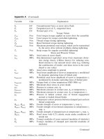
Table
3.1
Design-limiting material properties and their usual
SI
units*
Class
Property
Symbol
and
units
General
Mechanical
Thermal
Wear
Corrosion/
Oxidation
cost
Density
Elastic moduli (Young's, shear, bulk)
Strength (yield, ultimate, fracture)
Toughness
Fracture toughness
Damping capacity
Fatigue endurance limit
Thermal conductivity
Thermal diffusivity
Specific heat
Melting point

Glass temperature
Thermal expansion coefficient
Thermal shock resistance
Creep resistance
Archard wear constant
Corrosion rate
Parabolic rate constant
kA
kP
K
*Conversion factors to imperial and cgs
units
appear inside the back and front covers
of
this book.
Engineering materials and their properties
23
Fig.
3.2
The stress-strain curve for a metal, showing the modulus,
E,
the
0.2%
yield strength,
ay,
and
the ultimate strength
0,.
axial strain,
~21~1,

in axial loading. In reality, moduli measured
as
slopes of stress-strain curves
are inaccurate (often low by
a
factor of two or more), because of contributions to the strain from
anelasticity, creep and other factors. Accurate moduli are measured dynamically: by exciting the
natural vibrations of
a
beam or wire, or by measuring the velocity of sound waves in the material.
In
an isotropic material, the moduli are related in the following ways:
E E
G=-
K=
(3.1)
3G
E=
1
+
G/3K
2(1
+
u)
3(1
-
2~)
(3.2a)
1
1

Commonly
ux
113
when
G
x
3/8E
and
.K
%E
Elastomers are exceptional. For these:
(3.2b)
u=
112
when G
=
1/3E
and
K
>>
E
Data books and databases like those described in Chapter 13 list values for all four moduli. In this
book we examine data for E; approximate values for the others can be derived from equations (3.2)
when needed.
The
strength,
af,
of
a
solid (units: MPa or MN/m2) requires careful definition. For metals, we

identify
of
with the 0.2% offset yield strength
av
(Figure 3.2), that is, the stress at which the
stress-strain curve for axial loading deviates by
a
strain of 0.2% from the linear-elastic line. In
metals it is the stress at which dislocations first move large distances, and is the same in tension and
compression. For polymers,
af
is identified as the stress
a?
at which the stress-strain curve becomes
markedly non-linear: typically, a strain of
1
%
(Figure
3.3).
This may be caused by ‘shear-yielding’:
the irreversible slipping of molecular chains; or it may be caused by ‘crazing’: the formation of
low density, crack-like volumes which scatter light, making the polymer look white. Polymers are a
little stronger (~20%) in compression than in tension. Strength, for ceramics and glasses, depends
strongly on the mode of loading (Figure 3.4). In tension, ‘strength’ means the fracture strength,
0;.
24
Materials Selection in Mechanical Design
Fig.
3.3
Stress-strain curves for a polymer, below, at and above its glass transition temperature,

T,.
~~
c-T
Fig.
3.4
Stress-strain curves for a ceramic in tension and in compression. The compressive strength
a,
is
10
to
15
times greater than the tensile strength
at.
Fig.
3.5
The modulus-of-rupture (MOR) is the surface stress at failure in bending.
It
is equal to, or slightly
larger than the failure stress in tension.
In
compression it means the crushing strength
a;
which is much larger; typically
a;
=
10
to
15
x
0;

(3.3)
When the material is difficult to grip (as is a ceramic), its strength can be measured in bending. The
modulus
ofrupture
or
MOR
(units: MPa or MN/m2) is the maximum surface stress in a bent beam
at the instant of failure (Figure
3.5).
One might expect this to be exactly the
same
as the strength
Engineering materials and their properties
25
measured in tension, but for ceramics it is larger (by
a
factor of about
1.3)
because the volume
subjected to this maximum stress is small and the probability
of
a large flaw lying in it is small
also; in simple tension all flaws see the maximum stress.
The strength of
a
composite is best defined by
a
set deviation from linear-elastic behaviour:
0.5%
is

sometimes taken. Composites which contain fibres (and this includes natural composites
like wood) are a little weaker (up to
30%)
in compression than tension because fibres buckle.
In
subsequent chapters,
af
for composites means the tensile strength.
Strength, then, depends on material class and on mode of loading. Other modes of loading are
possible: shear, for instance. Yield under multiaxial loads are related to that in simple tension by
a
yield function, For metal5, the Von Mises yield function is
a
good description:
(3.4)
2 2
2
2
(a1
-
ff2)
+
(ff2
-
(73)
+
(03
-
ffl)
=

20f
where
01,
a2
and
03
are the principal stresses, positive when tensile;
01,
by convention, is the largest
or most positive,
03
the smallest
or
least. For polymers the yield function is modified to include the
effect of pressure
where
K
is
the bulk modulus of the polymer,
B
(~2)
is a numerical coefficient which characterizes
the pressure dependence of the flow strength and the pressure
p
is defined by
1
3
p
=
(01

+
ff2
+
03)
For ceramics,
a
Coulomb flow law is used:
where
B
and
C
are constants.
The
ultimate (tensile) strength
a,
(units:
MPa)
is the nominal stress at which
a
round bar of the
material, loaded in tension, separates (Figure
3.2).
For brittle solids
-
ceramics, glasses and brittle
polymers
-
it is the same
as
the failure strength in tension. For metals, ductile polymers and most

composites, it is larger than the strength
af,
by
a
factor of between
1.1
and
3
because
of
work
hardening or (in the case of composites) load transfer to the reinforcement.
The
resilience,
R
(units: J/m3), measures the maximum energy stored elastically without any
damage to the material, and which
is
released again on unloading. It is the area under the elastic
part of the stress-strain curve:
where
modulus. Materials with large values
of
R
make good springs.
is the failure load, defined
as
above,
Ej
is

the corresponding strain and
E
is Young’s
The
hardness,
H,
of
a
material (units: MPa) is a crude measure
of
its strength. It is measured
by
pressing
a
pointed diamond or hardened steel ball into the surface of the material. The hardness is
defined as the indenter force divided by the projected area
of
the indent. It
is
related to the quantity
26
Materials Selection in Mechanical Design
we
have defined as
af
by
H
2
3(~f
(3.7)

Hardness is often measured in other units, the commonest
of
which is the Vickers
H,
scale with
units
of
kg/mm2. It
is
related to
H
in the units used here by
H
=
IOH,
The
zoughness,
G,
(units: kJ/m2), and the
fracture
toughness,
K,
(units: MPam’/2 or MN/m’/’)
measure the resistance
of
the material
to
the propagation of a crack. The fracture toughness is
measured by loading a sample containing a deliberately introduced crack of length
2c

(Figure
3.6),
recording the tensile stress
(T,
at which the crack propagates. The quantity
K,
is then calculated
from
(3.8)
0,
K,
=
Y-
fi
K:
and the toughness from
(3.9)
Gc
=
E(l
+
v)
where
Y
is
a geometric factor, near unity, which depends on details of the sample geometry,
E
is Young’s modulus and
v
is Poisson’s ratio. Measured in this way

K,
and
G,
have well-defined
values for brittle materials (ceramics, glasses, and many polymers). In ductile materials a plastic
zone develops at the crack tip, introducing new features into the way in which cracks propagate
which necessitate more involved characterization. Values for
K,
and
G,
are, nonetheless, cited, and
are useful as a way
of
ranking materials.
The
loss-coeflcient,
q
(a dimensionless quantity), measures the degree to which a material dissi-
pates vibrational energy (Figure
3.7).
If
a material is loaded elastically to a stress
(T,
it stores an
elastic energy
.=.i
2E
“max
102
(TdE

=

per unit volume.
If
it is loaded and then unloaded, it dissipates an energy
AU=
odE
/
Fig.
3.6
The fracture toughness,
Kc,
measures the resistance
to
the propagation of a crack. The failure
strength of a brittle solid containing a crack
of
length
2c
is
of
=
YKCG
where
Y
is a constant near unity.
Engineering materials and their properties
27
Fig.
3.7

The
loss
coefficient
q
measures the fractional energy dissipated in a stress-strain cycle.
The loss coefficient is
AU
2nU
q=-
(3.10)
The cycle can be applied in many different ways
-
some fast, some slow. The value of
q
usually
depends on the timescale or frequency of cycling. Other measures of damping include the
spec@
damping capacity,
D
=
AU/U,
the
log decrement,
A
(the log
of
the ratio
of
successive amplitudes
of

natural vibrations), the
phase-lag,
6,
between stress and strain, and the
Q-factor
or
resonance
factor,
Q.
When damping is small
(q
<
0.01) these measures are related by
(3.11)
DA
1
q=
-
=
-
=tan6=
-
2Tr
n
Q
but when damping
is
large, they are no longer equivalent.
Cyclic loading not only dissipates energy; it can also cause
a

crack to nucleate and grow, culmi-
nating in fatigue failure. For many materials there exists
a
fatigue limit: a stress amplitude below
which fracture does not occur, or occurs only after
a
very large number (>lo7) cycles. This infor-
mation is captured by the
fatigue ratio,
f
(a dimensionless quantity). It is the ratio
of
the fatigue
limit to the yield strength,
of.
The rate at which heat is conducted through a solid at steady state (meaning that the temperature
profile does not change with time) is measured by the
thermal conductivity,
h
(units: W/mK).
Figure 3.8 shows how
it
is measured: by recording the heat flux q(W/m2) flowing from a surface
at temperature
TI
to one at
T2
in the material, separated by
a
distance

X.
The conductivity is
calculated from Fourier’s law:
(3.12)
The measurement is not, in practice, easy (particularly for materials with low conductivities), but
reliable data are now generally available.
dT
dx
X
4
=
-A-
=
(TI
-
T?)
28
Materials Selection in Mechanical Design
Fig.
3.8
The thermal conductivity
A
measures the
flux
of
heat driven
by
a
temperature gradient dT/dX.
When heat flow is transient, the flux depends instead on the

thermal diffusivity, a
(units: m2/s),
a=-
(3.13)
where
p
is the density and
C,
is the
specijic heat at constant pressure
(units: J/kg.K). The thermal
diffusivity can be measured directly by measuring the decay of a temperature pulse when a heat
source, applied to the material, is switched off; or it can be calculated from
A,
via the last equation.
This requires values for
C,
(virtually identical, for solids, with
C,,
the specific heat at constant
volume). They are measured by the technique of calorimetry, which is also the standard way of
measuring the
melting temperature,
T,,
and the
glass temperature,
T,
(units for both:
K).
This

second temperature is a property of non-crystalline solids, which do not have a sharp melting point;
it characterizes the transition from true solid to very viscous liquid. It is helpful, in engineering
design, to define two further temperatures: the
maximum service temperature
T,,
and the
softening
temperature,
T,
(both: K). The first tells us the highest temperature at which the material can
reasonably be used without oxidation, chemical change or excessive creep becoming a problem; and
the second gives the temperature needed to make the material flow easily for forming and shaping.
Most materials expand when they are heated (Figure 3.9). The thermal strain per degree of temper-
ature change is measured by the
linear thermal expansion coefficient,
a
(units: K-'). If the material
is thermally isotropic, the volume expansion, per degree, is 3a. If it
is
anisotropic, two or more
coefficients are required, and the volume expansion becomes the sum of the principal thermal strains.
The
thermal shock resistance
(units:
K)
is the maximum temperature difference through which
a material can be quenched suddenly without damage. It, and the
creep resistance,
are important
in high-temperature design. Creep is the slow, time-dependent deformation which occurs when

materials are loaded above about
iTm
or
:Tg
(Figure 3.10). It is characterized by a set of
creep
constants:
a creep exponent
n
(dimensionless), an activation energy
Q
(units: kJ/mole), a kinetic
factor
Eo
(units:
s-l),
and a reference stress
(TO
(units: MPa or MN/m2). The creep strain-rate
E
at
a temperature
T
caused by a stress
(T
is described by the equation
defined by
A
PCP
2

=
Eo
(;)"exp-
(g)
(3.14)
where
R
is the gas constant (8.314 J/mol K).
Engineering materials and their properties
29
Fig.
3.9
The linear-thermal expansion coefficient
a
measures the change in length, per unit length, when
the sample is heated.
Fig.
3.10
Creep is the slow deformation with time under load. It is characterized
by
the creep constants,
io,
a.
and
Q.
Wear, oxidation and corrosion are harder to quantify, partly because they are surface, not bulk,
phenomena, and partly because they involve interactions between two materials, not just the prop-
erties
of
one. When solids slide (Figure

3.11)
the volume
of
material lost from one surface, per unit
distance slid, is called the wear rate,
W.
The wear resistance of the surface is characterized by the
Archard wear
constant,
kA
(units:
m/MN
or MPa), defined by the equation
W
-
=
kAP
(3.15)
A
where
A
is
the area of the surface and
P
the pressure (i.e. force per unit area) pressing them together.
Data for
kA
are available, but must be interpreted as the property of the sliding couple, not of just
one member
of

it.
Dry corrosion is the chemical reaction
of
a
solid surface with dry gases (Figure
3.12).
Typically,
a metal,
M,
reacts with oxygen, 02, to give a surface layer of the oxide
M02:
M
+
02
=
M02
30
Materials Selection in Mechanical Design
-
Fig.
3.11
Wear is the
loss
of
material from surfaces when they slide. The wear resistance is measured
by the Archard wear constant
Ka.
Fig.
3.12
Corrosion is the surface reaction

of
the material with gases
or
liquids
-
usually aqueous
solutions. Sometimes it can be described by a simple rate equation, but usually the process is too
complicated to allow this.
If
the oxide is protective, forming a continuous, uncracked film (thickness
x)
over the surface, the
reaction slows down with time t:
dx
-
dt
=
5
x
{exp-
(g)}
x2
=
k,
{
exp
-
(E)}
t
Here

R
is the gas constant,
T
the absolute temperature, and the oxidation behaviour is characterized
by the parabolic rate constant for oxidation
k,
(units: m2/s) and an activation energy
Q
(units:
kJ/mole).
Wet corrosion
-
corrosion in water, brine, acids or alkalis
-
is much more complicated and
cannot be captured by rate equations with simple constants. It
is
more usual to catalogue corrosion
resistance
by
a
simple scale such as
A
(very good) to
E
(very bad).
(3.16)
or, on integrating,
Engineering materials and their properties
31

3.4
Summary and conclusions
There are six important classes of materials for mechanical design: metals, polymers elastomers,
ceramics, glasses, and composites which combine the properties of two or more of the others. Within
a class there is certain common ground: ceramics as a class are hard, brittle and corrosion resistant;
metals as a class are ductile, tough and electrical conductors; polymers as
a
class are light, easily
shaped and electrical insulators, and
so
on
-
that is what makes the classification useful. But, in
design, we wish to escape from the constraints of class, and think, instead, of the material name as
an identifier for a certain property-profile
-
one which will, in later chapters, be compared with an
‘ideal’ profile suggested by the design, guiding our choice.
To
that end, the properties important in
thermo-mechanical design were defined in this chapter.
In
the next we develop a way of displaying
properties so as to maximize the freedom of choice.
3.5
Further reading
Definitions of material properties can be found in numerous general texts on engineering materials,
among them those listed here.
Ashby, M.F. and Jones, D.R.H. (1997; 1998)
Engineering Materials Parts

I
and
2,
2nd editions. Pergamon
Charles, J.A., Crane, F.A.A. and Furness J.A.G. (1987)
Selection and Use
of
Engineering Materials,
3rd
Farag,
M.M.
(1989)
Selection
of
Materials and Manufacturing Processes
for
Engineering Design
Prentice-Hall,
Fontana, M.G. and Greene,
N.D.
(1967)
Corrosion Engineering.
McGraw-Hill, New York.
Hertzberg,
R.W.
(1989)
Deformation and Fracture
of
Engineering Materials,
3rd edition. Wiley, New York.

Van Vlack,
L.H.
(1 982)
Materials
for
Engineering.
Addison-Wesley, Reading, MA.
Press, Oxford.
edition. Butterworth-Heinemann, Oxford.
Englewood Cliffs, NJ.