Engineering Materials vol 1 Part 4 potx
Bạn đang xem bản rút gọn của tài liệu. Xem và tải ngay bản đầy đủ của tài liệu tại đây (939.47 KB, 25 trang )
Case
studies
of
modulus-limited
design
67
Fig.
7.1.
The British infrared telescope at Mauna
Kea,
Hawaii. The picture shows the housing for the
3.8
m
diameter mirror, the supporting frame, and the interior of the aluminium dome with
its
sliding 'window'
(0
1979
by Photolabs, Royal Observatory, Edinburgh.)
Optimum combination of elastic properties for the mirror support
Consider the selection of the material for the mirror backing of a 200-inch (5m)
diameter telescope. We want to identify the material that gives a mirror which will
distort by less than the wavelength of light when it is moved, and has minimum
weight. We will limit ourselves to these criteria alone for the moment
-
we will leave
the problem
of
grinding the parabolic shape and getting an optically perfect surface to
the development research team.
At its simplest, the mirror is a circular disc, of diameter 2a and mean thickness
t,
simply supported at its periphery
(Fig.
7.2). When horizontal, it will deflect under its
own weight
M;
when vertical it will not deflect significantly. We want this distortion
(which changes the focal length and introduces aberrations into the mirror) to be small
68
Engineering Materials
1
I
I
I
I
I
I
8
LTjT
_
__
mg
Fig. 7.2.
The elastic deflection
of
a
telescope mirror, shown far simplicity as a flat-faced disc, under
its
own
weight.
enough that it does not significantly reduce the performance of the mirror. In practice,
this means that the deflection
6
of the mid-point of the mirror must be less than the
wavelength of light. We shall require, therefore, that the mirror deflect less than
=
1
km
at its centre. This is an exceedingly stringent limitation. Fortunately, it can be
partially
overcome by engineering design without reference to the material used.
By
using
counterbalanced weights or hydraulic jacks, the mirror can be supported by distributed
forces over its back surface which are made to vary automatically according to the
attitude
of
the mirror (Fig.
7.3).
Nevertheless, the limitations of this compensating
system still require that the mirror have a stiffness such that
6
be less than
10
km.
You
will find the formulae for the elastic deflections of plates and beams under
their own weight in standard texts on mechanics or structures (one is listed under
'Further Reading' at the end of this chapter). We need only one formula here: it is
that for the deflection,
6,
of
the centre of a horizontal disc, simply supported at its
Fig.
7.3.
The distortion
of
the mirror under its own weight can
be
corrected
by
applying forces (shown as
arrows) to the
back
surface.
Case studies
of
modulus-limited design
69
periphery (meaning that it rests there but is not clamped) due to its own weight. It
is:
0.67
Mga2
6=
IT
Et3
(7.1)
(for a material having a Poisson’s ratio fairly close to
0.33).
The quantity
g
in this
equation is the acceleration due to gravity. We need to minimise the mass for fixed
values of
2u
(5
m) and
6
(10
pm). The mass can be expressed in terms of the dimensions
of the mirror:
M
=
.rra2tp
(7.2)
where
p
is the density of the material. We can make it smaller by reducing the thickness
t
-but there is a constraint: if we reduce it too much the deflection
6
of eqn.
(7.1)
will be too
great.
So
we solve eqn. (7.1) for
t
(giving the
t
which is just big enough to keep the
deflection down to
6)
and we substitute this into eqn. (7.2) giving
(7.3)
Clearly, the only variables left on the right-hand side
of
eqn. (7.3) are the
material
properties
p
and
E.
To minimise
M,
we must choose a material having the smallest
possible value of
MI
=
(p3/E)%
(7.4)
where
MI
is called the ’material index’.
Let
us
now examine its values for some materials. Data for
E
we can take from Table
3.1
in Chapter
3;
those for density, from Table
5.1
in Chapter
5.
The resulting values
of
the index
M,
are as shown in Table
7.1.
Table
7.1
Mirror bocking for 200-inch telescope
Materio/
Steel
Concrete
Aluminium
Gloss
GFRP
Beryllium
Wood
Foamed polyurethane
CFRP
200
47
69
69
40
290
12
270
0.06
7.8
2.5
2.7
2.5
2.0
1.85
0.6
0.1
1.5
1.54
0.58
0.53
0.48
0.45
0.15
0.13
0.1
3
0.1
1
199
53
50
45
42
15
13
12
10
0.95
1.1
0.95
0.91
1
.o
0.4
1.1
6.8
0.36
70
Engineering
Materials
1
Conclusions
The optimum material is
CF'RP.
The next best is polyurethane foam. Wood is obviously
impractical, but beryllium is good. Glass is better than steel, aluminium or concrete
(that is why most mirrors are made of glass), but a lot less good :!-tan beryllium, which
is
used for mirrors when cost is not a concern.
We should, of course, examine other aspects of this choice. The mass of the mirror
can be calculated from eqn. (7.3) for the various materials listed in Table 7.1. Note that
the polyurethane foam and the
CFRP
mirrors are roughly one-fifth the weight of the
glass one, and that the structure needed to support a
CRFP
mirror could thus be as
much as 25 times less expensive than the structure needed to support an orthodox glass
mirror.
Now that
we
have the mass
M,
we can calculate the thickness
t
from eqn
(7.2).
Values
of
f
for various materials are given in Table 7.1. The glass mirrar has to be about
1
m thick
(and real mirrors are about this thick); the CFRP-backed mirror need only be 0.38 m thick.
The polyurethane foam mirror has to be very thick
-
although there is no reason why one
could not make a
6
m cube of such
a
foam.
Some of the above solutions
-
such as the use of Polyurethane foam for mirrors
-
may
at first seem ridiculously impractical. But the potential cost-saving
(Urn5
m or
US$7.5
m
per telescope in place of Urn120 m or
US$180
m) is
so
attractive that they are
worth examining closely. There are ways of casting a thin film of silicone rubber, or of
epoxy, onto the surface of the mirror-backing (the polyurethane or the
CFRP)
to give an
optically smooth surface which could be silvered. The most obvious obstacle is the lack
of stability
of
polymers
-
they change dimensions with age, humidity, temperature and
so
on. But glass itself can be foamed to give a material with a density not much larger
than polyurethane foam, and the same stability as solid glass,
so
a study of this sort can
suggest radically new solutions to design problems by showing how new classes of
materials might be used.
CASE
STUDY
2:
MATERIALS
SELECTION
TO
GIVE
A
BEAM
OF
A
GIVEN STIFFNESS WITH
MINIMUM WEIGHT
Introduction
Many structures require that a beam sustain a certain force
F
without deflecting more
than a given amount,
6.
If, in addition, the beam forms part of a transport system
-
a
plane or rocket, or a train
-
or something which has to be carried or moved
-
a
rucksack
for instance
-
then it is desirable, also, to minimise the weight.
In the following, we shall consider a single cantilever beam, of square section, and
will analyse the material requirements to minimise the weight for
a
given stiffness. The
results are quite general in that they apply equally to any sort of beam of square
section, and can easily be modified to deal with beams of other sections: tubes, I-beams,
box-sections and
so
on.
Case
studies
of
modulus-limited design
71
Fig.
7.4.
The elastic deflection
8
of
a
cantilever
beam
of
length
I
under an externally
imposed
force
F:
Ana
I
y
si
s
The square-section beam of length
1
(determined by the design of the structure, and
thus fixed) and thickness
t
(a variable) is held rigidly at one end while a force
F
(the
maximum service force) is applied to the other, as shown in Fig.
7.4.
The same texts that
list the deflection of discs give equations for the elastic deflection of beams. The
formula we want is
413F
6=-
Et4
(7.5)
(ignoring self-weight).
The mass of the beam
is
given by
M
=
lt2p.
(7.6)
As
before, the mass of the beam can be reduced by reducing
t,
but only
so
far that it
does not deflect too much. The thickness is therefore
constrained
by
eqn.
(7.5).
Solving
this for
t
and inserting it into the last equation gives:
(7.7)
The mass
of
the beam, for given stiffness
F/S,
is minimised
by
selecting a material with
the minimum value of the material index
(7.8)
The second column of numbers in Table
7.2
gives values for M2.
72
Engineering Materials
1
Table
7.2
Data
for
beam
of
given stiffness
Material
M2
p
(UK€
tonne-')
(US$
tonne-')
M3
Steel
Polyurethane
foam
Concrete
Aluminium
GFRP
Wood
CFRP
0.55
0.41
0.36
0.32
0.31
0.17
0.09
300 (450)
1500 (2250)
1
60 (240)
1100 (1650)
2000 (3000)
200 (300)
50,000
(75,000)
165
61
5
58
350
620
34
4500
Conclusions
The table shows that wood is one of the best materials for stiff beams
-
that is why it
is
so
widely used in small-scale building, for the handles of rackets and shafts of golf-
clubs, for vaulting poles, even for building aircraft. Polyurethane foam is no good at all
-the criteria here are quite different from those of the first case study. The only material
which is clearly superior to wood is CFRP
-
and it would reduce the mass of the beam
very substantially: by the factor
0.17/0.09,
or very nearly a factor of
2.
That is why
CFRP is used when weight-saving
is
the overriding design criterion. But as we shall see
in a moment, it is very expensive.
Why, then, are bicycles not made of wood? (There was a time when they were.) That
is because metals, and polymers, too, can readily be made in tubes; with wood it is
more difficult. The formula for the bending of a tube depends on the mass of the tube
in a different way than does that
of
a solid beam, and the optimisation we have just
performed
-
which is easy enough to redo
-
favours the tube.
CASE
STUDY
3:
MATERIALS
SELECTION
TO
MINIMISE
COST
OF
A
BEAM
OF
GIVEN
STIFFNESS
Introduction
Often it is not the weight, but the
cost
of a structure which is the overriding criterion.
Suppose that had been the case with the cantilever beam that we have just considered
-
would our conclusion have been the same? Would we still select wood? And how
much more expensive would a replacement by CFRP be?
Analysis
The
price per tonne,
p,
of materials is the first of the properties that we talked about
in
this book. The total price of the beam, crudely, is the weight of the beam times
j3
Case studies
of
modulus-limited design
73
(although this may neglect certain aspects of manufacture). Thus
The beam of minimum price is therefore the one with the lowest value of the index
z
M3
=
P(i)
(7.9)
(7.10)
Values for
M3
are given in Table 7.2, with prices taken from the table in Chapter
2.
Conclusions
Concrete and wood are the cheapest materials to use for a beam having a given
stiffness. Steel costs more; but it can be rolled to give I-section beams which have a
much better stiffness-to-weight ratio than the solid square-section beam we have been
analysing here. This compensates for steel's rather high cost, and accounts for the
interchangeable use of steel, wood and concrete that we talked about in bridge
construction in Chapter
1.
Finally, the lightest beam
(CFRP)
costs more than 100 times
that of a wooden one
-
and this cost at present rules out
CFRP
for all but the most
specialised applications like aircraft components or sophisticated sporting equipment.
But the cost of CFRP falls as the market for it expands. If (as now seems possible) its
market continues to grow, its price could fall to a level at which it would compete with
metals in many applications.
Further reading
M.
E
Ashby,
Materials Selection in Mechanical Design,
Pergamon Press, Oxford, 1992 (for material
M.
E
Ashby and D. Cebon,
Case Studies in Materials Selection,
Granta Design, Cambridge, 1996.
S.
Marx
and
W.
Pfau,
Observatories
of
the World,
Blandford Press, Poole, Dorset, 1982
(for
Roawle's Formulas
for
Stress and Strain,
6th edn, McGraw-Hill, 1989.
indices).
telescopes).
C.
Yield strength, tensile strength, hardness and
ductility
Chapter
8
The yield strength, tensile strength, hardness
and ductility
introduction
All solids have an
elastic limit
beyond which something happens. A totally brittle solid
will fracture, either suddenly (like glass) or progressively (like cement or concrete).
Most engineering materials do something different; they deform
plastically
or change
their shapes in a
permanent
way. It is important to know when, and how, they do this
-
both
so
that we can design structures which will withstand normal service loads
without any permanent deformation, and
so
that we can design rolling mills, sheet
presses, and forging machinery which will be strong enough to impose the desired
deformation onto materials we wish to form. To study this, we pull carefully prepared
samples in a tensile-testing machine, or compress them in a compression machine
(which we will describe in a moment), and record the
stress
required to produce a given
strain.
Linear and non-linear elasticity; anelastic behaviour
Figure
8.1
shows the
stress-strain
curve of a material exhibiting
perfectly linear elastic
behaviour. This is the behaviour characterised by Hooke's Law (Chapter
3).
All solids
are linear elastic at small strains
-
by which we usually mean less than
0.001,
or
0.1%.
The slope of the stress-strain line, which is the same in compression as in tension, is of
Area
=
elastic energy,
Ue'
stored
so'
rrdc
in
solid per unit volume,
*
-10
10-3
E
Fig.
8.1.
Stress-strain behaviour for
a
linear elastic solid.
The
axes are calibrated for
a
material such
as
steel.
78
Engineering Materials
1
-1
Fig.
8.2.
Stress-strain behoviour for a non-linear elastic solid. The axes are calibrated for
a
material such as
rubber.
course Young’s Modulus,
E.
The area (shaded) is the elastic energy stored, per unit
volume: since it is an elastic solid, we can get it all back if we unload the solid, which
behaves like a linear spring.
Figure
8.2
shows a
non-linear
elastic solid.
Rubbers
have a stress-strain curve like this,
extending to very large strains (of order
5).
The material is still elastic: if unloaded, it
follows the same path down as it did up, and all the energy stored, per unit volume,
during loading is recovered on unloading
-
that is why catapults can be as lethal as
they are.
Finally, Fig.
8.3
shows a third form of
elastic
behaviour found in certain materials. This
is called
anelastic
behaviour. All solids are anelastic to a small extent: even in the rkgime
where they are nominally elastic, the loading curve does not
exactly
follow the unloading
curve, and energy is dissipated (equal to the shaded area) when the solid is cycled.
Sometimes this is useful
-
if you wish to damp out vibrations or noise, for example; you
*
Area
=
energy
dissipated
per cycle
as
heat,
I/
‘6
irde
Fig.
8.3.
Stress-strain behaviour for an anelastic solid. The axes are calibrated for fibreglass.
The yield strength, tensile strength, hardness
and
ductility
79
can do
so
with polymers or with soft metals (like lead) which have a high
damping
capacity
(high anelastic loss). But often such damping is undesirable
-
springs and bells,
for instance, are made of materials with the lowest possible damping capacity (spring
steel, bronze, glass).
Load-extension curves for non-elastic (plastic) behaviour
Rubbers are exceptional in behaving reversibly, or
almost
reversibly, to high strains; as
we said,
almost all materials,
when
strained by more than about
0.001
(0.1%),
do something
irreversible:
and most engineering materials deform
plastically
to change their shape
permanently.
If we load a piece
of
ductile metal (like copper), for example in tension, we
get the following relationship between the load and the extension (Fig. 8.4). This can be
F=O
Fig.
8.4.
Load-extension curve
for
a
bar
of
ductile metal (e.g. annealed copper) pulled in tension.
demonstrated nicely by pulling a piece of plasticine (a ductile non-metallic material).
Initially, the plasticine deforms elastically, but at a small strain begins to deform
plastically,
so
that if the load is removed, the piece of plasticine
is
permanently longer
than it was at the beginning of the test: it has undergone
plastic
deformation (Fig. 8.5).
If you continue to pull, it continues to get longer, at the same time getting thinner
because in plastic deformation
volume
is
conserved
(matter
is
just flowing from place to
place). Eventually, the plasticine becomes unstable and begins to
neck
at the maximum
load point in the force-extension curve (Fig. 8.4). Necking is an
instability
which we
shall look at in more detail in Chapter
11.
The neck then grows quite rapidly, and the
load that the specimen can bear through the neck decreases until breakage takes place.
The
two
pieces produced
after
breakage have a total length that is slightly
less
than the
length
jusf
before breakage by the amount of the
elastic
extension produced by the
terminal load.
80
Engineering
Materials
1
f
I
If we load a material in
compression,
the force-displacement curve is simply the
reverse of that for tension
at
small
strains,
but it becomes different at larger strains.
As
the specimen squashes down, becoming shorter and fatter to conserve volume, the load
needed to keep it flowing rises (Fig.
8.6).
No
instability such as necking appears, and
the specimen can be squashed almost indefinitely, this process only being limited
eventually by severe cracking in the specimen or the plastic flow of the compression
plates.
Why this great difference in behaviour? After all, we are dealing with the same
material in either case.
2
Comoression
Fig.
8.6.
The yield strength, tensile strength, hardness and ductility
81
True stress-strain curves for plastic flow
The apparent difference between the curves for tension and compression is due solely
to the geometry
of
testing. If, instead of plotting
load,
we plot
load
divided by the actual
area of the specimen,
A,
at any particular elongation
or
compression,
the two curves become
much more like one another. In other words, we simply plot
true stress
(see Chapter
3)
as our vertical co-ordinate (Fig.
8.7).
This method of plotting allows for the
thinning
of
the material when pulled in tension,
or
the
fattening
of the material when
compressed.
Reflection
of
tensile
curve
Fig.
8.7.
But the two curves still do not exactly match, as Fig.
8.7
shows. The reason is a
displacement
of
(for example)
u
=
10/2
in tension and compression gives different
strains;
it represents a drawing out of the tensile specimen from
lo
to
1.5
lo,
but a
squashing down of the compressive specimen from
lo
to
0.510.
The material of the
compressive specimen has thus undergone
much
more plastic deformation than the
material in the tensile specimen, and can hardly be expected to be in the same state,
or
to show the same resistance to plastic deformation. The two conditions can be
compared properly by taking small
strain increments
(8.1)
about which the state of the material is the same for either tension
or
compression (Fig.
8.8). This is the same as saying that a decrease in length from
100
mm
(Io)
to
99
mm
(I),
or an increase in length from 100mm
(lo)
to
101
mm
(I)
both represent a
1%
change in
the state
of
the material. Actually, they do not
quite
give exactly
1%
in both cases,
of
course, but they
do
in the limit
dl
l
de
=
(8.2)
82
Engineering
Materials
1
Fig.
8.8.
Then, if the stresses in compression and tension are plotted against
I
Compression
4
j+-t
the two curves
exactly
mirror one another (Fig.
8.9).
The quantity
E
is called the true
strain (to be contrasted with the nominal strain
u/lo
(defined in Chapter
3))
and the
matching curves are true stressltrue strain
(a/€)
curves. Now, a final catch. We can, from
our original load-extension or load-compression curves easily calculate
E,
simply by
knowing
lo
and taking natural logs. But how do we calculate
a?
Because volume is
conserved during plastic deformation we can write, at any strain,
provided the extent of plastic deformation is much greater than the extent of elastic
deformation (this is usually the case, but the qualification must be mentioned because
Final
Necking
fracture
begins
/
e
Fig.
8.9.
The yield strength, tensile strength, hardness and ductility
83
volume is only conserved during
elastic
deformation
if
Poisson's ratio
v
=
0.5;
and, as
we showed in Chapter
3,
it is near
0.33
for most materials). Thus
A0
lo
A=-
1
and
F
Fl
lJ=-=-
A
Aolo'
all of which we know or can measure easily.
(8.4)
(8.5)
Plastic
work
When metals are rolled or forged, or drawn to wire, or when polymers are injection-
moulded or pressed or drawn, energy is absorbed. The work done on a material to
change its shape permanently
is
called the
plastic work;
its value, per unit volume, is the
area of the cross-hatched region shown in Fig.
8.9;
it may easily be found (if the stress-
strain curve is known) for any amount of permanent plastic deformation,
E'.
Plastic
work is important in metal- and polymer-forming operations because it determines the
forces that the rolls, or press, or moulding machine must exert on the material.
Tensile testing
The plastic behaviour of a material
is
usually measured by conducting a tensile test.
Tensile testing equipment is standard in all engineering laboratories. Such equipment
produces a load/displacement
(F/u)
curve for the material, which is then converted to
a nominal stress/nominal strain, or
u,/E,,
curve (Fig.
8.10),
where
F
(T,
=
-
A0
and
U
E,
=
-
IO
(8.6)
(8.7)
(see Chapter
3,
and above). Naturally, because
A,
and
lo
are constant, the
shape
of the
u,/E,
curve is identical to that of the load-extension curve. But the
u,/E,
plotting
method allows one to compare data for specimens having different (though now
standardised)
A.
and
lo,
and thus to examine the properties of
material,
unaffected by
specimen size. The advantage of keeping the stress in
nominal
units and not converting
to
true
stress (as shown above) is that the onset of necking can clearly be seen on the
u,,/E,
curve.
84
Engineering Materials
1
Fig.
8.10
Onset
of
necking
U
E
=-
Nominal strain
'0
Now, let us define the quantities usually listed as the results of a
tensile test.
The
easiest way to do this is to show them on the
UJE,
curve itself (Fig.
8.11).
They are:
cry
Yield strength
(FIA,
at onset of plastic flow).
uo.l%
0.1%
Proof stress
(F/Ao
at a permanent strain of
0.1%)
(0.2%
proof stress is often
quoted instead. Proof stress is useful for characterising yield of a material that
yields gradually, and does not show a distinct yield point.)
Tensile strength
(F/Ao
at onset of necking).
(Plastic)
strain after fracture,
or
tensile ductility. The broken pieces are put together
and measured, and
Ef
calculated from
(I
-
lo)/lo,
where
l
is the length of the
assembled pieces.
uTs
er
Tensile strength
"TS
I
10.1%
I
%
I
strain
I
I-
(Plastic) strain
2
after fracture,
E,
Fig.
8.1
1.
The yield strength, tensile strength, hardness and ductility
85
Data
Data for the
yield strength, tensile strength
and the
tensile ductility
are given in Table
8.1
and shown on the bar-chart (Fig.
8.12).
Like moduli, they span a range of about
lo6:
from about
0.1
MN
m-’ (for polystyrene foams) to nearly
lo5
MN
m-’ (for diamond).
I
o5
I
o4
I
o3
IO’
1
0.1
Fig.
8.12.
Bar-chart
of
data
for
yield
strength,
cry
Most ceramics have enormous yield stresses. In a tensile test, at room temperature,
ceramics almost all fracture long before they yield: this is because their fracture
toughness, which we will discuss later, is very low. Because of this, you cannot measure
the yield strength of a ceramic by using a tensile test. Instead, you have to use a test
which somehow suppresses fracture: a compression test, for instance. The best and
easiest is the hardness test: the data shown here are obtained from hardness tests,
which we shall discuss in a moment.
Pure metals are very soft indeed, and have a high ductility. This is what, for
centuries, has made them
so
attractive at first for jewellery and weapons, and then for
other implements and structures: they can be
worked
to the shape that you want them
in; furthermore, their ability to work-harden means that, after you have finished, the
86
Engineering Materials
1
TaMe
8.1
Yield strength,
a,,
tensile strength,
uTs,
and tensile ductility,
Ef
Material u,/MN
m-
an/MN
m-2
Diamond
Silicon carbide,
Sic
Silicon nitride,
Si3Nd
Silica glass,
Si02
Tungsten carbide, WC
Niobium carbide, NbC
Alumina, AI203
Beryllia,
Be0
Mullite
Titanium carbide,
Tic
Zirconium carbide,
ZrC
Tantalum carbide, TaC
Zirconia, ZrO2
soda glass (standard)
Magnesia, MgO
Cobalt and alloys
Low-alloy
steels
(water-quenched and tempered)
Pressure-vessel
steels
Stainless
steels,
austenitic
Boron/epoxy composites (tension-compression)
Nickel alloys
Nickel
Tungsten
Molybdenum and alloys
Titonium and alloys
Carbon
steels
(water-quenched and tempered)
Tantalum and alloys
Cast irons
Copper
alloys
Copper
Cobalt/tungsten carbide cermets
CFRPs (tension-compression)
Brasses and bronzes
Aluminium alloys
Aluminium
Stainless steels, ferritic
Zinc alloys
Concrete,
steel
reinforced (tension or compression)
Alkali halides
Zirconium and alloys
Mild
steel
Iron
Magnesium alloys
GFRPs
Beryllium and alloys
Gold
PMMA
Epoxies
Polyimides
50
000
10000
8000
7 200
6000
6000
5000
4000
4000
4000
4000
4000
4000
3 600
3000
180-2000
500-1 980
1500-1 900
286-500
200-1 600
70
1000
560-1 450
180-1 320
260-1 300
330-1
090
220-1 030
60-960
400-900
70-640
100-627
40
240-400
160-421
200-350
100-365
-
60
-
-
220
50
80-300
34-276
60-1 10
30-100
52-90
-
40
-
-
-
-
-
-
-
-
-
-
-
-
-
-
-
500-2500
680-2400
1500-2000
760-1 280
725-1 730
400-2000
400
1510
665-1 650
300-1 400
500-1 880
400-1 100
400-1 200
250-1
OOO
400
900
670-640
230-890
300-700
200
500-800
200-500
41
0
-
240-440
430
200
125-380
100-300
380-620
220
110
30-1 20
-
0
0
0
0
0
0
0
0
0
0
0
0
0
0
0
0.01 -6
0.02-0.3
0.3-0.6
0.45-0.65
-
0.01 -0.6
0.65
0.01 -0.6
0.01 -0.36
0.06-0.3
0.2-0.3
0.01 -0.4
0-0.1 8
0.01-0.55
0.55
0.02
0.01-0.7
0.05-0.3
0.5
0.15-0.25
0.1-1.0
0.02
0
0.24-0.37
0.1 8-0.25
0.06-0.20
0.02-0.10
0.5
0.03-0.05
-
0.3
-
-
-
The yield strength, tensile strength, hardness and ductility
87
Table
8.1
(Continued)
Material ay/MNm-2
aTS/MN
m-2
Ef
Nylons
Ice
Pure ductile metals
Polystyrene
Silver
ABS/polycarbonate
Common
woods
(compression,
11
to
grain)
Lead
and alloys
Act$ic/PVC
Tin and alloys
Polypropylene
Polyurethane
Polyethylene, high density
Concrete, non-reinforced, compression
Natural rubber
Polyethylene,
low
density
Common
woods
(compression,
I
to
grain)
Ultrapure f.c.c. metals
Foamed
polymers, rigid
Polyurethane
foam
49-87
85
20-80
34-70
55
55
11-55
45-48
7-45
19-36
26-31
20-30
20-30
6-20
1-10
0.2-1
0
1
-
-
-
100
200-400
40-70
300
60
35-55
14-70
14-60
33-36
58
37
30
20
4-1
0
200-400
0.2-1
0
1
-
-
-
-
0
0.5-1.5
0.6
-
0.2-0.8
-
0.3-0.7
-
-
0
5.0
-
1-2
0.1-1
0.1-1
metal is much stronger than when you started. By alloying, the strength of metals can
be further increased, though
-
in yield strength
-
the strongest metals still fall short of
most ceramics.
Polymers, in general, have lower yield strengths than metals. The very strongest
(and, at present, these are produced only in small quantities, and are expensive) barely
reach the strength of aluminium alloys. They can be strengthened, however, by making
composites out of them:
GFRP
has a strength only slightly inferior to aluminium, and
CFRP is substantially stronger.
The
hardness
test
This consists of loading a pointed diamond or a hardened steel ball and pressing it into
the surface of the material to be examined. The further into the material the ’indenter’
(as it is called) sinks, the
softer
is the material and the lower its yield strength. The
true
hardness
is defined as the load
(F)
divided by the projected area of the ‘indent’,
A.
(The
Vickers hardness,
H,,
unfortunately was, and still is, defined as
F
divided by the total
surface area of the ’indent’. Tables are available to relate
H
to
H,.)
The yield strength can be found from the relation (derived in Chapter
11)
H
=
3ay
(8.8)
but a correction factor is needed for materials which work-harden appreciably
88
Engineering Materials
1
F
1
Hard pyramid
!@
Projected
shaped indenter'
area
A
._.
.
Plastic flow
of
material
away from indenter
View of remaining "indent", looking
directly at the surface of the
material after removal of the indenter
H
=
FIA
Fig.
8.13.
The
hardness
test
for
yield strength.
As
well as being a good way
of
measuring the yield strengths of materials like
ceramics, as we mentioned above, the hardness test is also a very simple and cheap
Non-
destructive test for
uy
There is no need to
go
to the expense
of
making tensile specimens,
and the hardness indenter is
so
small that it scarcely damages the material.
So
it can be
used for routine batch tests on materials to see if they are
up
to specification on
uy
without damaging them.
Further reading
K.
J.
Pascoe,
An
Introduction
to
the Properties of Engineering Materials,
3rd edition, Van Nostrand,
Smithells'
Metals Reference
Book,
7th edition, Butterworth-Heinemann, 1992 (for data).
1978, Chap. 12.
Revision
of
the terms mentioned in
this
chapter, and some useful relations
un,
nominal stress
U,
=
F/Ao.
(8.9)
u,
true
stress
E,,
nominal strain
u
=
F/A.
(8.10)
Fig.
8.14.
The yield strength, tensile strength, hardness and ductility
89
U
1
-
1"
1
I"
10
10
E,
=
-
,
or
-
,
or
1.
(8.11)
Fig.
8.15.
Relations between
un,
u,
and
E,
Assuming constant volume (valid if
u
=
0.5
or,
if not, plastic deformation
>>
elastic
deformation):
AI
1"
A010
=
AI;
A"
=
-
=
A(l
+
E,).
Thus
E,
true strain and the relation between
E
and
E,
Thus
E
=
In
(1
+
E,).
(8.12)
(8.13)
(8.14)
(8.15)
Small strain condition
For
small
E,,
E
=
E,,
from
E
=
In
(1
+
E,),
(8.16)
u
=
u,,
from
u
=
u,(l
+
E,).
(8.17)
Thus, when dealing with most
elastic
strains (but not in rubbers), it is immaterial
whether
E
or
E,,
or
u
or
u,,
are chosen.
90
Engineering Materials
1
Energy
The energy expended in deforming a material
per unit
volume
is given
by
the area under
the stress-strain curve. For example,
Energy required to cause plasbc
deformation up
to
point
of
final
fracture (plastic work at fracture)
Nastic energy released when
svecimen breaks
Total energy (elastic plus plastic)
required to take speclmen to point
of necking
c
,
Work per unit volume,
U
U@
+
Us
=
1
$dc.
(8 18)
-1'odr
(819)
Fig.
8.16.
For
linear elastic strains,
and
only
linear elastic strains,
un
En
-
=
E,
and
U"'
=
(8.20)
Fig.
8.17.
The yield strength, tensile strength, hardness and ductility
91
Elastic limit
In a tensile test, as the load increases, the specimen at first is strained
elastically,
that is
reversibly. Above
a
limiting stress
-
the elastic limit
-
some of the strain
is
permanent;
this is
plastic
deformation.
Yielding
The change from elastic to measurable plastic deformation.
Yield strength
The nominal stress at yielding. In many materials this is difficult to spot on the stress-
strain curve and in such cases it is better to use a proof stress.
Proof stress
The stress which produces a permanent strain equal to a specified percentage
of
the
specimen length.
A
common proof stress
is
one corresponding to
0.1%
permanent
strain.
Strain hardening (work-hardening)
The increase in stress needed to produce further strain in the plastic region. Each strain
increment strengthens or hardens the material
so
that a larger stress is needed for
further strain.
uTS,
tensile strength (in
old
books,
ultimate tensile strength, or
UTS)
maximum
F
A1,
uTS
=
(8.21)
U”
UTS
IC
%
Fig.
8.18.
q,
strain after fracture, or tensile ductility
The permanent extension in length (measured by fitting the broken pieces together)
expressed as a percentage of the original gauge length.
(8.22)