Engineering Materials vol 2 Part 5 pps
Bạn đang xem bản rút gọn của tài liệu. Xem và tải ngay bản đầy đủ của tài liệu tại đây (832.88 KB, 25 trang )
Case studies in phase transformations 91
This is an example of heterogeneous nucleation. The good matching between ice
and silver iodide means that the interface between them has a low energy: the contact
angle is very small and the undercooling needed to nucleate ice decreases from 40°C
to 4°C. In artificial rainmaking silver iodide, in the form of a very fine powder of
crystals, is either dusted into the cloud from a plane flying above it, or is shot into it
with a rocket from below. The powder “seeds” ice crystals which grow, and start to
fall, taking the silver iodide with them. But if the ice, as it grows, takes on snow-flake
forms, and the tips of the snow flakes break off as they fall, then the process (once
started) is self-catalysing: each old generation of falling ice crystals leaves behind a
new generation of tiny ice fragments to seed the next lot of crystals, and so on.
There are even better catalysts for ice nucleation than silver iodide. The most celeb-
rated ice nucleating catalyst, produced by the microorganism Pseudomonas syringae,
is capable of forming nuclei at undetectably small undercoolings. The organism is
commonly found on plant leaves and, in this situation, it is a great nuisance: the
slightest frost can cause the leaves to freeze and die. A mutant of the organism has
been produced which lacks the ability to nucleate ice (the so-called “ice-minus”
mutant). American bio-engineers have proposed that the ice-minus organism should
be released into the wild, in the hope that it will displace the natural organism and
solve the frost-damage problem; but environmentalists have threatened law suits if
this goes ahead. Interestingly, ice nucleation in organisms is not always a bad thing.
Take the example of the alpine plant Lobelia teleki, which grows on the slopes of Mount
Kenya. The ambient temperature fluctuates daily over the range −10°C to +10°C, and
subjects the plant to considerable physiological stress. It has developed a cunning
response to cope with these temperature changes. The plant manufactures a potent
biogenic nucleating catalyst: when the outside temperature falls through 0°C some
of the water in the plant freezes and the latent heat evolved stops the plant cooling
any further. When the outside temperature goes back up through 0°C, of course, some
ice melts back to water; and the latent heat absorbed now helps keep the plant cool.
By removing the barrier to nucleation, the plant has developed a thermal buffering
mechanism which keeps it at an even temperature in spite of quite large variations in
the temperature of the environment.
Fine-grained castings
Many engineering components – from cast-iron drain covers to aluminium alloy cylin-
der heads – are castings, made by pouring molten metal into a mould of the right
shape, and allowing it to go solid. The casting process can be modelled using the
set-up shown in Fig. 9.3. The mould is made from aluminium but has Perspex side
windows to allow the solidification behaviour to be watched. The casting “material”
used is ammonium chloride solution, made up by heating water to 50°C and adding
ammonium chloride crystals until the solution just becomes saturated. The solution is
then warmed up to 75°C and poured into the cold mould. When the solution touches
the cold metal it cools very rapidly and becomes highly supersaturated. Ammonium
chloride nuclei form heterogeneously on the aluminum and a thin layer of tiny chill
crystals forms all over the mould walls. The chill crystals grow competitively until
92 Engineering Materials 2
Fig. 9.4. Chill crystals nucleate with random crystal orientations. They grow in the form of
dendrites
.
Dendrites always lie along specific crystallographic directions. Crystals oriented like (a) will grow further into
the liquid in a given time than crystals oriented like (b); (b)-type crystals will get “wedged out” and (a)-type
crystals will dominate, eventually becoming columnar grains.
Fig. 9.3. A simple laboratory set-up for observing the casting process directly. The mould volume measures
about 50 × 50 × 6 mm. The walls are cooled by putting the bottom of the block into a dish of liquid nitrogen.
The windows are kept free of frost by squirting them with alcohol from a wash bottle every 5 minutes.
they give way to the much bigger columnar crystals (Figs 9.3 and 9.4). After a while the
top surface of the solution cools below the saturation temperature of 50°C and crystal
nuclei form heterogeneously on floating particles of dirt. The nuclei grow to give
equiaxed (spherical) crystals which settle down into the bulk of the solution. When the
casting is completely solid it will have the grain structure shown in Fig. 9.5. This is the
classic casting structure, found in any cast-metal ingot.
Case studies in phase transformations 93
Fig. 9.5. The grain structure of the solid casting.
This structure is far from ideal. The first problem is one of segregation: as the long
columnar grains grow they push impurities ahead of them.* If, as is usually the case,
we are casting alloys, this segregation can give big differences in composition – and
therefore in properties – between the outside and the inside of the casting. The second
problem is one of grain size. As we mentioned in Chapter 8, fine-grained materials are
harder than coarse-grained ones. Indeed, the yield strength of steel can be doubled by
a ten-times decrease in grain size. Obviously, the big columnar grains in a typical
casting are a source of weakness. But how do we get rid of them?
One cure is to cast at the equilibrium temperature. If, instead of using undersaturated
ammonium chloride solution, we pour saturated solution into the mould, we get what
is called “big-bang” nucleation. As the freshly poured solution swirls past the cold
walls, heterogeneous nuclei form in large numbers. These nuclei are then swept back
into the bulk of the solution where they act as growth centres for equiaxed grains. The
final structure is then almost entirely equiaxed, with only a small columnar region. For
some alloys this technique (or a modification of it called “rheocasting”) works well.
But for most it is found that, if the molten metal is not superheated to begin with, then
parts of the casting will freeze prematurely, and this may prevent metal reaching all
parts of the mould.
The traditional cure is to use inoculants. Small catalyst particles are added to the melt
just before pouring (or even poured into the mould with the melt) in order to nucleate
as many crystals as possible. This gets rid of the columnar region altogether and
produces a fine-grained equiaxed structure throughout the casting. This important
application of heterogeneous nucleation sounds straightforward, but a great deal of
trial and error is needed to find effective catalysts. The choice of AgI for seeding ice
crystals was an unusually simple one; finding successful inoculants for metals is still
nearer black magic than science. Factors other than straightforward crystallographic
* This is, of course, just what happens in zone refining (Chapter 4). But segregation in zone refining is much
more complete than it is in casting. In casting, some of the rejected impurities are trapped between the
dendrites so that only a proportion of the impurities are pushed into the liquid ahead of the growth front.
Zone refining, on the other hand, is done under such carefully controlled conditions that dendrites do not
form. The solid–liquid interface is then totally flat, and impurity trapping cannot occur.
94 Engineering Materials 2
matching are important: surface defects, for instance, can be crucial in attracting atoms
to the catalyst; and even the smallest quantities of impurity can be adsorbed on the
surface to give monolayers which may poison the catalyst. A notorious example of
erratic surface nucleation is in the field of electroplating: electroplaters often have
difficulty in getting their platings to “take” properly. It is well known (among experi-
enced electroplaters) that pouring condensed milk into the plating bath can help.
Single crystals for semiconductors
Materials for semiconductors have to satisfy formidable standards. Their electrical
properties are badly affected by the scattering of carriers which occurs at impurity
atoms, or at dislocations, grain boundaries and free surfaces. We have already seen (in
Chapter 4) how zone refining is used to produce the ultra-pure starting materials. The
next stage in semiconductor processing is to grow large single crystals under carefully
controlled conditions: grain boundaries are eliminated and a very low dislocation
density is achieved.
Figure 9.6 shows part of a typical integrated circuit. It is built on a single-crystal
wafer of silicon, usually about 300
µ
m thick. The wafer is doped with an impurity such
as boron, which turns it into a p-type semiconductor (bulk doping is usually done
after the initial zone refining stage in a process known as zone levelling). The localized
n-type regions are formed by firing pentavalent impurities (e.g. phosphorus) into the
surface using an ion gun. The circuit is completed by the vapour-phase deposition of
silica insulators and aluminium interconnections.
Growing single crystals is the very opposite of pouring fine-grained castings. In
castings we want to undercool as much of the liquid as possible so that nuclei can
form everywhere. In crystal growing we need to start with a single seed crystal of the
right orientation and the last thing that we want is for stray nuclei to form. Single
crystals are grown using the arrangement shown in Fig. 9.7. The seed crystal fits into
Fig. 9.6. A typical integrated circuit. The silicon wafer is cut from a large single crystal using a chemical
saw – mechanical sawing would introduce too many dislocations.
Case studies in phase transformations 95
Fig. 9.7. Growing single crystals for semiconductor devices.
Fig. 9.8. A silicon-on-insulator integrated circuit.
the bottom of a crucible containing the molten silicon. The crucible is lowered slowly
out of the furnace and the crystal grows into the liquid. The only region where the
liquid silicon is undercooled is right next to the interface, and even there the
undercooling is very small. So there is little chance of stray nuclei forming and nearly
all runs produce single crystals.
Conventional integrated circuits like that shown in Fig. 9.6 have two major draw-
backs. First, the device density is limited: silicon is not a very good insulator, so leakage
occurs if devices are placed too close together. And second, device speed is limited:
stray capacitance exists between the devices and the substrate which imposes a time
constant on switching. These problems would be removed if a very thin film of single-
crystal silicon could be deposited on a highly insulating oxide such as silica (Fig. 9.8).
Single-crystal technology has recently been adapted to do this, and has opened up
the possibility of a new generation of ultra-compact high-speed devices. Figure 9.9
shows the method. A single-crystal wafer of silicon is first coated with a thin insulat-
ing layer of SiO
2
with a slot, or “gate”, to expose the underlying silicon. Then, poly-
crystalline silicon (“polysilicon”) is vapour deposited onto the oxide, to give a film a
few microns thick. Finally, a capping layer of oxide is deposited on the polysilicon to
protect it and act as a mould.
96 Engineering Materials 2
Fig. 9.9. How single-crystal films are grown from polysilicon. The electron beam is line-scanned in a
direction at right angles to the plane of the drawing.
The sandwich is then heated to 1100°C by scanning it from below with an electron
beam (this temperature is only 312°C below the melting point of silicon). The polysilicon
at the gate can then be melted by line scanning an electron beam across the top of the
sandwich. Once this is done the sandwich is moved slowly to the left under the line
scan: the molten silicon at the gate undercools, is seeded by the silicon below, and
grows to the right as an oriented single crystal. When the single-crystal film is com-
plete the overlay of silica is dissolved away to expose oriented silicon that can be
etched and ion implanted to produce completely isolated components.
Amorphous metals
In Chapter 8 we saw that, when carbon steels were quenched from the austenite
region to room temperature, the austenite could not transform to the equilibrium low-
temperature phases of ferrite and iron carbide. There was no time for diffusion, and
the austenite could only transform by a diffusionless (shear) transformation to give
the metastable martensite phase. The martensite transformation can give enormously
altered mechanical properties and is largely responsible for the great versatility of
carbon and low-alloy steels. Unfortunately, few alloys undergo such useful shear trans-
formations. But are there other ways in which we could change the properties of alloys
by quenching?
An idea of the possibilities is given by the old high-school chemistry experiment
with sulphur crystals (“flowers of sulphur”). A 10 ml beaker is warmed up on a hot
plate and some sulphur is added to it. As soon as the sulphur has melted the beaker is
removed from the heater and allowed to cool slowly on the bench. The sulphur will
Case studies in phase transformations 97
Fig. 9.10. Sulphur, glasses and polymers turn into viscous liquids at high temperature. The atoms in the
liquid are arranged in long polymerised chains. The liquids are viscous because it is difficult to get these bulky
chains to slide over one another. It is also hard to get the atoms to regroup themselves into crystals, and the
kinetics of crystallisation are very slow. The liquid can easily be cooled past the nose of the C-curve to give a
metastable supercooled liquid which can survive for long times at room temperature.
solidify to give a disc of polycrystalline sulphur which breaks easily if pressed or bent.
Polycrystalline sulphur is obviously very brittle.
Now take another batch of sulphur flowers, but this time heat it well past its melting
point. The liquid sulphur gets darker in colour and becomes more and more viscous.
Just before the liquid becomes completely unpourable it is decanted into a dish of cold
water, quenching it. When we test the properties of this quenched sulphur we find that
we have produced a tough and rubbery substance. We have, in fact, produced an
amorphous form of sulphur with radically altered properties.
This principle has been used for thousands of years to make glasses. When silicates
are cooled from the molten state they often end up being amorphous, and many
polymers are amorphous too. What makes it easy to produce amorphous sulphur,
glasses and polymers is that their high viscosity stops crystallisation taking place.
Liquid sulphur becomes unpourable at 180°C because the sulphur polymerises into
long cross-linked chains of sulphur atoms. When this polymerised liquid is cooled
below the solidification temperature it is very difficult to get the atoms to regroup
themselves into crystals. The C-curve for the liquid-to-crystal transformation (Fig. 9.10)
lies well to the right, and it is easy to cool the melt past the nose of the C-curve to give
a supercooled liquid at room temperature.
There are formidable problems in applying these techniques to metals. Liquid met-
als do not polymerise and it is very hard to stop them crystallising when they are
undercooled. In fact, cooling rates in excess of 10
10
°Cs
−1
are needed to make pure
metals amorphous. But current rapid-quenching technology has made it possible to
make amorphous alloys, though their compositions are a bit daunting (Fe
40
Ni
40
P
14
B
6
for
instance). This is so heavily alloyed that it crystallises to give compounds; and in order
for these compounds to grow the atoms must add on from the liquid in a particular
sequence. This slows down the crystallisation process, and it is possible to make
amorphous Fe
40
Ni
40
P
14
B
6
using cooling rates of only 10
5
°Cs
−1
.
98 Engineering Materials 2
Fig. 9.11. Ribbons or wires of amorphous metal can be made by melt spinning. There is an upper limit on
the thickness of the ribbon: if it is too thick it will not cool quickly enough and the liquid will crystallise.
Amorphous alloys have been made commercially for the past 20 years by the pro-
cess known as melt spinning (Fig. 9.11). They have some remarkable and attractive
properties. Many of the iron-based alloys are ferromagnetic. Because they are amorph-
ous, and literally without structure, they are excellent soft magnets: there is nothing to
pin the magnetic domain walls, which move easily at low fields and give a very small
coercive force. These alloys are now being used for the cores of small transformers
and relays. Amorphous alloys have no dislocations (you can only have dislocations
in crystals) and they are therefore very hard. But, exceptionally, they are ductile too;
ductile enough to be cut using a pair of scissors. Finally, recent alloy developments
have allowed us to make amorphous metals in sections up to 5 mm thick. The absence
of dislocations makes for very low mechanical damping, so amorphous alloys are now
being used for the striking faces of high-tech. golf clubs!
Further reading
F. Franks, Biophysics and Biochemistry at Low Temperatures, Cambridge University Press, 1985.
G. J. Davies, Solidification and Casting, Applied Science Publishers, 1973.
D. A. Porter and K. E. Easterling, Phase Transformations in Metals and Alloys, 2nd edition, Chapman
and Hall, 1992.
M. C. Flemings, Solidification Processing, McGraw-Hill, 1974.
Case studies in phase transformations 99
Problems
9.1 Why is it undesirable to have a columnar grain structure in castings? Why is a
fine equiaxed grain structure the most desirable option? What factors determine
the extent to which the grain structure is columnar or equiaxed?
9.2 Why is it easy to produce amorphous polymers and glasses, but difficult to produce
amorphous metals?
100 Engineering Materials 2
Chapter 10
The light alloys
Introduction
No fewer than 14 pure metals have densities թ4.5 Mg m
−3
(see Table 10.1). Of these,
titanium, aluminium and magnesium are in common use as structural materials. Be-
ryllium is difficult to work and is toxic, but it is used in moderate quantities for heat
shields and structural members in rockets. Lithium is used as an alloying element in
aluminium to lower its density and save weight on airframes. Yttrium has an excellent
set of properties and, although scarce, may eventually find applications in the nuclear-
powered aircraft project. But the majority are unsuitable for structural use because
they are chemically reactive or have low melting points.*
Table 10.2 shows that alloys based on aluminium, magnesium and titanium may
have better stiffness/weight and strength/weight ratios than steel. Not only that; they
* There are, however, many non-structural applications for the light metals. Liquid sodium is used in large
quantities for cooling nuclear reactors and in small amounts for cooling the valves of high-performance i.c.
engines (it conducts heat 143 times better than water but is less dense, boils at 883°C, and is safe as long as
it is kept in a sealed system.) Beryllium is used in windows for X-ray tubes. Magnesium is a catalyst for
organic reactions. And the reactivity of calcium, caesium and lithium makes them useful as residual gas
scavengers in vacuum systems.
Table 10.1 The light metals
Metal Density (Mg m
−
3
)
T
m
(°C) Comments
Titanium 4.50 1667 High
T
m
– excellent creep resistance.
Yttrium 4.47 1510 Good strength and ductility; scarce.
Barium 3.50 729
Scandium 2.99 1538 Scarce.
Aluminium 2.70 660
Strontium 2.60 770 Reactive in air/water.
Caesium 1.87 28.5 Creeps/melts; very reactive in air/water.
Beryllium 1.85 1287 Difficult to process; very toxic.
Magnesium 1.74 649
Calcium 1.54 839
5
Reactive in air/water.
Rubidium 1.53 39
4
Sodium 0.97 98
6
Creep/melt; very reactive
Potassium 0.86 63
4
in air/water.
Lithium 0.53 181
7
The light alloys 101
Table 10.2 Mechanical properties of structural light alloys
Alloy Density Young’s Yield strength
E
/
r*E
1/2
/
r*E
1/3
/
r* s
y
/
r*
Creep
r
(Mg m
−
3
) modulus
s
y
(MPa) temperature
E
(GPa) (°C)
Al alloys 2.7 71 25–600 26 3.1 1.5 9–220 150–250
Mg alloys 1.7 45 70–270 25 4.0 2.1 41–160 150–250
Ti alloys 4.5 120 170–1280 27 2.4 1.1 38–280 400–600
(Steels) (7.9) (210) (220–1600) 27 1.8 0.75 28–200 (400–600)
* See Chapter 25 and Fig. 25.7 for more information about these groupings.
are also corrosion resistant (with titanium exceptionally so); they are non-toxic; and
titanium has good creep properties. So although the light alloys were originally devel-
oped for use in the aerospace industry, they are now much more widely used. The
dominant use of aluminium alloys is in building and construction: panels, roofs, and
frames. The second-largest consumer is the container and packaging industry; after
that come transportation systems (the fastest-growing sector, with aluminium replac-
ing steel and cast iron in cars and mass-transit systems); and the use of aluminium
as an electrical conductor. Magnesium is lighter but more expensive. Titanium alloys
are mostly used in aerospace applications where the temperatures are too high for
aluminium or magnesium; but its extreme corrosion resistance makes it attractive in
chemical engineering, food processing and bio-engineering. The growth in the use of
these alloys is rapid: nearly 7% per year, higher than any other metals, and surpassed
only by polymers.
The light alloys derive their strength from solid solution hardening, age (or precip-
itation) hardening, and work hardening. We now examine the principles behind each
hardening mechanism, and illustrate them by drawing examples from our range of
generic alloys.
Solid solution hardening
When other elements dissolve in a metal to form a solid solution they make the metal
harder. The solute atoms differ in size, stiffness and charge from the solvent atoms.
Because of this the randomly distributed solute atoms interact with dislocations and
make it harder for them to move. The theory of solution hardening is rather complic-
ated, but it predicts the following result for the yield strength
σ
y
∝
ε
s
3/2
C
1/2
, (10.1)
where C is the solute concentration.
ε
s
is a term which represents the “mismatch”
between solute and solvent atoms. The form of this result is just what we would
expect: badly matched atoms will make it harder for dislocations to move than well-
matched atoms; and a large population of solute atoms will obstruct dislocations more
than a sparse population.
102 Engineering Materials 2
Fig. 10.1. The aluminium end of the Al–Mg phase diagram.
Of the generic aluminium alloys (see Chapter 1, Table 1.4), the 5000 series derives
most of its strength from solution hardening. The Al–Mg phase diagram (Fig. 10.1)
shows why: at room temperature aluminium can dissolve up to 1.8 wt% magnesium at
equilibrium. In practice, Al–Mg alloys can contain as much as 5.5 wt% Mg in solid
solution at room temperature – a supersaturation of 5.5 − 1.8 = 3.7 wt%. In order to get
this supersaturation the alloy is given the following schedule of heat treatments.
(a) Hold at 450
°
C (“solution heat treat”)
This puts the 5.5% alloy into the single phase (
α
) field and all the Mg will dissolve in
the Al to give a random substitutional solid solution.
(b) Cool moderately quickly to room temperature
The phase diagram tells us that, below 275°C, the 5.5% alloy has an equilibrium struc-
ture that is two-phase,
α
+ Mg
5
Al
8
. If, then, we cool the alloy slowly below 275°C, Al
and Mg atoms will diffuse together to form precipitates of the intermetallic compound
Mg
5
Al
8
. However, below 275°C, diffusion is slow and the C-curve for the precipitation
reaction is well over to the right (Fig. 10.2). So if we cool the 5.5% alloy moderately
quickly we will miss the nose of the C-curve. None of the Mg will be taken out of
solution as Mg
5
Al
8
, and we will end up with a supersaturated solid solution at room
temperature. As Table 10.3 shows, this supersaturated Mg gives a substantial increase
in yield strength.
Solution hardening is not confined to 5000 series aluminium alloys. The other
alloy series all have elements dissolved in solid solution; and they are all solution
strengthened to some degree. But most aluminium alloys owe their strength to fine
precipitates of intermetallic compounds, and solution strengthening is not dominant
The light alloys 103
Fig. 10.2. Semi-schematic TTT diagram for the precipitation of Mg
5
Al
8
from the Al–5.5 wt% Mg
solid solution.
Table 10.3 Yield strengths of 5000 series (Al–Mg) alloys
Alloy wt% Mg
s
y
(MPa)
(annealed condition)
5005 0.8 40
5050 1.5 55
5
5052 2.5 90
4
5454 2.7 120
6 supersaturated
5083 4.5 145
4
5456 5.1 160
7
as it is in the 5000 series. Turning to the other light alloys, the most widely used titanium
alloy (Ti–6 Al 4V) is dominated by solution hardening (Ti effectively dissolves about
7 wt% Al, and has complete solubility for V). Finally, magnesium alloys can be solution
strengthened with Li, Al, Ag and Zn, which dissolve in Mg by between 2 and 5 wt%.
Age (precipitation) hardening
When the phase diagram for an alloy has the shape shown in Fig. 10.3 (a solid solub-
ility that decreases markedly as the temperature falls), then the potential for age (or
precipitation) hardening exists. The classic example is the Duralumins, or 2000 series
aluminium alloys, which contain about 4% copper.
The Al–Cu phase diagram tells us that, between 500°C and 580°C, the 4% Cu alloy
is single phase: the Cu dissolves in the Al to give the random substitutional solid
104 Engineering Materials 2
Fig. 10.3. The aluminium end of the Al–Cu phase diagram.
solution
α
. Below 500°C the alloy enters the two-phase field of
α
+ CuAl
2
. As the
temperature decreases the amount of CuAl
2
increases, and at room temperature the
equilibrium mixture is 93 wt%
α
+ 7 wt% CuAl
2
. Figure 10.4(a) shows the microstruc-
ture that we would get by cooling an Al–4 wt% Cu alloy slowly from 550°C to room
temperature. In slow cooling the driving force for the precipitation of CuAl
2
is small
and the nucleation rate is low (see Fig. 8.3). In order to accommodate the equilibrium
Fig. 10.4. Room temperature microstructures in the Al + 4 wt% Cu alloy. (a) Produced by slow cooling from
550°C. (b) Produced by moderately fast cooling from 550°C. The precipitates in (a) are large and far apart.
The precipitates in (b) are small and close together.
The light alloys 105
* The C-curve nose is ≈ 150°C higher for Al–4 Cu than for Al–5.5 Mg (compare Figs 10.5 and 10.2). Diffusion
is faster, and a more rapid quench is needed to miss the nose.
Fig. 10.5. TTT diagram for the precipitation of CuAl
2
from the Al + 4 wt% Cu solid solution. Note that the
equilibrium
solubility of Cu in Al at room temperature is only 0.1 wt% (see Fig. 10.3). The quenched solution
is therefore carrying 4/0.1 = 40 times as much Cu as it wants to.
amount of CuAl
2
the few nuclei that do form grow into large precipitates of CuAl
2
spaced well apart. Moving dislocations find it easy to avoid the precipitates and the
alloy is rather soft. If, on the other hand, we cool the alloy rather quickly, we produce
a much finer structure (Fig. 10.4b). Because the driving force is large the nucleation
rate is high (see Fig. 8.3). The precipitates, although small, are closely spaced: they get
in the way of moving dislocations and make the alloy harder.
There are limits to the precipitation hardening that can be produced by direct cooling: if
the cooling rate is too high we will miss the nose of the C-curve for the precipitation reaction
and will not get any precipitates at all! But large increases in yield strength are possible if we
age harden the alloy.
To age harden our Al–4 wt% Cu alloy we use the following schedule of heat
treatments.
(a) Solution heat treat at 550°C. This gets all the Cu into solid solution.
(b) Cool rapidly to room temperature by quenching into water or oil (“quench”).* We
will miss the nose of the C-curve and will end up with a highly supersaturated
solid solution at room temperature (Fig. 10.5).
(c) Hold at 150°C for 100 hours (“age”). As Fig. 10.5 shows, the supersaturated
α
will
transform to the equilibrium mixture of saturated
α
+ CuAl
2
. But it will do so under
a very high driving force and will give a very fine (and very strong) structure.
106 Engineering Materials 2
The light alloys 107
Figure 10.5, as we have drawn it, is oversimplified. Because the transformation is
taking place at a low temperature, where the atoms are not very mobile, it is not easy
for the CuAl
2
to separate out in one go. Instead, the transformation takes place in four
distinct stages. These are shown in Figs 10.6(a)–(e). The progression may appear rather
involved but it is a good illustration of much of the material in the earlier chapters.
More importantly, each stage of the transformation has a direct effect on the yield strength.
Fig. 10.6. Stages in the precipitation of CuAl
2
. Disc-shaped GP zones (b) nucleate homogeneously from
supersaturated solid solution (a). The disc faces are perfectly coherent with the matrix. The disc edges are
also coherent, but with a large
coherency strain
. (c) Some of the GP zones grow to form precipitates called
q″. (The remaining GP zones dissolve and transfer Cu to the growing q″ by diffusion through the matrix.)
Disc faces are perfectly coherent. Disc edges are coherent, but the mismatch of lattice parameters between
the q″ and the Al matrix generates coherency strain. (d) Precipitates called q′ nucleate at matrix dislocations.
The q″ precipitates all dissolve and transfer Cu to the growing q′. Disc faces are still perfectly coherent with
the matrix. But disc edges are now
incoherent
. Neither faces nor edges show coherency strain, but for
different reasons. (e) Equilibrium CuAl
2
(q) nucleates at grain boundaries and at q′–matrix interfaces. The
q′ precipitates all dissolve and transfer Cu to the growing q. The CuAl
2
is completely
incoherent
with the
matrix (see structure in Fig. 2.3). Because of this it grows as
rounded
rather than disc-shaped particles.
108 Engineering Materials 2
Four separate hardening mechanisms are at work during the ageing process:
(a) Solid solution hardening
At the start of ageing the alloy is mostly strengthened by the 4 wt% of copper that is
trapped in the supersaturated
α
. But when the GP zones form, almost all of the Cu is
removed from solution and the solution strengthening virtually disappears (Fig. 10.7).
(b) Coherency stress hardening
The coherency strains around the GP zones and
θ
″ precipitates generate stresses that
help prevent dislocation movement. The GP zones give the larger hardening effect
(Fig. 10.7).
(c) Precipitation hardening
The precipitates can obstruct the dislocations directly. But their effectiveness is limited
by two things: dislocations can either cut through the precipitates, or they can bow
around them (Fig. 10.8).
Resistance to cutting depends on a number of factors, of which the shearing resist-
ance of the precipitate lattice is only one. In fact the cutting stress increases with ageing
time (Fig. 10.7).
Bowing is easier when the precipitates are far apart. During ageing the precipitate
spacing increases from 10 nm to 1
µ
m and beyond (Fig. 10.9). The bowing stress
therefore decreases with ageing time (Fig. 10.7).
Fig. 10.7. The yield strength of quenched Al–4 wt% Cu changes dramatically during ageing at 150°C
The light alloys 109
Fig. 10.8. Dislocations can get past precipitates by (a) cutting or (b) bowing.
Fig. 10.9. The gradual increase of particle spacing with ageing time.
The four hardening mechanisms add up to give the overall variation of yield strength
shown in Fig. 10.7. Peak strength is reached if the transformation is stopped at
θ
″. If the
alloy is aged some more the strength will decrease; and the only way of recovering the
strength of an overaged alloy is to solution-treat it at 550°C, quench, and start again! If
the alloy is not aged for long enough, then it will not reach peak strength; but this can
be put right by more ageing.
Although we have chosen to age our alloy at 150°C, we could, in fact, have aged it
at any temperature below 180°C (see Fig. 10.10). The lower the ageing temperature, the
longer the time required to get peak hardness. In practice, the ageing time should be
long enough to give good control of the heat treatment operation without being too
long (and expensive).
Finally, Table 10.4 shows that copper is not the only alloying element that can age-
harden aluminium. Magnesium and titanium can be age hardened too, but not as
much as aluminium.
110 Engineering Materials 2
Fig. 10.10. Detailed TTT diagram for the Al–4 wt% Cu alloy. We get peak strength by ageing to give q″.
The lower the ageing temperature, the longer the ageing time. Note that GP zones do not form above 180°C:
if we age above this temperature we will fail to get the peak value of yield strength.
Table 10.4 Yield strengths of heat-treatable alloys
Alloy series Typical composition (wt%)
s
y
(MPa)
Slowly cooled Quenched and aged
2000 Al + 4 Cu + Mg, Si, Mn 130 465
6000 Al + 0.5 Mg 0.5 Si 85 210
7000 Al + 6 Zn + Mg, Cu, Mn 300 570
Work hardening
Commercially pure aluminium (1000 series) and the non-heat-treatable aluminium
alloys (3000 and 5000 series) are usually work hardened. The work hardening super-
imposes on any solution hardening, to give considerable extra strength (Table 10.5).
Work hardening is achieved by cold rolling. The yield strength increases with strain
(reduction in thickness) according to
σ
y
= A
ε
n
, (10.2)
where A and n are constants. For aluminium alloys, n lies between 1/6 and 1/3.
The light alloys 111
Thermal stability
Aluminium and magnesium melt at just over 900 K. Room temperature is 0.3 T
m
, and
100°C is 0.4 T
m
. Substantial diffusion can take place in these alloys if they are used for
long periods at temperatures approaching 80–100°C. Several processes can occur to
reduce the yield strength: loss of solutes from supersaturated solid solution, over-
ageing of precipitates and recrystallisation of cold-worked microstructures.
This lack of thermal stability has some interesting consequences. During supersonic
flight frictional heating can warm the skin of an aircraft to 150°C. Because of this,
Rolls-Royce had to develop a special age-hardened aluminium alloy (RR58) which
would not over-age during the lifetime of the Concorde supersonic airliner. When
aluminium cables are fastened to copper busbars in power circuits contact resistance
heating at the junction leads to interdiffusion of Cu and Al. Massive, brittle plates of
CuAl
2
form, which can lead to joint failures; and when light alloys are welded, the
properties of the heat-affected zone are usually well below those of the parent metal.
Background reading
M. F. Ashby and D. R. H. Jones, Engineering Materials I, 2nd edition, Butterworth-Heinemann,
1996, Chapters 7 (Case study 2), 10, 12 (Case study 2), 27.
Further reading
I. J. Polmear, Light Alloys, 3rd edition, Arnold, 1995.
R. W. K. Honeycombe, The Plastic Deformation of Metals, Arnold, 1968.
D. A. Porter and K. E. Easterling, Phase Transformations in Metals and Alloys, 2nd edition, Chapman
and Hall, 1992.
Problems
10.1 An alloy of A1–4 weight% Cu was heated to 550°C for a few minutes and was
then quenched into water. Samples of the quenched alloy were aged at 150°C for
Table 10.5 Yield strengths of work-hardened aluminium alloys
Alloy number
s
y
(MPa)
Annealed “Half hard”“Hard”
1100 35 115 145
3005 65 140 185
5456 140 300 370
112 Engineering Materials 2
various times before being quenched again. Hardness measurements taken from
the re-quenched samples gave the following data:
Ageing time (h) 0 10 100 200 1000
Hardness (MPa) 650 950 1200 1150 1000
Account briefly for this behaviour.
Peak hardness is obtained after 100 h at 150°C. Estimate how long it would
take to get peak hardness at (a) 130°C, (b) 170°C.
[Hint: use Fig. 10.10.]
Answers: (a) 10
3
h; (b) 10 h.
10.2 A batch of 7000 series aluminium alloy rivets for an aircraft wing was inadvert-
ently over-aged. What steps can be taken to reclaim this batch of rivets?
10.3 Two pieces of work-hardened 5000 series aluminium alloy plate were butt welded
together by arc welding. After the weld had cooled to room temperature, a series
of hardness measurements was made on the surface of the fabrication. Sketch the
variation in hardness as the position of the hardness indenter passes across the
weld from one plate to the other. Account for the form of the hardness profile,
and indicate its practical consequences.
10.4 One of the major uses of aluminium is for making beverage cans. The body is
cold-drawn from a single slug of 3000 series non-heat treatable alloy because
this has the large ductility required for the drawing operation. However, the top
of the can must have a much lower ductility in order to allow the ring-pull to
work (the top must tear easily). Which alloy would you select for the top from
Table 10.5? Explain the reasoning behind your choice. Why are non-heat treatable
alloys used for can manufacture?
Steels: I – carbon steels 113
Chapter 11
Steels: I – carbon steels
Introduction
Iron is one of the oldest known metals. Methods of extracting* and working it have
been practised for thousands of years, although the large-scale production of carbon
steels is a development of the ninetenth century. From these carbon steels (which still
account for 90% of all steel production) a range of alloy steels has evolved: the low
alloy steels (containing up to 6% of chromium, nickel, etc.); the stainless steels (con-
taining, typically, 18% chromium and 8% nickel) and the tool steels (heavily alloyed
with chromium, molybdenum, tungsten, vanadium and cobalt).
We already know quite a bit about the transformations that take place in steels and
the microstructures that they produce. In this chapter we draw these features together
and go on to show how they are instrumental in determining the mechanical properties
of steels. We restrict ourselves to carbon steels; alloy steels are covered in Chapter 12.
Carbon is the cheapest and most effective alloying element for hardening iron. We
have already seen in Chapter 1 (Table 1.1) that carbon is added to iron in quantities
ranging from 0.04 to 4 wt% to make low, medium and high carbon steels, and cast
iron. The mechanical properties are strongly dependent on both the carbon content
and on the type of heat treatment. Steels and cast iron can therefore be used in a very
wide range of applications (see Table 1.1).
Microstructures produced by slow cooling (“normalising”)
Carbon steels as received “off the shelf” have been worked at high temperature (usu-
ally by rolling) and have then been cooled slowly to room temperature (“normalised”).
The room-temperature microstructure should then be close to equilibrium and can be
inferred from the Fe–C phase diagram (Fig. 11.1) which we have already come across
in the Phase Diagrams course (p. 342). Table 11.1 lists the phases in the Fe–Fe
3
C system
and Table 11.2 gives details of the composite eutectoid and eutectic structures that
occur during slow cooling.
* People have sometimes been able to avoid the tedious business of extracting iron from its natural ore.
When Commander Peary was exploring Greenland in 1894 he was taken by an Eskimo to a place near Cape
York to see a huge, half-buried meteorite. This had provided metal for Eskimo tools and weapons for over
a hundred years. Meteorites usually contain iron plus about 10% nickel: a direct delivery of low-alloy iron
from the heavens.
114 Engineering Materials 2
Fig. 11.1. The left-hand part of the iron–carbon phase diagram. There are five phases in the Fe–Fe
3
C
system:
L
, d, g, a and Fe
3
C (see Table 11.1).
Atomic
packing
d.r.p.
b.c.c.
f.c.c.
b.c.c.
Complex
Table 11.1 Phases in the Fe–Fe
3
C system
Phase
Liquid
d
g(also called “austenite”)
a(also called “ferrite”)
Fe
3
C (also called “iron
carbide” or “cementite”)
Description and comments
Liquid solution of C in Fe.
Random interstitial solid solution of C in b.c.c. Fe. Maximum
solubility of 0.08 wt% C occurs at 1492°C. Pure d Fe is the
stable polymorph between 1391°C and 1536°C (see Fig. 2.1).
Random interstitial solid solution of C in f.c.c. Fe. Maximum
solubility of 1.7 wt% C occurs at 1130°C. Pure g Fe is the stable
polymorph between 914°C and 1391°C (see Fig. 2.1).
Random interstitial solid solution of C in b.c.c. Fe. Maximum
solubility of 0.035 wt% C occurs at 723°C. Pure a Fe is the
stable polymorph below 914°C (see Fig. 2.1).
A hard and brittle chemical compound of Fe and C containing
25 atomic % (6.7 wt%) C.
Steels: I – carbon steels 115
Table 11.2 Composite structures produced during the slow cooling of Fe–C alloys
Name of structure Description and comments
Pearlite The composite eutectoid structure of alternating plates of a and Fe
3
C produced when
g containing 0.80 wt% C is cooled below 723°C (see Fig. 6.7 and Phase Diagrams
p. 344). Pearlite nucleates at g grain boundaries. It occurs in low, medium and high
carbon steels. It is sometimes, quite wrongly, called a phase. It is not a phase but is a
mixture
of the two separate phases a and Fe
3
C in the proportions of 88.5% by weight
of a to 11.5% by weight of Fe
3
C. Because grains are single crystals it is
wrong
to say
that Pearlite forms in grains: we say instead that it forms in
nodules
.
Ledeburite The composite eutectic structure of alternating plates of g and Fe
3
C produced when
liquid containing 4.3 wt% C is cooled below 1130°C. Again,
not
a phase! Ledeburite
only occurs during the solidification of cast irons, and even then the g in ledeburite
will transform to a + Fe
3
C at 723°C.
Fig. 11.2. Microstructures during the slow cooling of pure iron from the hot working temperature.
Figures 11.2–11.6 show how the room temperature microstructure of carbon steels
depends on the carbon content. The limiting case of pure iron (Fig. 11.2) is straight-
forward: when
γ
iron cools below 914°C
α
grains nucleate at
γ
grain boundaries and the
microstructure transforms to
α
. If we cool a steel of eutectoid composition (0.80 wt%
C) below 723°C pearlite nodules nucleate at grain boundaries (Fig. 11.3) and the micro-
structure transforms to pearlite. If the steel contains less than 0.80% C (a hypoeutectoid
steel) then the
γ
starts to transform as soon as the alloy enters the
α
+
γ
field (Fig. 11.4).
“Primary”
α
nucleates at
γ
grain boundaries and grows as the steel is cooled from A
3