Thermal Analysis of Polymeric Materials Part 3 pps

2 Basics of Thermal Analysis
__________________________________________________________________
106
if possible [12]. Furthermore, one must be careful to use the proper units, A
o
refers
to one mole of atoms or ions in the sample, so C
p
and C
v
must be expressed for the
same reference amount. But, the difference between C
p
and C
v
remains small up the
melting temperature, as seen in Fig. 2.51, below, for the polyethylene example. A
rather large error in Eq. (6), thus, has only a small effect on C
v
. For polyethylene, the
difference becomes even negligible below about 250 K.
For organic molecules and macromolecules, the equivalent of the atoms or ions
must be found in order to use Eq. (6). Since the equation is based on the assumption
of classically excited vibrators, which requires three vibrators per atom (degrees of
freedom), one can apply the same equation to more complicated molecules when one
divides A
o
by the number of atoms per molecule or repeating unit. Since very light
atoms have, however, very high vibration frequencies, as will be discussed below,
they have to be omitted in the counting at low temperature. For polypropylene, for
example, with a repeating unit [CH

2
CH(CH
3
)], there are only three vibrating units
of heavy atoms and A
o
is 5.1×10
3
/3 = 1.7×10
3
KmolJ
1
. Equation (7) of Fig. 2.31
offers a further simplification. It has been derived from Eq. (6) by estimating the
number of excited vibrators from the heat capacity itself, assuming that each fully
excited atom contributes 3R to the heat capacity as suggested by the Dulong–Petit
rule [13]. The new A
o
' for Eq. (7) is 3.9×10
3
KmolJ
1
and allows a good estimate
of C
V
even if no expansivity and compressibility information is available [14].
2.3.3 Quantum Mechanical Description
In this section, the link of C
v
to the microscopic properties will be derived. The

system in question must, of necessity, be treated as a quantum-mechanical system.
Every microscopic system is assumed to be able to take on only certain states as
summarized in Fig. 2.32. The labels attached to these different states are 1, 2, 3,
and their potential energies are 
1
, 
2
, 
3
, respectively. Any given energy may,
however, refer to more than one state so that the number of states that correspond to
the same energy

1
is designated g
1
and is called the degeneracy of the energy level.
Similarly, degeneracy g
2
refers to 
2
, and g
3
to 
3
. It is then assumed that many such
microscopic systems make up the overall matter, the macroscopic system. At least
initially, one can assume that all of the quantum-mechanical systems are equivalent.
Furthermore, they should all be in thermal contact, but otherwise be independent.
The number of microscopic systems that are occupying their energy level 

1
is n
1,
the
number in their energy level

2
is n
2
, the number in their level 
3
is n
3
, .
The number of microscopic systems is, for simplicity, assumed to be the number
of molecules, N. It is given by the sum over all n
i
, as shown in Eq. (1) of Fig. 2.32.
The value of N is directly known from the macroscopic description of the material
through the chemical composition, mass and Avogadro’s number. Another easily
evaluated macroscopic quantity is the total energy U. It must be the sum of the
energies of all the microscopic, quantum-mechanical systems, making the Eq. (2)
obvious.
For complete evaluation of N and U, one, however, needs to know the distribution
of the molecules over the different energy levels, something that is rarely available.
To solve this problem, more assumptions must be made. The most important one is
2.3 Heat Capacity
__________________________________________________________________
107
Fig. 2.32

that one can take all possible distributions and replace them with the most probable
distribution, the Boltzmann distribution which is described in Appendix 6, Fig.A.6.1.
It turns out that this most probable distribution is so common, that the error due to this
simplification is small as long as the number of energy levels and atoms is large. The
Boltzmann distribution is written as Eq. (3) of Fig. 2.32. It indicates that the fraction
of the total number of molecules in state i, n
i
/N, is equal to the number of energy
levels of the state i, which is given by its degeneracy g
i
multiplied by some
exponential factor and divided by the partition function, Q. The partition function Q
is the sum over all the degeneracies for all the levels i, each multiplied by the same
exponential factor as found in the numerator.
The meaning of the partition function becomes clearer when one looks at some
limiting cases. At high temperature, when thermal energy is present in abundance,
exp[

i
/(kT)] is close to one because the exponent is very small. Then Q is just the
sum over all the possible energy levels of the quantum mechanical system. Under
such conditions the Boltzmann distribution, Eq. (3), indicates that the fraction of
molecules in level i, n
i
/N, is the number of energy levels g
i
, divided by the total
number of available energy levels for the quantum-mechanical system. In other
words, there is equipartition of the system over all available energy levels. The other
limiting case occurs when kT is very much smaller than


i
. In this case, temperature
is relatively low. This makes the exponent large and negative; the weighting factor
exp[

i
/(kT)] is close to zero. One may then conclude that the energy levels of high
energy (relative to kT) are not counted in the partition function. At low temperature,
the system can occupy only levels of low energy.
With this discussion, the most difficult part of the endeavor to connect the
macroscopic energies to their microscopic origin is already completed. The rest is
just mathematical drudgery that has largely been carried out in the literature. In order
2 Basics of Thermal Analysis
__________________________________________________________________
108
Fig. 2.33
to get an equation for the total energy U, the Boltzmann distribution, Eq. (3), is
inserted into the sum for the total energy, Eq. (2). This process results in Eq. (5).
The next equation can be seen to be correct, by just carrying out the indicated
differentiation and comparing the result with Eq. (5).
Now that U is expressed in microscopic terms, one can also find the heat capacity,
as is shown by Eq. (6) of Fig. 2.32. The partition function Q, the temperature T, and
the total number of molecules N need to be known for the computation of C
v
.Next,
C
v
can be converted to C
p

using any of the expressions of Fig. 2.31, which, in turn,
allows computation of H, S, and G, using Eqs. (1), (2), and (3) of Fig. 2.22,
respectively.
For a simple example one assumes to have only two energy levels for each atom
or molecule, i.e., there are only the levels

1
and 
2
. A diagram of the energy levels
is shown in Fig. 2.33. This situation may arise for computation of the C
v
contribution
from molecules with two rotational isomers of different energies as shown in Fig.
1.37. For convenience, one sets the energy

1
equal to zero. Energy 
2
lies then
higher by
. Or, if one wants to express the energies in molar amounts, one
multiplies
 by Avogadro’s number N
A
and comes up with the molar energy
difference
EinJmol
1
. A similar change is necessary for kT; per mole, it becomes

RT. The partition function, Q, is now given in Eq. (7) of Fig. 2.33. The next step
involves insertion of Eq. (7) into Eq. (5) of Fig. 2.32 and carrying out the differentia-
tions. Equation (8) is the total energy U, and the heat capacity C
v
is given by Eq. (9).
The graph in Fig. 2.33 shows the change in C
v
for a system with equal degeneracies
(g
1
=g
2
). The abscissa is a reduced temperature—i.e., the temperature is multiplied
by R, the gas constant, and divided by
E. In this way the curve applies to all
systems with two energy levels of equal degeneracy. The curve shows a relatively
sharp peak at the reduced temperature at approximately 0.5. In this temperature
2.3 Heat Capacity
__________________________________________________________________
109
1
The lowest energy level is ½ h above the potential-energy minimum (zero-point vibration).
Vibrators can exchange energy only in multiples of h
,sothatlevel0istheloweststate.
Fig. 2.34
region many molecules go from the lower to the higher energy level on increasing the
temperature, causing the high heat capacity. At higher temperature, the heat capacity
decreases exponentially over a fairly large temperature range. At high temperature
(above about 5 in thereducedtemperature scale), equipartition between the two levels
is reached. This means that just as many systems are in the upper levels as are in the

lower. No contribution to the heat capacity can arise anymore.
The second example is that of the harmonic oscillator in Fig. 2.34. The harmonic
oscillator is basic to understanding the heat capacity of solids and summarized in
Fig. A.6.2. It is characterized by an unlimited set of energy levels of equal distances,
the first few are shown in Fig. 2.34. The quantum numbers, v
i
, run from zero to
infinity. The energies are written on the right-hand side of the levels. The difference
in energy between any two successive energy levels is given by the quantity h
,
where h is Planck’s constant and
 is the frequency of the oscillator (in units of hertz,
Hz, s
1
). If one chooses the lowest energy level as the zero of energy, then all
energies can be expressed as shown in Eq. (1).
1
There is no degeneracy of energy
levels in harmonic oscillators (g
i
= 1). The partition function can then be written as
shown in Eq. (2). Equation (2) is an infinite, convergent, geometrical series, a series
that can easily be summed, as is shown in Eq. (3). Now it is a simple task to take the
logarithm of Eq. (3) and carry out the differentiations necessary to reach the heat
capacity. The result is given in Eq. (5). It may be of use to go through these
laborious steps to discover the mathematical connection between partition function
and heat capacity. Note that for large exponents—i.e., for a relatively low
2 Basics of Thermal Analysis
__________________________________________________________________
110

Fig. 2.35
temperature—Eq. (5) is identical to Eq. (9) in Fig. 2.33, which was derived for the
case of two energy levels only. This is reasonable, because at sufficiently low
temperature most molecules will be in the lowest possible energy levels. As long as
only very few of the molecules are excited to a higher energy level, it makes very
little difference if there are more levels above the first, excited energy level. All of
these higher-energy levels are empty at low temperature and do not contribute to the
energy and heat capacity. The heat capacity curve at relatively low temperature is
thus identical for the two-level and the multilevel cases.
The heat capacity of the harmonic oscillator given by Eq. (5) of Fig. 2.34 is used
so frequently that it is abbreviated on the far right-hand side of Eq. (6) of Fig. 2.35
to RE(
/T), where R is the gas constant, and E is the Einstein function. The shape
of the Einstein function is indicated in the graphs of Fig. 2.35. The fraction
/T
stands for h
/kT, and h/k has the dimension of a temperature. This temperature is
called the Einstein temperature,

E
. A frequency expressed in Hz can easily be
converted into the Einstein temperature by multiplication by 4.80×10
11
sK. A
frequency expressed in wave numbers, cm
1
, must be multiplied by 1.4388 cm K. At
temperature
, the heat capacity has reached 92% of its final value, R per mole of
vibrations, or k per single vibrator. This value R is also the classical value of the

Dulong–Petit rule. The different curves in Fig. 2.35 are calculated for the frequencies
in Hz and Einstein temperatures listed on the left. Low-frequency vibrators reach
their limiting value at low temperature, high-frequency vibrators at much higher
temperature.
The calculations were carried out for one vibration frequency at a time. In reality
there is, however, a full spectrum of vibrations. Each vibration has a heat capacity
contribution characteristic for its frequency as given by Eq. (6). One finds that
2.3 Heat Capacity
__________________________________________________________________
111
Fig. 2.36
because of vibrational coupling andanharmonicity,theseparation into normalmodes,
to be discussed below, is questionable. The actual energy levels are neither equally
spaced, as needed for Eq. (6), nor are they temperature-independent. There is hope,
however, that supercomputers will ultimately permit more precise evaluation of
temperature-dependent vibrational spectra and heat capacities. In the meantime,
approximations exist to help one to better understand C
v
.
2.3.4 The Heat Capacity of Solids
To overcome the need to compute the full frequency spectrum of solids, a series of
approximations has been developed over the years. The simplest is the Einstein
approximation [15]. In it, all vibrations in a solid are approximated by a single,
average frequency. The Einstein function, Eq. (6) of Fig. 2.35, is then used with a
single frequency to calculate the heat capacity. This Einstein frequency,

E
, can also
be expressed by its temperature


E
, as before. Figure 2.36 shows the frequency
distribution
'() of such a system. The whole spectrum is concentrated in a single
frequency. Looking at actual measurements, one finds that at temperatures above
about 20 K, heat capacities of a monatomic solid can indeed be represented by a
single frequency. Typical values for the Einstein temperatures

E
are listed in
Fig. 2.36 for several elements. These
-values correspond approximately to the heat
capacity represented by curves 1–4 in Fig. 2.35. Elements with strong bonds are
known as hard solids and have high
-temperatures; elements with weaker bonds are
softer and have lower
-temperatures. Soft-matter physics has recently become an
important field of investigation. Somewhat less obvious from the examples is that
heavy atoms have lower
-temperatures than lighter ones. These correlations are
2 Basics of Thermal Analysis
__________________________________________________________________
112
easily proven by the standard calculations of frequencies of vibrators of different
force constants and masses. The frequency is proportional to (f/m)
½
, where f is the
force constant and m is the appropriate mass.
The problem that the Einstein function does not seem to give a sufficiently
accurate heat capacity at low temperature was resolved by Debye [16]. Figure 2.36

starts with the Debye approximation for the simple, one-dimensional vibrator. To
illustrate such distribution, macroscopic, standing waves in a string of length, L, are
shown in the sketch. All persisting vibrations of this string are given by the collection
of standing waves. From the two indicated standing waves, one can easily derive that
the amplitude,
1, for any standing wave is given by Eq. (1), where x is the chosen
distance along the string, and n is a quantum number that runs from 1 through all
integers. Equation (2) indicates that the wavelength of a standing wave, identified by
its quantum number n, is 2L/n.
One can next convert the wavelength into frequency by knowing that
,the
frequency, is equal to the velocity of sound in the solid, c, divided by
,the
wavelength. Equation (3) of Fig. 2.36 shows that the frequency is directly
proportional to the quantum number, n. The density of states or frequency
distribution is thus constant over the full range of given frequencies.
From Eq. (3) the frequency distribution can be calculated following the Debye
treatment by making use of the fact that an actual atomic system must have a limited
number of frequencies, limited by the number of degrees of freedom N. The
distribution
'() is thus simply given by Eq. (4). This frequency distribution is drawn
in the sketch on the right-hand side in Fig. 2.36. The heat capacity is calculated by
using a properly scaled Einstein term for each frequency. The heat capacity function
for one mole of vibrators depends only on

1
, the maximum frequency of the
distribution, which can be converted again into a theta-temperature,

1

. Equation (5)
shows that C
v
at temperature T is equal to R multiplied by the one-dimensional Debye
function D
1
of (
1
/T). The one-dimensional Debye function is rather complicated as
shown in Fig. 2.37, but can easily be handled by computer.
Next, it is useful to expand this analysis to two dimensions. The frequency
distribution is now linear, as shown in Eq. (6) of Fig. 2.38. The mathematical
expression of the two-dimensional Debye function is given in Fig. 2.37. Note that in
Eq. (7) for C
v
it is assumed that there are 2N vibrations for the two-dimensional
vibrator, i.e., the atomic array is made up of N atoms, and vibrations out of the plane
are prohibited. In reality, this may not be so, and one would have to add additional
terms to account for the omitted vibrations. The same reasoning applies for the one-
dimensional case of Eq. (4) of Fig. 2.36.
For a linear macromolecule in space, a restriction to only one dimension does not
correspond to reality. One must consider that in addition to one-dimensional,
longitudinal vibrations of N vibrators, there are two transverse vibrations, each of N
frequencies. Naturally, the longitudinal and transverse vibrations should have
different

1
-values in Eq. (5). For a two-dimensional molecule, there are two
longitudinal vibrations, as described by Eq. (7) in Fig. 2.38, and one transverse
vibration with half as many vibrations, as given in Eq. (6). As always, the total

possible number of vibrations per atom must be three, as fixed by the number of
degrees of freedom.
2.3 Heat Capacity
__________________________________________________________________
113
Fig. 2.38
Fig. 2.37
To conclude this discussion, Eqs. (8) and (9) of Fig. 2.38 represent the three-
dimensional Debye function. The mathematical expression of the three-dimensional
Debye function is also given in Fig. 2.37. Now the frequency distribution is quadratic
in
, as shown in Fig. 2.38. The derivation of the three-dimensional Debye model is
analogous to the one-dimensionalandtwo-dimensionalcases. The three-dimensional
case is the one originally carried out by Debye [16]. The maximum frequency is

3
2 Basics of Thermal Analysis
__________________________________________________________________
114
Fig. 2.39
or

3
. At this frequency the total possible number of vibrators for N atoms, N
3
,is
reached. From the frequency distribution one can, again, derive the heat capacity
contribution. The heat capacity for the three-dimensional Debye approximation is
equal to 3R times D
3

, the three-dimensional Debye function of (
3
/T).
In Fig. 2.29 a number of examples of three-dimensional Debye functions for
elements and salts are given [17]. A series of experimental heat capacities is plotted
(calculated per mole of vibrators). Note that salts like KCl have two ions per formula
mass (six vibrators) and salts like CaF
2
have three (nine vibrators). To combine all
the data in one graph, curves I are displaced by 0.2 T/
 for each curve. For clarity,
curve III combines the high temperature data not given in curve II at a raised ordinate.
The drawn curves represent the three-dimensional Debye curve of Fig. 2.38, Eq. (9).
All data fit extremely well. The Table in Fig. 2.40 gives a listing of the
-
temperatures which permit the calculation of actual heat capacities for 100 elements
and compounds.
The correspondence of the approximate frequency spectra to the calculated full
frequency distribution for diamond and graphite is illustrated in Fig. 2.41. The
diamond spectrum does not agree well with the Einstein
-value of 1450 K
(3×1013 Hz) given in Fig. 2.36, nor does it fit the smooth, quadratic increase in
'()
expected from a Debye
-value of 2050 K (4.3×10
13
Hz) of Fig. 2.39. Because of the
averaging nature of the Debye function, it still reproduces the heat capacity, but the
vibrational spectrum shows that the quadratic frequency dependence reaches only to
about 2×10

13
Hz, which is about 1000 K. Then, there is a gap, followed by a sharp
peak, terminating at 4×10
13
Hz which is equal to 1920 K.
In Fig. 2.41 the frequency spectrum of graphite with a layer-like crystal structure
is compared to 3-dimensional diamond (see Fig. 2.109, below). The spectrum is not
2.3 Heat Capacity
__________________________________________________________________
115
Fig. 2.40
Fig. 2.41
related to the 3-dimensional Debye function of Fig. 2.40 with
 = 760 K. The
quadratic increase of frequency at low frequencies stops already at 5×10
12
Hz, or
240 K. The rest of the spectrum is rather complicated, but fits perhaps better to a
two-dimensional Debye function with a

2
value of 1370 K. The last maximum in
the spectrum comes only at about 4.5×10
13
Hz (2160 K), somewhat higher than the
diamond frequencies. This is reasonable, since the in-plane vibrations in graphite
2 Basics of Thermal Analysis
__________________________________________________________________
116
Fig. 2.42

involve C=C double bonds, which are stronger than the single bonds in diamond. A
more extensive discussion of the heat capacities of various allotropes of carbon is
given in Sect. 4.2.7.
In Fig. 2.42 results from the ATHAS laboratory on group IV chalcogenides are
listed [18]. The crystals of these compounds form a link between strict layer
structures whose heat capacities should be approximated with a two-dimensional
Debye function, and crystals of NaCl structure with equally strong bonds in all three
directions of space and, thus, should be approximated by a three-dimensional Debye
function. As expected, the heat capacities correspond to the structures. The dashes
in the table indicate that no reasonable fit could be obtained for the experimental data
to the given Debye function. For GeSe both approaches were possible, but the two-
dimensional Debye function represents the heat capacity better. For SnS and SnSe,
the temperature range for data fit was somewhat too narrow to yield a clear answer.
As mentionedinthediscussionofthetwo-dimensionalDebyefunction, one needs
to distinguish between the two longitudinal vibrations per atom or ion within the layer
planes and the one transverse vibration per atom or ion directed at right angles to the
layer plane. As expected, the longitudinal
-temperatures, 
l
, are higher than the
transverse ones,

t
. The bottom three equations in Fig. 2.42 illustrate the calculation
of heat capacity for all compounds listed. The experimental heat capacities can be
represented by the listed
-temperatures to better than ±3%. The temperature range
of fit is from 50 K, to room temperature. Above room temperature the heat capacities
of these rather heavy-element compounds are close-to-fully excited, i.e., their heat
capacity is not far from 3R per atom. In this temperature range, precise values of the

C
p
 C
v
correction are more important for the match of calculation and experiment
than the frequency distribution. At higher temperatures, one expects that the actual
vibrations deviate more from those calculated with the harmonic oscillator model.
2.3 Heat Capacity
__________________________________________________________________
117
(1)
(2)
(3)
(4)
(5)
(6)
(7)
(8)
(9)
2.3.5 Complex Heat Capacity
In general, one can represent a complex number, defined in Fig. A.6.3 of Appendix 6
as z = a + ib, with i =
1. A complex number can also be written as:
For the description of periodic changes, as in modulated-temperature differential
scanning calorimetry [19], TMDSC (see Sect. 4.4), or Fourier analyses, the
introduction of complex quantities is convenient and lucid. It must be noted,
however, that the different representation brings no new physical insight over the
description in real numbers. The complex heat capacity has proven useful in the
interpretation of thermal conductivity of gaseous molecules with slowly responding
internal degrees of freedom [20] and may be of use representing the slow response

in the glass transition (see Sect. 5.6). For the specific complex heat capacity
measured at frequency
7,c
p
(7), with its real (reactive) part c
p
1(7) and the imaginary
part ic
p
2(7), one must use the following equation to make c
p
2(7), the dissipative part,
positive:
The real quantities of Eq. (3) can then be written as:
where
-
e
T,p
is the Debye relaxation time of the system. The reactive part c
p
1(7)of
c
p
(7) is the dynamic analog of c
p
e
, the c
p
at equilibrium. Accordingly, the limiting
cases of a system in internal equilibrium and a system in arrested equilibrium are,

respectively:
The internal degree of freedom contributes at low frequencies the total equilibrium
contribution,

e
c
p
, to the specific heat capacity. With increasing 7, this contribution
decreases, and finally disappears.
The limiting dissipative parts, c
p
2(7), without analogs in equilibrium thermody-
namics, are:
2 Basics of Thermal Analysis
__________________________________________________________________
118
Fig. 2.43
(10)
so that the dissipative part disappears in internal equilibrium (
-
T,p
e



0) as well as in
arrested equilibrium (
-
T,p
e




). Figure 2.43 illustrates the changes of c
p
1(7)and
c
p
2(7) with 7-
e
T,p
.
The dissipative heat capacity c
p
2(7) is a measure of 
i
s, the entropy produced in
nonequilibrium per half-period of the oscillation T(t)
 T
e
:
2.3.6 The Crystallinity Dependence of Heat Capacity
Several steps are necessary before heat capacity can be linked to its various molecular
origins. First, one finds that linear macromolecules do not normally crystallize
completely, they are semicrystalline. The restriction to partial crystallization is
caused by kinetic hindrance to full extension of the molecular chains which, in the
amorphous phase, are randomly coiled and entangled. Furthermore, in cases where
the molecular structure is not sufficiently regular, the crystallinity may be further
reduced, or even completely absent so that the molecules remain amorphous at all
temperatures.

The first step in the analysis must thus be to establish the crystallinity dependence
of the heat capacity. In Fig. 2.44 the heat capacity of polyethylene, the most analyzed
polymer, is plotted as a function of crystallinity at 250 K, close to the glass transition
temperature (T
g
= 237 K). The fact that polyethylene, [(CH
2
)
x
], is semicrystalline
implies that the sample is metastable, i.e., it is not in equilibrium. Thermodynamics
2.3 Heat Capacity
__________________________________________________________________
119
Fig. 2.44
requires that a one-component system, such as polyethylene, can have two phases in
equilibrium at the melting temperature only (phase rule, see Sect. 2.5).
One way to establish the weight-fraction crystallinity, w
c
, is from density
measurements (dilatometry, see Sect. 4.1). The equation is listed at the bottom of
Fig. 2.44 and its derivation is displayed in Fig. 5.80. A similar equation for the
volume-fraction crystallinity, v
c
, is given in the discussion of crystallization in Sect.
3.6.5 (Fig. 3.84). Plotting the measured heat capacities of samples with different
crystallinity, often results in a linear relationship. The plot allows the extrapolation
to crystallinity zero (to find the heat capacity of the amorphous sample) and to
crystallinity 1.0 (to find the heat capacity of the completely crystalline sample) even
if these limiting cases are not experimentally available.

The graphs of Fig. 2.45 summarize the crystallinity dependence of the heat
capacity of polyethylene at high and low temperatures. The curves all have a linear
crystallinity dependence. At low temperature the fully crystalline sample (w
c
=1.0)
has a T
3
temperature dependence of the heat capacity up to 10 K (single point in the
graph), as is required for the low-temperature limit of a three-dimensional Debye
function. One concludes that the beginning of the frequency spectrum is, as also
documented for diamond and graphite in Sect. 2.3.4, quadratic in frequency
dependence of the density of vibrational states,
'(). This 
2
-dependence does not
extend to higher temperatures. At 15 K the T
3
-dependence is already lost. The
amorphous polyethylene (w
c
= 0) seems, in contrast, never to reach a T
3
temperature
dependence of the heat capacity at low temperature. Note that the curves of the figure
do not even change monotonously with temperature in the C
p
/T
3
plot.
As the temperature is raised, the crystallinity dependence of the heat capacity

becomes less; it is only a few percent between 50 to 200 K. In this temperature
range, heat capacity is largely independent of physical structure. Glass and crystal
2 Basics of Thermal Analysis
__________________________________________________________________
120
Fig. 2.45
have almost the same heat capacity. This is followed again by a steeper increase in
the heat capacity of the amorphous polymer as it undergoes the glass transition at
237 K. It is of interest to note that the fully amorphous heat capacity from this graph
agrees well with the extrapolation of the heat capacity of the liquid from above the
melting temperature (414.6 K).
Finally, the left curves of Fig. 2.45 show that above about 260 K, melting of
small, metastable crystals causes abnormal, nonlinear deviations in the heat capacity
versus crystallinity plots. The measured data are indicated by the heavy lines in the
figure. The thin lines indicate the continued additivity. The points for the amorphous
polyethylene at the left ordinate represent the extrapolation of the measured heat
capacities from the melt. All heat capacity contributions above the thin lines must
thus be assigned to latent heats. Details of these apparent heat capacities yield
information on the defect structure of semicrystalline polymers as is discussed in
Chaps. 4–7.
Figure 2.46 illustrates the completed analysis. A number of other polymers are
described in the ATHAS Data Bank, described in the next section. Most data are
available for polyethylene. The heat capacity of the crystalline polyethylene is
characterized by a T
3
dependence to 10 K. This is followed by a change to a linear
temperature dependence up to about 200 K. This second temperature dependence of
the heat capacity fits a one-dimensional Debye function. Then, one notices a slowing
of the increase of the crystalline heat capacity with temperature at about 200 to
250 K, to show a renewed increase above 300 K, to reach values equal to and higher

than the heat capacity of melted polyethylene (close to the melting temperature). The
heat capacity oftheglassypolyethyleneshowslargedeviationsfromtheheatcapacity
of the crystal below 50 K (see Fig. 2.45). At these temperatures the absolute value
of the heat capacity is, however, so small that it does not show up in Fig. 2.46. After
2.3 Heat Capacity
__________________________________________________________________
121
Fig. 2.46
the range of almost equal heat capacities of crystal and glass, the glass transition is
obvious at about 240 K. In the melt, finally, the heat capacity is linear over a very
wide range of temperature.
2.3.7 ATHAS
The quite complicated temperature dependence of the macroscopic heat capacity in
Fig. 2.46 must now be explained by a microscopic model of thermal motion, as
developed in Sect. 2.3.4. Neither a single Einstein function nor any of the Debye
functions have any resemblance to the experimental data for the solid state, while the
heat capacity of the liquid seems to be a simple straight line, not only for polyethyl-
ene, but also for many other polymers (but not for all!). Based on the ATHAS Data
Bank of experimental heat capacities [21], abbreviated as Appendix 1, the analysis
system for solids and liquids was derived.
For an overall description, the molecular motion is best divided into four major
types. Type (1) is the vibrational motion of the atoms of the molecule about fixed
positions, as described in Sect. 2.3.3. This motion occurs with small amplitudes,
typically a fraction of an ångstrom (or 0.1 nm). Larger systems of vibrators have to
be coupled, as discussed in Sect. 2.3.4 on hand of the Debye functions. The usual
technique is to derive a spectrum of normal modes as described in Fig. A.6.4, based
on the approximation of the motion as harmonic vibrators given in Fig. A.6.2.
The other three types of motion are of large-amplitude. Type (2) involves the
conformational motion, described in Sect. 1.3.5. It is an internal rotation and can lead
to a 360

o
rotation of the two halves of the molecules against each other, as shown in
Fig. 1.37. For the rotation of a CH
3
-group little space is needed, while larger
segments of a molecule may sweep out extensive volumes and are usually restricted
2 Basics of Thermal Analysis
__________________________________________________________________
122
to coupled rotations which minimize the space requirement. Backbone motions
which require little additional volume within the chain of polyethylene are illustrated
by the computer simulations in Sect. 5.3.4.
The last two types of large-amplitude motion, (3) and (4), are translation and
rotation of the molecule as a whole. These motions are of little importance for
macromolecules since a large molecule concentrates only little energy in these
degrees of freedom. The total energy of small molecules in the gaseous or liquid
state, in contrast, depends largely on the translation and rotation.
Motion type (1) contributes R to the heat capacity per mole of vibrators (when
excited, see Sect. 2.3.3 and 2.3.4). Types (2–4) add only R/2, but may also need
some additional inter- and intramolecular potential energy contributions, making
particularly the types (3) and (4) difficult to assess. This is at the root of the ease of
the link of macromolecular heat capacities to molecular motion. The motion of type
(1) is well approximated as will be shown next. The motion of type (2) can be
described with the conformational isomers model, and more recently by empirical fit
to the Ising model (see below). The contribution of types (3) and (4), which are only
easy to describe in the gaseous state (see Fig. 2.9), is negligible for macromolecules.
The most detailed analysis of the molecular motion is possible for polymeric
solids. The heat capacity due to vibrations agrees at low temperatures with the
experiment and can be extrapolated to higher temperatures. At these higher
temperatures one can identify deviations from the vibrational heat capacity due to

beginning large-amplitude motion. For the heat capacities of the liquids, it was found
empirically, that the heat capacity can be derived from group contributions of the
chain units which make up the molecules, and an addition scheme was derived. A
more detailed model-based scheme is described in Sect. 2.3.10.
After the crystallinity dependence has been established, the heat capacity of the
solid at constant pressure, C
p
, must be changed to the heat capacity at constant
volume C
v
, as described in Fig. 2.31. It helps in the analysis of the crystalline state
that the vibration spectrum of crystalline polyethylene is known in detail from normal
mode calculations using force constants derived from infrared and Raman spectros-
copy. Such a spectrum is shown in Fig. 2.47 [22]. Using an Einstein function for
each vibration as described in Fig. 2.35, one can compute the heat capacity by adding
the contributions of all the various frequencies. The heat capacity of the crystalline
polyethylene shown in Fig. 2.46 can be reproduced above 50 K by these data within
experimental error. Below 50 K, the experimental data show increasing deviations,
an indication that the computation of the low-frequency, skeletal vibrations cannot
be carried out correctly using such an analysis.
With knowledge of the heat capacity and the frequency spectrum, one can discuss
the actual motion of the molecules in the solid state. Looking at the frequency
spectrum of Fig. 2.47, one can distinguish two separate frequency regions. The first
region goes up to approximately 2×10
13
Hz. One finds vibrations that account for two
degrees of freedom in this range. The motion involved in these vibrations can be
visualized as a torsional and an accordion-like motion of the CH
2
-backbone, as

illustrated by sketches #1 and #2 of Fig. 2.48, respectively. The torsion can be
thought of as a motion that results from twisting one end of the chain against the other
about the molecular axis. The accordion-like motion of the chain arises from the
2.3 Heat Capacity
__________________________________________________________________
123
Fig. 2.48
Fig. 2.47
bending motion of the C
CC-bonds on compression of the chain, followed by
extension. These two low-frequency motions will be called the skeletal vibrations.
Their frequencies are such that they contribute mainly to the increase in heat capacity
from 0 to 200 K. The gap in the frequency distribution at about 2×10
13
Hz is
responsible for the leveling of C
p
between 200 and 250 K, and the value of C
p
accounts for two degrees of freedom, i.e., is about 1617 J K
1
mol
1
or 2 R.
2 Basics of Thermal Analysis
__________________________________________________________________
124
All motions of higher frequency will now be called group vibrations, because
these vibrations involve oscillations of relatively isolated groupings of atoms along
the backbone chain. Figure 2.48 illustrates that the C

C-stretching vibration (#9) is
not a skeletal vibration because of the special geometry of the backbone chain. The
close-to-90
o
bond angle between successive backbonebondsinthecrystal(111
o
,see
Sect. 5.1) allows only little coupling for such vibrations and results in a rather narrow
frequency region, more typical for group vibrations. In the first set of group
vibrations, between 2 and 5×10
13
Hz, one finds these oscillations involving the
bending of the C
H bond (#3–6) and the CC stretching vibration (#9). Type #3
involves the symmetrical bending of the hydrogens. The bending motion is indicated
by the arrows. The next type of oscillation is the rocking motion (#4). In this case
both hydrogens move in the same direction and rock the chain back and forth. The
third type of motion in this group, listed as #5, is the wagging motion. One can think
of it as a motion in which the two hydrogens come out of the plane of the paper and
then go back behind the plane of the paper. The twisting motion (#6), finally, is the
asymmetric counterpart of the wagging motion, i.e., one hydrogen atom comes out
of the plane of the paper while the other goes back behind the plane of the paper. The
stretching of the C
C bond (#9) has a much higher frequency than the torsion and
bending involved in the skeletal modes. These five vibrations are the ones
responsible for the renewed increase of the heat capacity starting at about 300 K.
Below 200 K their contributions to the heat capacity are small.
Finally, the CH
2
groups have two more degrees of freedom, the ones that

contribute to the very high frequencies above 8×10
13
Hz. These are the CH
stretching vibrations. There are a symmetric and an asymmetric one, as shown in
sketches #7 and #8. These frequencies are so high that at 400 K their contribution to
the heat capacity is still small. Summing all these contributions to the heat capacity
of polyethylene, one finds that up to about 300 K mainly the skeletal vibrations
contribute to the heat capacity. Above 300 K, increasing contributions come from the
group vibrations in the region of 2
5×10
13
Hz, and if one could have solid
polyethylene at about 700
800 K, one would get the additional contributions from
the C
H stretching vibrations, but polyethylene crystals melt before these vibrations
are excited significantly. The total of nine vibrations possible for the three atoms of
the CH
2
unit, would, when fully excited, lead to a heat capacity of 75 J K
1
mol
1
.At
the melting temperature, only half of these vibrations are excited, i.e., the value of C
v
is about 38 J K
1
mol
1

, as can be seen from Fig. 2.46.
The next step in the analysis is to find an approximation for the spectrum of
skeletal vibrations since, as mentioned above, the lowest skeletal vibrations are not
well enough known, and often even the higher skeletal vibrations have not been
established. To obtain the heat capacity due to the skeletal vibrations from the
experimental data, the contributions of the group vibrations must be subtracted from
C
v
. A table of the group vibration frequencies for polyethylene can be derived from
the normal mode analysis [22] in Fig. 2.47 and listed in Fig. 2.49. If such a table is
not available for the given polymer, results for the same group in other polymers or
small-molecule model compounds can be used as an approximation. The computa-
tions for the heat capacity contributions arising from the group vibrations are also
illustrated in Fig. 2.49. The narrow frequency ranges seen in Fig. 2.47 are treated as
2.3 Heat Capacity
__________________________________________________________________
125
Fig. 2.49
single Einstein functions, the wider distributions are broken into single frequencies
and box distributions as, for example, for the C
C-stretching modes. The lower
frequency limit of the box distribution is given by

L
, the upper one by 
U
.The
equation for the box distribution can easily be derived from two adjusted one-
dimensional Debye functions as shown in the figure.
The next step in the ATHAS analysis is to assess the skeletal heat capacity. The

skeletal vibrations are coupled in such a way that their distributions stretch toward
zero frequency where the acoustical vibrations of 20–20,000 Hz can be found. In the
lowest-frequency region one must, in addition, consider that the vibrations couple
intermolecularly because the wavelengths of the vibrations become larger than the
molecular anisotropy caused by the chain structure. As a result, the detailed
molecular arrangement is of little consequence at these lowest frequencies. A three-
dimensional Debye function, derived for an isotropic solid as shown in Figs. 2.37 and
38 should apply in this frequency region. To approximate the skeletal vibrations of
linear macromolecules, one should thus start out at low frequency with a three-
dimensional Debye function and then switch to a one-dimensional Debye function.
Such an approach was suggested by Tarasov and is illustrated in Fig. 2.50. The
skeletal vibration frequencies are separated into two groups, the intermolecular group
between zero and

3
, characterized by a three-dimensional -temperature, 
3
,andan
intramolecular group between

3
and 
1
, characterized by a one-dimensional -
temperature,

1
, as expected for one-dimensional vibrators. The boxed Tarasov
equation shows the needed computation. By assuming the number of vibrators in the
intermolecular part is N×


3
/
1
, one has reduced the adjustable parameters in the
equation from three (N
3
, 
3
,and
1
) to only two (
3
and 
1
). The Tarasov equation
is then fitted to the experimental skeletal heat capacities at low temperatures to get

3
, and at higher temperatures to get 
1
. Computer programs for fitting are available,
2 Basics of Thermal Analysis
__________________________________________________________________
126
Fig. 2.50
Fig. 2.51
giving the indicated

3

and 
1
. Fitting with three parameters or with different
equations for the longitudinal and transverse vibrations showed no advantages.
With the Tarasov theta-parameters and the table of group-vibration frequencies,
the heat capacity due to vibrations can be calculated over the full temperature range,
completing the ATHAS analysis for polyethylene. Figure 2.51 shows the results. Up
to at least 250 K the analysis is in full agreement with the experimental data, and at
2.3 Heat Capacity
__________________________________________________________________
127
Fig. 2.52
higher temperatures, valuable information can be extracted from the deviations of the
experiment, as will be shown below. A detailed understanding of the origin of the
heat capacity of polyethylene, thus, is achieved and the link between the macroscopic
heat capacity and the molecular motion is established.
Figure 2.52 shows a newer fitting procedure on the example of one of the most
complicated linear macromolecules, a solid, water-free (denatured) protein [23]. The
protein chosen is bovine
-chymotrypsinogen, type 2. Its degree of polymerization
is 245, containing all 20 naturally occurring amino acids in known amounts and
established sequence. The molar mass is 25,646 Da. All group vibration contribu-
tions were calculated using the data for synthetic poly(amino acid)s in the ATHAS
Data Bank, and then subtracted fromthe experimental C
v
. The remaining experimen-
tal skeletal heat capacity up to 300 K was then fitted to a Tarasov expression for 3005
skeletal vibrators (N
s
) as is shown in 2.3.25. A 20×20 mesh with 

3
values between
10 and 200 K and

1
values between 200 and 900 K is evaluated point by point, and
then least-squares fitted to the experimental C
p
. It is obvious that a unique minimum
in error is present in Fig. 2.52, proving also the relevance of the ATHAS for the
evaluation of the vibrational heatcapacities of proteins. An interpolation method was
used to fix the global minimum between the mesh points.
Figure 2.53 illustrates the fit between calculation of the heat capacity from the
various vibrational contributions and the experiments from various laboratories.
Within the experimental error, which is particularly large for proteins which are
difficult to obtain free of water, the measured and calculated data agree. Also
indicated are the results of an empirical addition scheme, using the appropriate
proportions of C
p
from all poly(amino acid)s. All transitions and possible segmental
melting occur above the temperature range shown in the figure.
2 Basics of Thermal Analysis
__________________________________________________________________
128
Fig. 2.53
2.3.8 Polyoxide Heat Capacities
Besides providing heat capacities of single polymers, the ATHAS Data Bank also
permits us to correlate data of homologous series of polymers. The aliphatic series
of polyoxides is an example to be analyzed next. An approximate spectrum of the
group vibrations of poly(oxymethylene), POM (CH

2
O)
x
, the simplest polyoxide,
is listed in Fig. 2.54. The CH
2
-bending and -stretching vibrations are similar to the
data for polyethylene, PE (CH
2
)
x
. The fitted theta-temperatures are given also in
the figure. Note that they are calculated for only two modes of vibration. The
missing two skeletal vibrations, contributed by the added O
 group, are included
(arbitrarily) in the list of group vibrations since they are well known.
The table of group vibration frequencies with their
-temperatures and the
number of skeletal vibrators, N
s
, with their two -temperatures permits us now to
calculate the total C
v
and, with help of the expressions for C
p
 C
v
,alsoC
p
.

Figure 2.55 shows the results of such calculations, not only for POM and PE in the
bottom two curves, but also for a larger series of homologous, aliphatic polyoxides.
The calculations are based on the proper number of group vibrations for the number
of O
 and CH
2
 in the repeating unit from Fig. 2.54:
PO8M = poly(oxyoctamethylene) [O
(CH
2
)
8
]
x
POMO4M= poly(oxymethyleneoxytetramethylene) [OCH
2
O(CH
2
)
4
]
x
PO4M = poly(oxytetramethylene) [O(CH
2
)
4
]
x
PO3M = poly(oxytrimethylene) [O(CH
2

)
3
]
x
POMOE = poly(oxymethyleneoxyethylene) [OCH
2
O(CH
2
)
2
]
x
POE = poly(oxyethylene) [O(CH
2
)
2
]
x
2.3 Heat Capacity
__________________________________________________________________
129
Fig. 2.54
Fig. 2.55
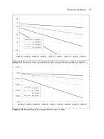
The more detailed analysis of the heat capacities of the solid, aliphatic polyoxides
is summarized in the next two figures. Figure 2.56 displays the deviations of the
calculations from the experiment. Although the agreement is close to the accuracy
of the experiment (±3%), some systematic deviation is visible. It is, however, too
little to interpret as long as no compressibility and expansivity data are available for
2 Basics of Thermal Analysis
__________________________________________________________________

130
Fig. 2.56
Fig. 2.57
amorepreciseC
p
to C
v
conversion. Figure 2.57 indicates that the 
1
and 
3
values
are changing continuously with chemical composition. It is thus possible to estimate

1
and 
3
values for intermediate compositions, and to compute heat capacities of
unknown polyoxides or copolymers of different monomers without reference to
measurement. An interesting observation is that the

1
-values are not very dependent
on crystallinity (see also Fig. 2.50 for polyethylene). The values for

3
, in contrast,