Thermal Analysis of Polymeric Materials Part 7 doc
Bạn đang xem bản rút gọn của tài liệu. Xem và tải ngay bản đầy đủ của tài liệu tại đây (755.15 KB, 60 trang )
4 Thermal Analysis Tools
___________________________________________________________________
346
Fig. 4.70
Fig. 4.69
calorimeter material. Checking the precision of several analyses with sample holders
of different masses, it was found, in addition, that matching sample and reference
sample pans gives higher precision than calculating the heat capacity effect of the
different masses.
In Fig. 4.70 the expression for the heat capacity is completed by inserting the top
equations into the equation for
T of Fig. 4.69. The basic DSC equations contain the
4.3 Differential Scanning Calorimetry
___________________________________________________________________
347
Fig. 4.71
assumptions that the change of reference temperature with time is in steady state, i.e.,
dT
r
/dt = q. Introducing the slope of the recordedbaseline,dT/dT
r
, one obtains a final
equation thatcontains onlyparameters easilyobtained, andfurthermore, can be solved
for the heat capacity of the sample as shown.
The correction term of the basic DSC equation has two factors. The factor in the
first set of parentheses represents close to the overall sample and sample holder (pan)
heat capacity, C
s
. The factor in the second set of parentheses contains a correction
accounting for the different heating rates of reference and sample. For steady-state
(and constant heat capacity), a horizontal baseline is expected with d
T/dT
r
=0;the
heat capacity of the sample is then simply represented by the first term. If, however,
T is not constant, there must be a correction. Fortunately this correction is often
small. Assuming the recording of
T is done with 100 times the sensitivity of T
r
,as
is typical, then, for a
T recording at a 45° angle the correction would be 1% of the
overall sample and holder heat capacity. This error becomes significant if the sample
heat capacity is less than 25% of the heat capacity of sample and holder. Naturally,
it is easy to include the correction in the computer software. The online correction
Tzero™, which is described in more detail in Appendix 11 accounts for this correction
by separately measuring
TandT
b
=T
b
T
r
. Similarly, the heat-flow rates
measured in the DSC of Fig. 4.57 should automatically make this correction.
The second important measurement with a DSC is the determination of heats of
transition. One uses the baseline method for this task. Of special interest is that
during such transitions, steady state is lost. The sample undergoing the transition
remains at the transition temperature by absorbing or evolving the heat of transition
(latent heat). Figure 4.71 represents a typical DSC trace generated during melting.
The temperature difference,
T, is recorded as a function of time or reference
temperature. The melting starts at time t
i
and is completed at time t
f
. During this time
4 Thermal Analysis Tools
___________________________________________________________________
348
Fig. 4.72
span, the reference temperature increases at rate q, while the sample temperature
remains constant at the melting point. The temperature difference
T, thus, must also
increase linearly with rate q. At the beginning of melting the temperature difference
is
T
i
. At the end of melting, when steady state has again been attained, it is T
f
,
reaching the peak of the DSC curve.
The general integration of C
p
to enthalpy goes over temperature, as shown in the
top equation in Fig. 4.71. The second part of the top equation illustrates the insertion
of the expression for mc
p
from Eq. (3) of Fig. 4.69, changed to the variable time and
partially integrated. The final integration to t
f
is shown in the second equation of
Fig. 4.71. The first term of the equation is K times the vertically shaded area, C,in
the graph. The second term is the horizontally shaded area, B, multiplied by K.
Again, the heat of fusion is not directly proportional to the area under the DSC curve
up to the peak. There is, this time, a substantial third term, C
p
'q(t
f
t
i
), marked with
a“?”. An additional difficulty is that area C is not easy to obtain experimentally. It
represents the heat the sample would have absorbed had it continued heating at the
same steady-state rate as before. For its evaluation one needs the zero of the
T
recording which only is available by calibration for asymmetry (see Fig. 2.29).
Next, one may want to calculate the cross-hatched area, A. The calculation is
carried out in Fig. 4.72. Area A represents the return to steady state and can be
described by using the approach to steady state which was derived in Fig. 4.68. The
result represents the first and the last term of the expression for
H
f
as it was given in
Fig. 4.71. This means that under the conditions of identical
Ti and T
f
, one can
make use of the simple baseline method for the heat of fusion determination: The heat
of fusion,
H
f
, is just the area above the baseline in Fig. 4.71, multiplied with K, the
calibration constant. If the baseline deviates substantially from the horizontal,
corrections must be made which are discussed in Fig. 4.80, below.
4.3 Differential Scanning Calorimetry
___________________________________________________________________
349
4.3.7 Applications
Heat Capacity. To make an actual heat capacity measurement, one must first do a
calibration of the constant K. The procedure has been illustrated in Sect. 2.3.1 with
Fig. 2.30. Three consecutive runs should be made. These allow to calculate the
calibration constant K as given in Eq. (3) of Fig. 2.30:
The three runs must agree within experimental error in their absolute amplitude of the
initial and final isotherms. A deviation signals that the heat-loss characteristics of the
calorimeters have changed. The only solution is then to start over. Such mishap
occurs from time to time even with the greatest of care. Another important precaution
is to keep the temperature-range for calibration sufficiently short to have a linear
baseline, i.e., when halving the temperature range, the baseline change must be half.
A well-kept DSC may permit temperature-ranges as wide as 100 K. The amplitudes,
a, should be taken at intervals of 10 K, leading to a calibration table that agrees with
typical heat capacity steps in data tables. Another hint for good quality DSC
measurements is to adjust sample and calibrant amplitudes to similar levels and to
choose the sample mass sufficiently high to minimize errors. Note, however, that too
high amplitudes lead to instrument lags that may limit precision. This is even more
important for TMDSC where the lag may become so large that the modulation is not
experienced by the whole sample.
Figure 2.46 is an example of a heat capacity measurement of polyethylene. The
data were first extrapolated to full and zero crystallinity, as discussed in Sect. 2.3.6,
to characterize the limiting states of solid polyethylene (orthorhombic crystals and
amorphous). The low-temperature data, below about 130 K, were measured by
adiabatic calorimetry as described in Sect. 4.2. Besides the experimental data, the
computed heat capacities from theAdvanced THermal AnalysisSystem, ATHAS, can
also be derived, as shown in Fig. 2.51 and summarized for many polymers in
Appendix 1. This system makes use of an approximate frequency spectrum of the
vibrations in the crystal. At sufficiently low temperature only vibrations contribute
to the heat capacity and missing frequency information can be derived by fitting to the
heat capacity. The skeletal vibrations are vibrations that involve the backbone of the
molecule (torsional and accordion-like motion). Their heat capacity contribution is
most important up to room temperature. The group vibrations are more localized
(C
C and CH stretching and CH bending vibrations) and contribute mainly at
higher temperature. A comparison of the computed and the measured heat capacity
indicates deviations that start at about 250 K and signal other contributions to the heat
capacity. For polyethylene this motion is conformational and of importance to
understand the mechanical properties. Thisexample illustrates the importance ofgood
experimental heat capacity data. Only if C
p
is known, is a sample well characterized.
Besides interpretation of the heat capacity by itself, the heat capacity, C
p,
can also
be used to derive the integral thermodynamic functions, enthalpy, H, entropy, S, and
free enthalpy, G, also called Gibbs function:
4 Thermal Analysis Tools
___________________________________________________________________
350
Fig. 4.73
Polyethylene data are shown in Fig. 2.23. At the equilibrium melting temperature of
416.4 K, the heat of fusion and entropy of fusion are indicated as a step increase. The
free enthalpy shows only a change in slopes, characteristic of a first-order transition.
Actual measurements are available to 600 K. The further data are extrapolated. This
summary allows a close connection between quantitative DSC measurement and the
derivation of thermodynamic data for the limiting phases, as well as a connection to
the molecular motion. In Chaps. 5 to 7 it will be shown that this information is basic
to undertake the final quantitative step, the analysis of nonequilibrium states as are
common in polymeric systems.
Fingerprinting of Materials. Changing toa less quantitative application, materials
are characterized by their phase transition or chemical reactions in what has become
known as fingerprinting. The measurements can be done by DTA with quantitative
information on the transition temperature and made quantitative with respect to the
thermodynamic functions by using DSC. The DSC is furthermore also able to
measure kinetics parameters as shown in Fig. 3.98. The DTA curve of Fig. 4.73, taken
as an unknown, is easily identified as belonging to amyl alcohol (DSC cell A of
Fig. A.9.2, 2
l in air). At least two events are available for identification, the melting
(2) and the boiling (3). It helps the interpretation to look at the sample and know that
it is liquid between (2) and (3) and has evaporated after (3). It is always of importance
to verify transitions observed by DTA by visual inspection. The small exotherm (1)
at about 153 K is due to some crystallization. It occurs on incomplete crystallization
on the initial cooling, a typical behavior of alcohols.
The curve Fig. 4.74 represents a DTA trace, easily identified as belonging to
poly(ethylene terephthalate) which was quenched rapidly from the melt to very low
temperatures before analysis (DTA cell D of Fig. A.9.2, 10 mg of sample in N
2
).
4.3 Differential Scanning Calorimetry
___________________________________________________________________
351
Fig. 4.74
Under such conditions, poly(ethylene terephthalate) remains amorphous on cooling;
i.e., it does not have enough time to crystallize, and thus it freezes to a glass. At point
(1) the increase in heat capacity due to the glass transition can be detected. At point
(2), crystallization occurs with an exotherm. Note that after crystallization the
baseline drops towards the crystalline level. Endotherm (3) indicates the melting, and
finally, there is a broad, exotherm with two peaks (4) due to decomposition. Optical
observation to recognize glass and melt by their clear appearances is helpful.
Microscopy between crossed polarizers is even more definitive for the identification
of an isotropic liquid or glass. More details about this DSC trace will be discussed in
Sect. 5.4.
Figure 4.75 refers to iron analyzed with a high-temperature DTA as sketched H in
Fig. A.9.3. About 30 mg of sample were analyzed in helium. In this case several
solid–solid transitions can be used for the characterization of the sample in addition
to the fusion which is represented by endotherm four. As a group, these solid-solid
transitions are characteristic of iron and can be usable for its identification. A more
quantitative analysis may also allow to distinguish between the many variations of
commercial irons.
The diagram in Fig. 4.76 is a DTA curve of barium chloride with two molecules
of crystal water measured by high-temperature DTA (10 mg sample, in air). The
crystal water is lost in two stages. Identification of these transitions is best through
the weight loss and analysis of the chemical nature of the evolved molecules.
Endotherm (3) is a solid-state transition. Either X-ray diffraction or polarizing
microscopy can characterize it. Finally, anhydrous barium chloride melts at (4),
proven by a loss of the particle character on opening the sample pan after cooling.
Figure 4.77 shows two qualitative DTA traces which can be used to interpret a
chemical reaction between the two compounds. The chemical reaction can be
4 Thermal Analysis Tools
___________________________________________________________________
352
Fig. 4.76
Fig. 4.75
performed either to identify the starting materials or to study the reaction between the
substances. The top curve is a DTA trace of pure acetone (DSC type A of Fig. A.9.2,
1
5 mg of sample, static nitrogen). A simple boiling point is visible. The bottom
trace is of pure p-nitrophenylhydrazine with a melting point, followed by an
exothermic decomposition. The top of Fig. 4.78 is the DTA curve after mixing of both
components in the sample cell. The chemical reaction leading to the product is:
4.3 Differential Scanning Calorimetry
___________________________________________________________________
353
Fig. 4.78
Fig. 4.77
CH
3
HCH
3
H
\| \|
C=O + H
2
N
NphenyleneNO
2
C=NNphenyleneNO
2
+H
2
O
//
CH
3
CH
3
acetone + p-nitrophenylhydrazine
p-nitrophenylhydrazone + water
4 Thermal Analysis Tools
___________________________________________________________________
354
Fig. 4.79
The p-nitrophenylhydrazone has a different thermal behavior. It does not decompose
in the range of temperature used for analysis and does not show the low boiling point
of acetone. To date, little use has been made of this powerful DTA technique in
organic chemical analyses and syntheses.
In Fig. 4.79 the DTA curves for the pyrosynthesis of barium zincate out of barium
carbonate and zinc oxide are shown. The experiment was done by simultaneous DTA
and thermogravimetry on 0.1 cm
3
samples in an oxygen atmosphere. Curve A is the
heating trace of the mixture of barium carbonate and zinc oxide. The DTA curve is
rather complicated because of the BaCO
3
solid–solid transitions. The loss of CO
2
has
already started at 1190 K. The main loss is seen between 1350 and 1500 K. On
cooling after heating to 1750 K, however, a single crystallization peak occurs at
1340 K (curve B). On reheating the mixture, which is shown as curve C, the new
material can be identified as barium zincate by its 1423 K melting temperature.
Unfortunately no explanation is given for the two small peaks at 1450 and 1575 K in
the original research.
Quantitative Analysis of the Glass Transition. Cooling through the glass
transition changes a liquid to a glassy solid. The transition occurs whenever
crystallization is not possible under the given conditions. It is a much more subtle
transition than crystallization, melting, evaporation or chemical reaction in that it has
no enthalpy or entropy of transition. Only its heat capacity changes, as shown in
Fig. 2.117. Characterization of the glass transition requires DSC data of high quality.
At the glass transition, large-amplitude motion becomes possible on heating
(devitrification), and freezes on cooling (vitrification). In contrast to the small-
amplitude vibrational motion in solids,the large-amplitude motion involvestranslation
and rotation, and for polymers, internal rotation (conformational motion). For more
details on the glass transition, see also Chaps. 2 and 5
7. For characterization, one
4.3 Differential Scanning Calorimetry
___________________________________________________________________
355
finds first the glass-transition temperature, T
g
, defined as the temperature of half-
vitrification or devitrification. For homopolymers and other pure materials, the
breadth of the transition, given by T
2
T
1
, and is typically 35 K. For polymers,
blends, and semicrystalline polymers this breadth can increase to more than 100 K.
The beginning, at T
b
, and the end of the transition, at T
e
, are also characteristically
different from sample to sample. All five temperatures of Fig. 2.117 should thus be
recorded together with the change in heat capacity,
C
p
,atT
g
. Since the change into
and out-of the glassy state follows a special, cooperative kinetics, the time-scale in
terms of the heating or cooling rate needs to be recorded also (see Sects. 2.5.6 and
4.4.6).
A sample cooled more slowly vitrifies at lower temperature and stores in this way
information on its thermal history. Reheating the sample gives rise to enthalpy
relaxation or hysteresis as is described in Sect. 6.3. Only when cooling and heating
rates are about equal is there only little hysteresis. Quantitative analysis of the
intrinsic properties of a material and its thermal history is thus possible. Finally, it is
remarked in Fig. 2.117 that it is possible to estimate from
C
p
how many units of the
material analyzed become mobile at T
g
. The DSC of the glass transition is thus a
major source for characterization of materials.
Quantitative Analysis of the Heat of Fusion. The melting transition with its
various characteristic temperatures and the enthalpy of fusion is discussed in Fig. 4.62
as a calibration standard for DSC. In Fig. 4.80 the case is treated where the simple
baseline method of Fig. 4.71–72 is not applicable because of a broad melting range
and a large shift in the baseline. In this case, the baseline must be apportioned
properly to the already absorbed heat of fusion. This change in the baseline can be
estimated by eye, as marked in the figure. The points marked 1/4, 1/2, 3/4, and the
completion of melting are connected as the corrected baseline, if needed with a small
correction for the time needed to reach steady state (lagcorrection). More quantitative
is to use a computer program involving correction of the peak for lags (desmearing to
the true progress of melting [26]) and quantitative deconvolution of the peak as
indicated in the figure by Eq. (2) [27]. The recorded heat capacity that follows the
peak is called the apparent heat capacity, C
p
#
. It is made up of parts of the crystal heat
capacity, amorphous heat capacity, and the latent heat of fusion. In the case of
polymers, the crystallinity is not 100% at low temperature, the samples are semi-
crystalline (see Chap. 5). The total measured heat of fusion is then also only a fraction
of the expected equilibrium value.
Without measuring the heat capacity of the crystalline or semicrystalline sample,
the change of crystallinity can be extracted by solving Eq. (3) [28]. The change of the
heat of fusion with temperature needed for the solution is given in Eq. (1) and is
available from the ATHAS Data Bank as summarized in Appendix 1. The needed
quantity C
p
#
C
p
a
, represents the difference between the measured curve and C
p
a
available from the DSC trace. Figure 4.81 illustrates the change in crystallinity of a
complex block copolymer with two crystallizing species which is discussed in more
detail in Sect. 7.3.3. At low temperature the sample which is phase-separated into a
lamellar structure of the two components consists of glassy and crystalline phases in
each lamella. Next, the oligoether goes through its glass transition without change in
crystallinity. This is followed by the melting of the oligoether crystals, seen by the
4 Thermal Analysis Tools
___________________________________________________________________
356
Fig. 4.81
Fig. 4.80
decrease in oligoether crystallinity to zero. Next is the oligoamide glass transition,
again without change in crystallinity, followed by melting of the oligoamide crystals,
leading to the two-phase structure consisting of the melts of the two components. A
total of six different phases, present in five different phase assemblies have in this
experiment been analyzed quantitatively. The glass transitions are clearly visible in
the heat-capacity traces of Sect. 7.3.3.
4.3 Differential Scanning Calorimetry
___________________________________________________________________
357
Fig. 4.82
Fig. 4.83
A final point to be made is the calibration of the onset temperature of melting with
heating and cooling rates shown in Fig. 4.82. The instrument-lag for the power-
compensated DSC of Fig. 4.58 changes by about 3.5 K on changing q by 100 K min
1
.
On cooling, the In supercools by about 1 K. This can be avoided by calibrating with
transitions that do not supercool, such as isotropizations of liquid crystals or by
seeding using TMDSC (see Sect. 4.4.7). Figure 4.83 shows a similar experiment on
4 Thermal Analysis Tools
___________________________________________________________________
358
Fig. 4.84
a heat-flux DSC as shown in the sketch A of Fig. A.9.2, using different purge gases.
The magnitude of change in the onset temperature of melting is similar to Fig. 4.82.
The rounding in the vicinity of heating rate zero is a specific instrument effect and
does not occur with the operating system of the power-compensated DSC in Fig. 4.82.
When controlling the furnace temperature as in the heat-flux DSC of Fig. 4.57, there
is a mass dependence of the onset of melting as illustrated in Fig. 4.84.
Note, thatsomeDSCs havea lag correction incorporated in theiranalysis software.
Such corrections are, however, only approximations because of the changes with
sample mass, heat conductivity, and environment as is pointed out on pg. 340, above.
More applications of the DSC to the analysis of materials are presented in Sect. 4.4
as well as in Chaps. 6 and 7, below.
4.4 Temperature-modulated Calorimetry
A major advance in differential scanning calorimetry is the application of temperature
modulation, the topic of this section. The principle of measurement with temperature
modulation is not new, the differential scanning technique, TMDSC, however, is.
This technique involves the deconvolution of the heat-flow rate into one part that
follows modulation, the reversing part, and one, that does not, the nonreversing part.
The term reversing is used to distinguish the raw TMDSC data from data proven to be
thermodynamically reversible. Reversing may mean the modulation amplitude
bridges the temperature region of irreversibility or the modulation causes nonlinear or
nonstationary effects, as will be discussed in Sects. 4.4.3 and 4. The first report about
TMDSC was given in 1992 at the 10
th
Meeting of ICTAC [1,22], see also Fig. 2.5.
4.4 Temperature-modulated Calorimetry
___________________________________________________________________
359
Fig. 4.85
4.4.1 Principles of Temperature-modulated DSC
In principle, any DSC can be modulated. As the details of construction of the DSC
equipment vary, it may be advantageous to modulate in different fashions. One can
modulate the block, reference, or sample temperatures, as well as the temperature
difference (proportional to the heat-flow rate). For example, the temperature
modulation of the Mettler-Toledo ADSC™ is controlled by the block-temperature
thermocouple (see Fig. 4.57), while the modulation of the MDSC™ of TA Instruments
in Fig. 4.85 is controlled by the sample thermocouple. Of special interest, perhaps,
would be a modulated dual cell as shown in Fig. 4.56.
In thefollowing discussion, mostcalculations arepatterned after the heatflux DSC
as developed by TA Instruments. The actual software, however, is proprietary and
may use a different route to the same results and also may change as improvements
are made. Similarly, for other instruments the derived equations must be adjusted to
the calorimeter used. A method to combine standard DSC and sawtooth modulation
allows the simultaneous analysis of the standard DSC on linear heating and cooling
segments and the averaged total response, and the evaluation of the reversing heat-
flow rates from the Fourier harmonics of the sawtooth. Details about this versatile
modulation are shown in Appendix 13, which also contains a detailed discussion of
sawtooth modulation linked to the following description of TMDSC.
The major discussion will be based on the DSC shown in Fig. 4.85 which is a
further development of the DSC A of Fig. A.9.2, i.e., TMDSC is an added choice of
operation, not a new instrument. It will be advantageous to do some sample
characterizations in the DSC mode, others in the TMDSC mode. It was noted in
Sect. 4.3 that DSC could be used as a calorimeter or as DTA, similarly TMDSC can
4 Thermal Analysis Tools
___________________________________________________________________
360
Fig. 4.86
be used as a precise, but often slow analysis tool with an average heating or cooling
rate, <q>, of 0
1.0 K min
1
or as DSC with faster rates, typically 550 K min
1
.
Recording only temperature and qualitative heat flows, reduces the DSC to DTA.
Most applicationsof Sect. 4.3 are best done by DTA and DSC(qualitative applications
such as finger printing and quantitative determinations of heat capacity, heats of
reaction and transition) while some of the latter are improved by TMDSC, additional
measurements only are possible with TMDSC as described in Sects. 4.4.6
8.
A basic temperature-modulation equation for the block temperature T
b
is written
in Fig. 4.85, with T
o
representing the isotherm at the beginning of the scanning. The
modulation frequency
7 is equal to 2%/p in units of rad s
1
(1 rad s
1
= 0.1592 Hz) and
p represents the length of one cycle in s. For the present, the block-temperature
modulation is chosen as the reference, i.e., it has been given the phase difference of
zero. The modulation adds, thus, a sinusoidal component to the linear heating ramp
<q>t, where the angular brackets < > indicate the average over the full modulation
cycle. If there is a need to distinguish the instantaneous heating rate from <q>, one
writes the former as q(t). The modulated temperatures drawn in Fig. 4.85 are written
for the quasi-isothermal mode of TMDSC, an experiment where <q> = 0. The
different maximum amplitudes A
T
b
,A
T
r
, and A
T
s
are used to normalize the ordinate in
the graph, so that the phase differences
1 and J can be seen easily. The bottom
equation in Fig. 4.85 is needed to represent the modulated temperature in the presence
of an underlying heating rate <q>
g 0. Figure 4.55 in Sect. 4.3 shows the temperature
changes with time in standard DSC and in TMDSC with a sinusoidal modulation and
an underlying heating rate <q>.
To illustrate the multitudes of possible modulations, the top row of Fig. 4.86
illustrates five segments that can be linked and repeated for modulation of the
temperature. Examples of quasi-isothermal sinusoidal and step-wise modulations are
4.4 Temperature-modulated Calorimetry
___________________________________________________________________
361
Fig. 4.88
Fig. 4.87
shown at the bottom of Fig. 4.86. The sawtooth and two more complex temperature
modulations are displayed in Fig. 4.87. The possible TMDSC modes that result from
sinusoidal modulation are summarized in Fig. 4.88. For the analyses the curves are
often represented by Fourier series. Their basic mathematics is reviewed in
Appendix 13. Each of the various harmonics of a Fourier series of non-sinusoidal
4 Thermal Analysis Tools
___________________________________________________________________
362
Fig. 4.89
modulation can be treated similar to the here discussed sinusoidal modulation, so that
a single sawtooth, for example, can generate multiple-frequency experiments.
Figure 4.89 illustrates the complex sawtoothof Fig. 4.87which can be used to perform
multi-frequency TMDSC with a standard DSC which is programmable for repeat
segments of 14 steps [29]. Each of the five major harmonics possesses a similar
modulation amplitude and the sum of these five harmonics involves most of the
programmed temperature modulation, so that use is made of almost all of the
temperature input to generate the heat-flow-rate response.
4.4.2 Mathematical Treatment
Next, a mathematical description of T
s
is given for a quasi-isothermal run. This type
of run does not only simplify the mathematics, it also is a valuable mode of measuring
C
p
as described in Sect. 4.4.5. In addition, standard TMDSC with <q> g 0 is linked
to the same analysis by a pseudo-isothermal data treatment as described in Sect. 4.4.3.
Figure 4.90 summarizes the separation of the modulated sample temperature into
two components, one is in-phase with T
b
, the other, 90° out-of-phase, i.e., the in-phase
component is described by a sine function, the out-of-phase curve by a cosine
function. The figure also shows the description of the time-dependent T
s
as the sum
of the two components. The sketch of the unit circle links the maximum amplitudes
of the two components. Furthermore, the standard addition theorem of trigonometric
functions in the box at the bottom expresses that T
s
is a phase-shifted sine curve.
The additional boxed equation on the right side of Fig. 4.90 introduces a
convenient description of the temperature using a complex notation. The trigonomet-
ric functions can be written as sin
=(i/2)(e
i
e
i
)andcos = (1/2)(e
i
+e
i
)
where i =
1
,sothatsin +icos =ie
i
. The real part of the shown equation
4.4 Temperature-modulated Calorimetry
___________________________________________________________________
363
Fig. 4.90
represents then T
s
. The chosen non-standard format of the complex number is
necessary since at time zero T
s
=T
r
=T
b
=T
o
and T = 0. A phase-shift by %/2 leads
to the standard notation of complex numbers, given in Sect. 2.3.5 as Eqs. (1).
Naturally all these equations apply only to the steady state, illustrated by the right
graph of Fig. 4.55. Its derivation is similar to the discussion for steady state in a
standard DSC given in Fig. 4.68. One solves the differential equation for heat-flow
rate, as in Fig. 4.67, but including also the term describing the modulation of T
s
:
The solution of this differential equation can be found in any handbook and checked
by carrying out the differentiation suggested. The terms in the first brackets of the
solution are as found for the standard DSC in Fig. 4.68, the second bracket describes
the settling of the modulation to steady state:
At sufficiently long time, steady state is reached (Kt >> C
p
) and the equation reduces
after division by C
p
to the steady state temperature T(t) T
o
. It will then be applied
in all further discussions, unless stated otherwise:
4 Thermal Analysis Tools
___________________________________________________________________
364
Fig. 4.91
The next step is the analysis of a single, sinusoidal modulation in the DSC
environment. In the top line of Fig. 4.91 Eq. (2) of Fig. 4.69 is repeated, the equation
for the measurement of heat capacity in a standard DSC. The second line shows the
needed insertions for T
s
and T for the case of modulation. When referred to T
b
,the
phase difference of
T is equal to and its real part is the cosine, the derivative of the
sine, as given by the top equation. Next, the insertion and simplification of the
resulting equation are shown. By equating the real and imaginary parts of the
equations separately, one finds the equations listed at the bottom of Fig. 4.91. These
equations suggest immediately the boxed expression for C
s
C
r
in Fig. 4.92.
Several types of measurement can be made. First, one can use, as before, an empty
pan as reference of a weight identical to the sample pan. The bottom equation of
Fig. 4.92 suggests that in this case the sample heat capacity is just the ratio of the
modulation amplitudes of
TandT
s
multiplied with a calibration factor that is
dependent on thefrequency and the mass of the empty pans. Standardizing on a single
pan weight (such as 22 mg) and frequency (such as 60 s) permits measurements of the
reversing heat capacity with a method that is not more difficult than for the standard
DSC, seen in Figs. 2.28–30. Another simplifying experimental set-up is to use no
reference pan at all. Figure 4.92 shows that in this case the pan-weight dependence
4.4 Temperature-modulated Calorimetry
___________________________________________________________________
365
Fig. 4.92
of the calibration disappears. As a disadvantage, the measured quantity is, however,
not the sample heat capacity directly, as before, but the measurement is the heat
capacity of sample plus sample-pan.
More specific information was derived for the Mettler-Toledo DSC, as described
in Figure 4.57 [30]. For the calculations, the DSC was modeled with an analog
electrical circuit of the type shown in Appendix 11 for the elimination of asymmetry
and pan effects. The Mettler-ToledoDSC is also of the heat-flux type, but the control-
thermocouple is located close to the heater. The model considered the thermal
resistances between heater and
T-sensor, R, sensor and sample, R
s
, and a possible
cross-flow between sample and reference, R' [30]. Equations (1) and (2) in Fig. 4.93
show the equations which can be derived for the heat capacity, C
s
m
, and the phase
angle
. A series of quasi-isothermal measurements for different masses, m, and
frequencies,
7 are shown in Fig. 4.93 for a sawtooth modulation. Uncorrected data
for
and 7 are given by the open symbols. They were calculated using the bottom-
right equation in Fig. 4.92. For the short periods with p less than 100 s, strong
deviations occur. The known specific heat capacity of thealuminumsample is marked
by the dotted, horizontal line. The constant, negative offset at long periods, p, was
corrected by the usual calibration with sapphire (Al
2
O
3
) with a constant shift over the
whole frequency range. A value of 35.38 mW K
1
was found for K* at 298 K. The
deviations at small p were then interpreted with Eq. (1) making the assumption that
they originate from the coupling between the various thermal resistance parameters.
To determine
, Eq. (2) was fitted with the true specific heat capacity of the
aluminum. The results of the fitting are indicated in Fig. 4.93 by the dashed lines.
The value of R
s
+R
2
/(2R + R') of Eq. (2) has a sample-mass independent value of
1.34/K*. Finally, the corrected values for the specific heat capacities were calculated
with Eq. (1) and marked in Fig. 4.93 by the filled symbols. All frequency and mass
4 Thermal Analysis Tools
___________________________________________________________________
366
Fig. 4.93
dependence could be removed by this calculation. The RMS error of the data is
0.77%. Although measurements could now be made down to periods of about 20 s,
the data evaluation is still cumbersome and not all thermal resistances one would
expect to affect the data could be evaluated, such as the resistances within the sample
pan and the heat supplied by the purge gas. If these latter effects cause significant
changes or delays in the modulation, the parameters in the just discussed equations in
Fig. 4.93 are just fitting parameters.
To find a universal equation which can be used to calibrate the data for different
masses, frequencies, sample packing, and purge-gas configuration, the power-
compensated DSC was employed [31]. Its operation is described in Figs. 4.58–61.
Equation (1) in Fig. 4.94 repeats the approximate heat capacity determination from
standard DSC using the total (averaged) heat-flow rate and rate of change of sample
temperature (see Fig. 4.76, <HF> = K
T, C
s
C
r
=mc
p
, <q> = q). Equation (2)
progresses to the quasi-isothermal, reversing heat capacity given in Fig. 4.92 at the
bottom left. Finally, Eq. (3) shows the substitution of an empirical parameter,
-, into
the square root of the equation in Fig. 4.92 which can be calibrated. For very low
frequencies,
- approaches C
r
/K, as expected from Fig. 4.92. This equation was
introduced already in Fig. 4.54 as basic equation for the data evaluation.
The experiments on the left of Fig. 4.94 show the results for quasi-isothermal,
sawtooth-modulated polystyrene as a function of period and amplitude (12 mg, at
298.15 K) [31]. The filled symbols were calculated using Eq. (1). Data were chosen
when steady state was most closely approached, i.e., at the time just before switching
the direction of temperature change or over the range of time of obvious steady state.
The thin solid line is the expected heat capacity, the dotted lines mark a ±1% error
range. The bold line is an arbitrary fit to the open symbols. The different modulation
amplitudes were realized by choosing different heating and cooling rates. The
4.4 Temperature-modulated Calorimetry
___________________________________________________________________
367
Fig. 4.94
modulation amplitude seems to have no influence on the dependence on period. The
open symbols represent the reversing specific heat capacity. They were calculated
using the amplitudes of the first harmonic of the Fourier fit of heat-flow rate and
sample temperature to Eq. (2). In the case of the Fourier fit, the deviation from the
true heat capacity starts at a period of
96 s. In the case of standard DSC, this critical
value is shifted to
48 s. The influence of the sample mass was analyzed for Al. The
data are shown on the right in Fig. 4.94. An increasing sample mass, as well as a
shorter modulation period reduces the measured heat capacity. Again, the Fourier fit
results in larger deviations from the expected value when compared to the heat
capacity calculated by the standard DSC equation, Eq. (1).
Figure 4.95 illustrates the evaluation of the constant
- as the slope of a plot of the
square of the reciprocal of the uncorrected specific heat capacity as a function of the
square of the frequency as suggested by Eqs. (2) and (3) of Fig. 4.94. Note that the
calibration run of the sapphire and the polystyrene have different values of
In
addition, the asymmetry of the calorimeter must be corrected in a similar process as
discussed in Sect. 4.4.4, again with a different value of
Online elimination of the
effects of asymmetry and different pan mass, as described in Appendix 11, should
improve the ease of measurement. This method of analysis increases the precision of
the reversing data gained at high frequency, and also the overall precision, since a
larger number of measurements are made during the establishment of
- as a function
of frequency and spurious effects not following the modulation are eliminated.
A simplification of the multi-frequency measurements can be done by using not
only the first harmonic of sawtooth modulation for the calculation of the heat capacity,
but using several, as shown in Fig. 4.96 [32]. A single run can in this way complete
many data points. As in Fig. 4.95, the lower frequencies have a constant
-, while at
4 Thermal Analysis Tools
___________________________________________________________________
368
Fig. 4.95
Fig. 4.96
higher frequency,
- varies. Since the change of - with frequency is a continuous
curve, rather high-frequency data should be usable for measurement. Since the higher
harmonics in the sawtooth response have a lower amplitude, the complex sawtooth of
Fig. 4.89 was developed with five harmonics of similar amplitudes [29]. A
comparison of this type of measurement was made with all three instruments featured
in this section in Figs. 4.57, 4.58, and 4.85 [33–35]. All data could be represented
4.4 Temperature-modulated Calorimetry
___________________________________________________________________
369
Fig. 4.97
with empirically found values of
- and precision as high as ±0.1% was approached,
matching the typical precision of adiabatic calorimetry (see Sect. 4.2).
4.4.3 Data Treatment and Modeling
The data treatment of TMDSC is summarized in Figs. 4.97 and 4.98. It uses the
instantaneous values of
T(t), represented by curve A in Fig. 4.99 and involves their
sliding averages (< >) over full modulation periods, p, as given by curve B.By
subtracting this average from
T(t), based on curve C,apseudo-isothermal analysis
becomes possible. The averages containnone ofthe sinusoidal modulation effectsand
are called the total heat-flow rate (<HF(t)> or <
0(t)>, being proportional to <T(t)>).
This analysis is strictly valid only, if there is a linear response of the DSC, i.e.,
doubling any of the variables in Fig. 4.54 (m, q, and c
p
, and also any latent-heat)
doubles the response,
T. In addition, the total quantity, B,mustbestationary, i.e.,
change linearly or be constant over the whole period analyzed. The expression for the
sample temperature, T
s
(t), is calculated analogously and should agree with the
parameter set for the run, so that <T
s
(t)> is the total temperature calculated from the
chosen underlying heating rate (= T(0) + <q> t). These averages make use of data
measured over a time range ±p/2, i.e., the output of TMDSC can only be displayed
with a delay from t
o
, the time of measurement of the calculated value.
Part 2 in Fig. 4.97 aims at finding the amplitude of curve C, the peudo-isothermal
response, <A
(t)>, called the reversing heat-flow rate. Again, <A
T
s
(t)> is set as a run
parameter and needs only a check that, indeed, it is reached. The amplitude <A
(t)>
is the first harmonic of the Fourier series for
T(t). The first step is the finding of D
and E, where the capital letters indicate the corresponding curves in Figs. 4.99 to
4.102. Note: D =<A
>sin(7t )sin7tandE =<A
>sin(7t )cos7t. The
4 Thermal Analysis Tools
___________________________________________________________________
370
Fig. 4.99
Fig. 4.98
value of <A
> is then found from renewed averaging over one period, i.e., one forms
<
T(t
2
)
sin
>=(A
/2) cos =<D>=F, and <T(t
2
)
cos
>=(A
/2) sin =<E>=G,as
shown in Fig. 4.98 and displayed in Fig. 4.99. The amplitude <A
(t
2
)> = H is
obtained from the sums of the squares of F and G. To further improve H, smoothing
is done by one more averaging, as shown in the box of Fig. 4.98. This yields the final
output I. The data used for I cover two modulation periods and are displayed at t
3
,1.5