Vision Systems - Applications Part 6 pdf

3D Cameras: 3D Computer Vision of wide Scope
191
adjusted for all pixel elements together, one might guess that it is the best strategy to avoid
each pixel from oversaturation. Focusing the small object will most likely decrease the
accuracy for the remaining scene. This also means, that the signal level for objects with low
diffuse reflectivity will be low if objects with high reflectivity are in the same range of vision
during measurement.
One suitable method is to merge multiple captures at different integration times. It reduces
the frame rate but increases the dynamic range.
In [May, 2006] we have presented an alternative integration time controller based on mean
intensity measurements. This solution was empirically found and showed a suitable
dynamic range for our experiments without affecting the frame rate. It also alleviates the
effects of small bothering areas. The averaged amplitude in dependency of intensity can be
seen in figure 8.
Figure 8. Relation between mean amplitude and mean intensity. Note that the characteristic
is now a mixture of the characteristic of each single pixel (cf. figure 6)
We used a proportional closed-loop controller to adjust the integration time from one frame
to the next as shown in the following itemization.
The control deviation variable I
a
was assigned with a value of 15000 for the illustrations in
this chapter. It has been chosen conservatively with respect to the characteristic shown in
figure 8.
1. Calculate the mean intensity
t
I from the intensity dataset I
t
at time t.
2. Determine control deviation
att
IID −= .

3. Update control variable
ttpt
cDVc +⋅−=
+1
for grabbing the next frame, where c
t
and c
t+1
are the integration times for two frames following one another, V
p
the proportional
closed loop deviation parameter and
c
0
a suitable initial value.
Independent of the chosen control method, the integration time has always to be adjusted
with respect to the application. A change of integration time causes an apparent motion
considering the distance measurement values. Therefore, it is necessary for the application
to take the presence of control deviation into account while using an automatic integration
time controller.
Vision Systems: Applications
192
The newest model from Mesa Imaging, the SwissRanger SR-3000 provides an automatic
integration time exposure based on the amplitude values. For most scenes it works properly.
In some cases of fast scene change it could occur that a proper integration time cannot be
found. This is up to the missing intensity information due to the backlight suppression on
chip. The amplitude diagram does not provide a non-ambiguous working point. A short
discussion on the backlight suppression will be given in section 3.3.
3.2.2 Consideration of accuracy
It is not possible to guarantee certain accuracies for measurements of unknown scenes, since

they are affected by the influences mentioned above. However, the possibility to evolve the
accuracy information for each pixel eases that circumstance. In section 4 two examples using
this information will be explained. For determining the accuracy equation (7) is used.
Assuming that the parameters of the camera (in general this is the integration time for users)
are optimally adjusted, the accuracy only depends on the object’s distance and its
reflectivity. For indoor applications with less background illumination, the accuracy is
linearly decreasing (see equation (8)). Applying a simple threshold is one option for filtering
out inaccurate parts of an image. Setting a suitable threshold primarily depends on the
application. Lange stated with respect to the dependency between accuracy and distance
[Lange, 2000]: “This is an important fact for navigation applications, where a high accuracy
is often only needed close to the target“. This statement does not hold for every other
application like mapping, where unambiguousness is essential for registration.
Unambiguous tokens are often distributed over the entire scene. Higher distances between
these tokens provide geometrically higher accuracies for the alignment of two scans. After
this consideration, increasing the threshold linearly with the distance for indoor applications
suggests itself. This approach enlarges the information gain from the background and can
be seen in figure 9.
A light source in the scene decreases the reachable accuracy. The influence of the accuracy
threshold can be seen in figure 10. Bothered areas are reliably removed. The figure shows
also that the small bothering area of the lamp does not much influence the integration time
controller based on mean intensity values, even so that the surrounding area is determined
precisely.

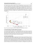
Figure 9. Two images taken with a SwissRanger SR-2 device of the same scene. Left image:
without filtering. Right image: with accuracy filter. Only data points with an accuracy better
than 50mm are remaining
3D Cameras: 3D Computer Vision of wide Scope
193

Figure 10. Influence of light emitting sources. Top row: The light source is switched off.
Lower Row: The light source is switched on. Note that the bothered area could reliably be
detected
3.3. Latest Improvements and expected Innovations in Future
Considering equation (7) a large background illumination (I
b
>> I
l
) highly affects the
sensor’s accuracy by increasing the shot noise and lowering its dynamics. Some sensors
nowadays are equipped with some background light suppression functionalities, e.g.
spectral filters or circuits for constant component suppression, which are increasing the
signal-to-noise ratio [Moeller et al., 2005], [Buettgen et al., 2006].
Suppressing the background signal has one drawback. The amplitude represents the
infrared reflectivity and not the reflectivity we sense as human-beings. This might take
effects on computer vision systems inspired by our human visual sense, e.g. [Frintrop, 2006].
Some works in the past had also proposed a circuit structure for a pixel-wise-integration
capability [Schneider, 2003], [Lehmann, 2004]. Unfortunately, this technology did not
become widely accepted due to a lower fill-factor. Lange explained the importance of the
optical fill factor as follows [Lange, 2000]: “The optical power of the modulated illumination
source is both expensive and limited by eye-safety regulations. This requires the best
possible optical fill factor for an efficient use of the optical power and hence a high
measurement resolution.”
4. 3D Vision Applications
This section investigates the practical influence of upper mentioned thoughts by presenting
some typical applications in the domain of autonomous robotics currently investigated by
us. Since 3D cameras are comparatively new to other 3D sensors like laser scanners or stereo
cameras, the porting of algorithms defines a novelty per se; e.g. one of the first 3D maps
Vision Systems: Applications
194

created with registration approaches mostly applied to laser scanner systems up to now was
presented at the IEEE/RSJ International Conference on Intelligent Robots and Systems in
2006 [Ohno, 2006]. The difficulties to come across with these sensors are discussed in this
section. Furthermore, a first examination on the capabilities for tackling environment
dynamics will follow.
4.1. Registration of 3D Measurements
One suitable registration method for range data sets is called the Iterative Closest Points
(ICP) algorithm and was introduced by Besl and McKay in 1992 [Besl & McKay, 1992]. For
the readers convenience a brief description of this algorithm is repeated in this section.
Given two independently acquired sets of 3D points,
M (model set) and D (data set), which
correspond to a single shape, we aim to find the transformation consisting of a rotation
R
and a translation t which minimizes the following cost function:
.)(),(
1
2
,
¦¦
==
+−=
M
i
ji
D
ij
ji
tRdmtRE
ω
(9)

ǚ
i,j
is assigned 1 if the i-th point of M describes the same point in space as the j-th point of D.
Otherwise ǚ
i,j
is 0. Two things have to be calculated: First, the corresponding points, and
second, the transformation (R,t) that minimizes E(R,t) on the base of the corresponding
points. The ICP algorithm calculates iteratively the point correspondences. In each iteration
step, the algorithm selects the closest points as correspondences and calculates the
transformation (R,t) for minimizing equation (9). The assumption is that in the last iteration
step the point correspondences are correct. Besl and McKay prove that the method
terminates in a minimum [Besl & McKay, 1992]. However, this theorem does not hold in our
case, since we use a maximum tolerable distance d
max
for associating the scan data. Such a
threshold is required though, given that 3D scans overlap only partially. The distance and
the degree of overlapping have a non-neglective influence of the registration accuracy.
4.2. 3D Mapping – Invading the Domain of Laser Scanners
The ICP approach is one upon the standard registration approaches used for data from 3D
laser scanners. Since the degree of overlapping is important for the registration accuracy, the
huge field of view and the high range of laser scanners are advantages over 3D cameras
(compare table 1 with table 3). The following section describes our mapping experiments
with the SwissRanger SR-2 device.
The image in figure 11 shows a single scan taken with the IAIS 3D laser scanner. The scan
provides a 180 degree field of view. Getting the entire scene into range of vision can be done
by taking only two scans in this example. Nevertheless, a sufficient overlap can be
guaranteed to register both scans. Of course there are some uncovered areas due to
shadowing effects, but that is not the important fact for comparing the quality of
registration. A smaller field of view makes it necessary to take more scans for the coverage
of the same area within the range of vision. The image in figure 12 shows an identical scene

taken with a SwissRanger SR-2 device. There were 18 3D images necessary for a
circumferential view with sufficient overlap. Each 3D image was registered with its
previous 3D image using the ICP approach.
3D Cameras: 3D Computer Vision of wide Scope
195
Figure 11. 3D scan taken with an IAIS 3D laser scanner
Figure 12. 3D map created from multiple SwissRanger SR-2 3D images. The map was
registered with the ICP approach. Note the gap at the bottom of the image, that indicates the
accumulating error
4.2.1. “Closing the Loop”
The registration of 3D image sequences causes a non-neglective accumulation error. This
effect is represented by the large gap at the bottom of the image in figure 12. These effects
have also been investigated in detail for large 3D maps taken with 3D laser scanners, e.g. in
[Surmann et al., 2004], [Cole & Newman, 2006]. For a smaller field of view these effects
occur faster, because of the smaller size of integration steps. Determining the closure of a
loop can be used in these cases to expand the overall error on each 3D image. This implies
that the present captured scene has to be recognized to be already one of the previous
captured scenes.
Vision Systems: Applications
196
4.2.2. “Bridging the Gap“
The second difficulty for the registration approach is that a limited field of view makes it
more unlikely to measure enough unambiguous geometric tokens in the space of distance
data or even sufficient structure in the space of grayscale data (i.e. amplitude or intensity).
This issue is called the aperture problem in computer vision. It occurs for instance for
images taken towards a huge homogeneous wall (see [Spies et al., 2002] for an illustration).
In the image of figure 12 the largest errors occurred for the images taken along the corridor.
Although points with a decreasing accuracy depending on the distance (see section 3.2.2)
were considered, only the small areas at the left and the right border contained some fairly
accurate points, which made it difficult to determine the precise pose. This inaccuracy is

mostly indicated in this figure by the non-parallel arrangement of the corridor walls. The
only feasible solution to this problem is a utilization of different perspectives.
4.3. 3D Object Localization
Object detection is a highly investigated field of research since a very long period of time. A
very challenging task here is to determine the exact pose of the detected objects. Either this
information is just implicitly available since the algorithm is not very stable against object
transformations or the pose information is explicit but not very precise and therefore not
very reliable. For reasoning about the environment it may be enough to know which objects
are present and where they are located but especially for manipulation tasks it is essential to
know the object pose as precise as possible. Examples for such applications are ranging from
“pick and place” tasks of disordered components in industrial applications to handling task
of household articles in service-robotic applications.
In comparison to color camera based systems the use of 3D range sensors for object
localization provide much better results regarding the object pose. For example Nuechter et
al. [Nuechter et al., 2005] presented a system for localizing objects in 3D laser scans. They
used a 3D laser scanner for the detection and localization of objects in office environments.
Depending on the application one drawback of this approach is the time consuming 3D
laser scan which needs at least 3.2 seconds for a single scan (cf. table 1). Using a faster 3D
range sensor would increase the timing performance of such a system essentially and thus
open a much broader field of applications.
Therefore Fraunhofer IAIS is developing an object localization system which uses range data
from a 3D camera. The development of this system is part of the DESIRE research project
which is founded by the German Federal Ministry of Education and Research (BMBF) under
grant no. 01IME01B. It will be integrated into a complex perception system of a mobile
service-robot. In difference to the work of Nuechter et al. the object detection in the DESIRE
perception system is mainly based on information from a stereo vision system since many
objects are providing many distinguishable features in their texture. With the resulting
hypothesis of the object and it’s estimated pose a 3D image of the object is taken and
together with the hypothesis it is used as input for the object localization.
The localization itself is based on an ICP based scan matching algorithm (cf. section 4.1).

Therefore each object is registered in a database with a point cloud model. This model is
used for matching with the real object data. For determining the pose, the model is moved
into the estimated object pose and the ICP algorithm starts to match the object model and
the object data. The real object pose is given by a homogeneous transformation. Using this
3D Cameras: 3D Computer Vision of wide Scope
197
object localization system in real world applications brings some challenges, which are
discussed in the next subsection.
4.3.1 Challenges
The first challenge is the pose ambiguities of many objects. Figure 13 shows a typical object
for a home service-robot application, a box of instant mashed potatoes. The cuboid shape of
the box has three plains of symmetry which results in the ambiguities of the pose.
Considering only the shape of the object, very often the result of the object localization is not
a single pose but a set of possible poses, depending on the number of symmetry planes. For
determining the real pose of an object other information than only range data are required,
for example the texture. Most 3D cameras additionally providing gray scale images which
give information about the texture but with the provided resolution of around 26.000 pixels
and an aperture angle of around 45° the resolution is not sufficient enough for stable texture
identification. Instead, e.g., a color camera system can be used to solve this ambiguity. This
requires a close cooperation between the object localization system and another
classification system which uses color camera images and a calibration between the two
sensor systems. As soon as future 3D cameras are providing higher resolutions and maybe
also color images, object identification and localization can be done by using only data from
a 3D camera.
Figure 13. An instant mashed potatoes box. Because of the symmetry plains of the cuboid
shape the pose determination gives a set of possible poses. Left: Colour image from a digital
camera. Right: 3D range image from the Swissranger SR-2
Another challenge is close related to the properties of 3D cameras and the resulting ability to
provide precise range images of the objects. It was shown that the ICP based scan matching
algorithm is very reliable and precise with data from a 3D laser scanner, which are always

providing a full point cloud of the scanned scene [Nuechter, 2006], [Mueller, 2006]. The
accuracy is static or at least proportional to the distance. As described in section 3.2.2 the
accuracy of 3D camera data is influenced by several factors. One of these factors for example
is the reflectivity of the measured objects. The camera is designed for measuring diffuse
light reflections but many objects are made of a mixture of specular and diffuse reflecting
materials. Figure 14 shows color images from a digital camera and range images from the
Swissrange SR-2 of a tin from different viewpoints. The front view gives reliable range data
of the tin since the cover of the tin is made of paper which gives diffuse reflections. In the
second image the cameras are located a little bit above and the paper cover as well as high
reflecting metal top is visible in the color image. The range image does not show the top
Vision Systems: Applications
198
since the calculated accuracy of these data points is less than 30 mm. This is a loss of
information which highly influences the result of the ICP matching algorithm.
Figure 14. Images of a tin from different view points. Depending on the reflectivity of the
objects material the range data accuracy is different. In the range images all data points with
a calculated accuracy less than 30mm are rejected. Left: The front view gives good 3D data
since the tin cover reflects diffuse. Middle: From a view point above the tin, the cover as
well as the metal top is visible. The high reflectivity of the top results in bad accuracy so that
only the cover part is visible in the range image. Right: From this point of view, only the
high metal top is visible. In the range image only some small parts of the tin are visible
4.4. 3D Feature Tracking
Using 3D cameras to full capacity necessitates taking advantage of their high frame rate.
This enables the consideration of environment dynamics. In this subsection a feature
tracking application is presented to give an example of applications that demand high frame
rates. Most existing approaches are based on 2D grayscale images from 2D cameras since
they were the only affordable sensor type with a high update rate and resolution in the past.
An important assumption for the calculation of features in grayscale images is called
intensity constancy assumption. Changes in intensity are therefore only caused by motion.
The displacement of two images is also called optical flow. An extension to 3D can be found

in [Vedula et al., 1999] and [Spies et al., 2002]. The intensity constancy assumption is being
combined with a depth constancy assumption. The displacement of two images can be
calculated more robustly. This section will not handle scene flow. However the depth value
of features in the amplitude space should be examined so that the following two questions
are answered:
•
Is the resolution and quality of the amplitude images from 3D cameras good enough to
apply feature tracking kernels?
•
How stable is the depth value of features gathered in the amplitude space?
To answer these questions a Kanade-Lucas-Tomasi (KLT) feature tracker is applied [Shi,
1994]. This approach locates features considering the minimum eigenvalue of each 2x2
3D Cameras: 3D Computer Vision of wide Scope
199
gradient matrix. Tracking features frame by frame is done by an extension of previous
Newton-Raphson style search methods. The entire approach also considers multi-resolution
to enlarge possible displacements between the two frames. Figure 15 shows the result of
calculating features in two frames following one another. Features in the present frame (left
feature) are connected with features from the previous frame (right feature) with a thin line.
The images in figure 15 show that many edges in the depth space are associated with edges
in the amplitude space. The experimental standard deviation for that scene was determined
by taking the feature’s mean depth value of 100 images. The standard deviation was then
calculated from 100 images of the same scene. These experiments have been performed two
times, first without a threshold and second with an accuracy threshold of 50mm (cf. formula
7). The results are shown in table 4 and 5.
Experimental standard deviation ǔ = 0.053m, Threshold ƦR = 
Feature # Considered
Mean Dist
[m]
Min Dev

[m]
Max Dev
[m]
1 Yes -2.594 -0.112 0.068
2 Yes -2.686 -0.027 0.028
3 Yes -2.882 -0.029 0.030
4 Yes -2.895
-0.178 0.169
5 Yes -2.731
-0.141 0.158
6 Yes -2.750 -0.037 0.037
7 Yes -2.702
-0.174 0.196
8 Yes -2.855
-0.146 0.119
9 Yes -2.761 -0.018 0.018
10 Yes -2.711 -0.021 0.025
Table 4. Distance values and deviation of the first ten features calculated from the scene
shown in the left image of figure 15 with no threshold applied
Experimental standard deviation ǔ = 0.017m, Threshold ƦR = 50mm
Feature # Considered
Mean Dist
[m]
Min Dev
[m]
Max Dev
[m]
1 Yes -2.592 -0.110 0.056
2 Yes -2.684 -0.017 0.029
3 Yes -2.881 -0.031 0.017

4 No -2.901
-0.158 0.125
5 Yes -2.733
-0.176 0.118
6 Yes -2.751 -0.025 0.030
7 No -2.863
-0.185 0.146
8 No -2.697
-0.169 0.134
9 Yes -2.760 -0.019 0.015
10 Yes -2.711 -0.017 0.020
Table 5. Distance values and deviation of the first ten features calculated from the scene
shown in the left image of figure 15 with a threshold of 50mm
The reason for the high standard deviation is the noise criterion for edges. The signal
reflected by an edge is a mixture of the background and object signal. A description of this
Vision Systems: Applications
200
effect is given in [Gut, 2004]. Applying an accuracy threshold alleviates this effect. The
standard deviation is decreased significantly. This approach has to be balanced with the
number of features found in an image. Applying a more restrictive threshold might decrease
the number of features too much. For the example described in this section an accuracy
threshold of ƦR = 10mm decreases the number of features to 2 and the experimental
standard deviation ǔ to 0.01m.

Figure 15. Left image: Amplitude image showing the tracking of KLT-features from two
frames following one another. Right image: Side view of a 3D point cloud. Note the
appearance of jump edges at the border area
5. Summary and Future work
First of all, a short comparison of range sensors and their underlying principles was given.
The chapter further focused on 3D cameras. The latest innovations have given a significant

improvement for the measurement accuracy, wherefore this technology has attracted
attention in the robotics community. This was also the motivation for the examination in this
chapter. On this account, several applications were presented, which represents common
problems in the domain of autonomous robotics.
For the mapping example of static scenes, some difficulties have been shown. The low
range, low apex angle and low dynamic range compared with 3D laser scanners, raised a lot
of problems. Therefore, laser scanning is still the preferred technology for this use case.
Based on the first experiences with the Swissranger SR-2 and the ICP based object
localization, we will further develop the system and concentrate on the reliability and the
robustness against inaccuracies in the initial pose estimation. Important for the reliability is
knowledge about the accuracy of the determined pose. Indicators for this accuracy are, e.g.,
the number of matched points of the object data or the mean distance between found model-
scene point correspondences.
The feature tracking example highlights the potential for dynamic environments. Use cases
with requirements of dynamic sensing are predestinated for 3D cameras. Whatever, these
are the application areas 3D cameras were once developed.
Our ongoing research in this field will concentrate on dynamic sensing in future. We are
looking forward to new sensor innovations!
3D Cameras: 3D Computer Vision of wide Scope
201
6. References
Besl, P. & McKay, N. (1992). A Method for Registration of 3-D Shapes, IEEE Transactions on
Pattern Analysis and Machine Intelligence, Vol. 14, No. 2, (February 1992) pp. 239-256,
ISSN: 0162-8828
Buettgen, B.; Oggier, T.; Lehmann, M.; Kaufmann, R.; Neukom, S.; Richter, M.; Schweizer,
M.; Beyeler, D.; Cook, R.; Gimkiewicz, C.; Urban, C.; Metzler, P.; Seitz, P.;
Lustenberger, F. (2006). High-speed and high-sensitive demodulation pixel for 3D
imaging, In: Three-Dimensional Image Capture and Applications VII. Proceedings of
SPIE, Vol. 6056, (January 2006) pp. 22-33, DOI: 10.1117/12.642305
Cole, M. D. & Newman P. M. (2006). Using Laser Range Data for 3D SLAM in Outdoor

Environments, In Proceedings of the IEEE International Conference on Robotics and
Automation (ICRA), pp. 1556-1563, Orlando, Florida, USA, May 2006
CSEM SA (2007), SwissRanger SR-3000 - miniature 3D time-of-flight range camera, Retrieved
January 31, 2007, from
Frintrop, S. (2006). A Visual Attention System for Object Detection and Goal-Directed Search,
Springer-Verlag, ISBN: 3540327592, Berlin/Heidelberg
Fraunhofer IAIS (2007). 3D-Laser-Scanner, Fraunhofer Institute for Intelligent Analysis and
Information Systems, Retrieved January 31, 2007, from
Gut, O. (2004). Untersuchungen des 3D-Sensors SwissRanger, Eidgenössische Technische
Hochschule Zürich, Retrieved January 21, 2007, from
/>_fe.html
Hokuyo Automatic (2007), Scanning laser range finder for robotics URG-04LX, Retrieved
January 31, 2007, from
Ibeo Automobile Sensor GmbH (2007), Ibeo ALASCA XT Educational System, Retrieved
January 31, 2007, from
/>Kawata, H.; Ohya, A.; Yuta, S.; Santosh, W. & Mori, T. (2005). Development of ultra-small
lightweight optical range sensor system, International Conference on Intelligent Robots
and Systems 2005, Edmonton, Alberta, Canada, August 2005.
Lange, R. (2000). 3D time-of-flight distance measurement with custom solid-state image
sensors in CMOS/CCD-technology, Dissertation, University of Siegen, 2000
Lehmann, M.; Buettgen, B.; Kaufmann, R.; Oggier, T.; Stamm, M.; Richter, M.; Schweizer,
M.; Metzler, P.; Lustenberger, F.; Blanc, N. (2004). CSEM Scientific & technical Report
2004, CSEM Centre Suisse d’Electronique et de Microtechnique SA, Retrieved
January 20, 2007, from

Lowe, D. G. (2004). Distinctive Image Features from Scale-Invariant Keypoints, International
Journal of Computer Vision, Vol. 60, No. 2, (November 2004) pp. 91-110, ISSN: 0920-
5691
Lucas, B. D. & Kanade, T. (1981). An Interative Image Registration Technique with an
Application to Stereo Vision, In Proceedings of the 7th International Conference on

Artificial Intelligence (IJCAI), pp. 674-679, Vancouver, British Columbia, August 1981
May, S.; Werner, B.; Surmann, H.; Pervoelz, K. (2006). 3D time-of-flight cameras for mobile
robotics, In Proceedings of the IEEE/RSJ International Conference on Intelligent Robots
and Systems (IROS), pp. 790-795, Beijing, China, October 2006
Vision Systems: Applications
202
Moeller, T.; Kraft H.; Frey, J.; Albrecht, M.; Lange, R. (2005). Robust 3D Measurement with
PMD Sensors, PMDTechnologies GmbH. Retrieved January 20, 2007, from
/>Robust3DMeasurements.pdf.
Mueller, M.; Surmann, H.; Pervoelz, K. & May, S. (2006). The Accuracy of 6D SLAM using
the AIS 3D Laser Scanner, In Proceedings of the IEEE International Conference on
Multisensor Fusion and Integration for Intelligent Systems (MFI), Heidelberg,
Germany, September 3-6, 2006
Nuechter A., Lingemann K., Hertzberg J. & Surmann, H. (2005). Accurate Object
Localization in 3D Laser Range Scans, In Proceedings of the 12th International
Conference on Advanced Robotics (ICAR '05), ISBN 0-7803-9178-0, pages 665 - 672,
Seattle, USA, July 2005.
Nuechter A. (2006). Semantische dreidimensionale Karten für autonome mobile Roboter,
Dissertation, Akademische Verlagsgesellschaft Aka, ISBN: 3-89838-303-2, Berlin
Ohno, K.; Nomura, T.; Tadokoro, S. (2006). Real-Time Robot Trajectory Estimation and 3D
Map Construction using 3D Camera, In Proceedings of the IEEE/RSJ International
Conference on Intelligent Robots and Systems (IROS), pp. 5279-5285, Beijing, China,
October 2006
PMD Technologies (2007), “PMD Cameras”, Retrieved January 31, 2007, from

RTS Echtzeitsysteme (2007), Mobile Serviceroboter, Retrieved January 31, 2007, from

Schneider, B. (2003). Der Photomischdetektor zur schnellen 3D-Vermessung für
Sicherheitssysteme und zur Informationsübertragung im Automobil, Dissertation,
University of Siegen, 2003

Shi, J. & Tomasi, C. (1994). Good Features to Track, In Proceedings of the IEEE Conference on
Computer Vision and Pattern Recognition (CVPR), pp. 595-600, Seattle, June 1994
Spies, H.; Jaehne, B.; Barron, J. L. (2002). Range Flow Estimation, Computer Vision Image
Understanding (CVIU2002) 85:3, pp.209-231, March, 2002
Surmann, H.; Nuechter, A.; Lingemann K. & Hertzberg, J. (2003). An autonomous mobile
robot with a 3D laser range finder for 3D exploration and digitalization of indoor
environments, Robotics and Autonomous Systems, 45, (December 2003) pp. 181-198
Surmann, H.; Nuechter, A.; Lingemann, K. & Hertzberg, J. (2004). 6D SLAM A Preliminary
Report on Closing the Loop in Six Dimensions, In Proceedings of the 5th IFAC
Symposium on Intelligent Autonomous Vehicles (IAV), Lisabon, Portugal, July 2004
Thrun, S.; Fox, D. & Burgard, W. (2000). A real-time algorithm for mobile robot mapping
with application to multi robot and 3D mapping, In Proceedings of the IEEE
International Conference on Robotics and Automation (ICRA), pp. 321-328, ISBN: 0-
7803-5886-4, San Francisco, February 1992
Vedula, S.; Baker, S.; Rander, P.; Collins, R. & Kanade, T. (1999). Three-Dimensional Scene
Flow, In Proceedings of the 7
th
International Conference on Computer Vision (ICCV), pp.
722-729, Corfu, Greece, September 1999
Wulf, O. & Wagner, B. (2003). Fast 3d-scanning methods for laser measurement systems, In
Proceedings of International Conference on Control Systems and Computer Science
(CSCS14), Bucharest, Romania, February 2003
12
A Visual Based Extended Monte Carlo
Localization for Autonomous Mobile Robots
Wen Shang
1
and Dong Sun
2
1

Suzhou Research Institute of City University of Hong Kong
2
Department of Manufacturing Engineering and Engineering Management of
City University of Hong Kong
P.R. China
1. Introduction
Over the past decades, there are tremendous researches on mobile robots aiming at
increasing autonomy of mobile robot systems. As a basic problem in mobile robots, self-
localization plays a key role in various autonomous tasks (Kortenkamp et al., 1998).
Considerable researches have been done on self-localization of mobile robots (Borenstein et
al., 1996; Chenavier & Crowley, 1992; Jensfelt & Kristensen, 2001; Tardos et al., 2002), with
the goal of estimating the robot’s pose (position and orientation) by proprioceptive sensors
and exteroceptive techniques. Since proprioceptive sensors (e.g., dead-reckoning) are
generally not sufficient to locate a mobile robot, exteroceptive techniques have to be used to
estimate the robot’s configuration more accurately. Some range sensors such as sonar
sensors (Drumheller, 1987; Tardos et al., 2002; Wijk & Christensen, 2000) and laser range
finders (Castellanos & Tardos, 1996), can be employed for the robot localization. However,
the data obtained from sonar sensors is usually noisy due to specular reflections, and the
laser scanners are generally expensive. As a result, other sensory systems with more reliable
sensing feedback and cheaper price, such as visual sensors (Chenavier & Crowley, 1992;
Dellaert et al., 1999; Gaspar et al., 2000), are more demanded for mobile robot localization.
Probabilistic localization algorithm (Chenavier & Crowley, 1992; Fox et al., 1999b;
Nourbakhsh et al., 1995) is a useful systematic method in sensor-based localizations,
providing a good framework by iteratively updating the posterior distribution of the pose
space. As a state estimation problem, pose estimation with linear Gaussian distribution
(unimodal) can be done by Kalman filters for pose tracking (Chenavier & Crowley, 1992;
Leonard & Durrant-White, 1991), which exhibits good performance under the condition that
the initial robot pose is known. Nonlinear non-Gaussian distribution (multimodal) problem
can be solved by multi-hypothesis Kalman filters (Jensfelt & Kristensen, 2001) or Markov
methods (Fox et al., 1999b; Nourbakhsh et al., 1995) for global localization. The multi-

hypothesis Kalman filters use mixtures of Gaussians and suffer from drawbacks inherent
with Kalman filters. Markov methods employ piecewise constant functions (histograms)
over the space of all possible poses, so the computation burden and localization precision
depend on the discretization of pose space.
Vision Systems: Applications
204
By representing probability densities with sets of samples and using the sequential Monte
Carlo importance sampling, Monte Carlo localization (MCL) (Dellaert et al., 1999; Fox et al.,
1999a) represents non-linear and non-Gaussian models with great robustness and can focus
the computational resources on regions with high likelihood. Hence MCL has attracted
considerable attention and has been applied in many robot systems. MCL shares the similar
idea to that of particle filters (Doucet, 1998) and condensation algorithms (Isard & Blake,
1998) in computer vision.
As a sample based method with stochastic nature, MCL can suffer from the observation
deviation or over-convergence problem when the sample size is smaller or encountering
some poorly modeled events (to be discussed in detail in Section 2.2) (Carpenter et al., 1999;
Thrun et al., 2001). Many approaches have been proposed to improve the efficiency of MCL
algorithm. A method of adaptive sample size varying in terms of the uncertainty of sample
distribution, was presented in (Fox, 2003). However, the sample size of this method must
meet a condition of an error bound of the distribution, which becomes a bottleneck for a real
global localization. A resampling process through introduction of a uniform distribution of
samples was further applied for the case of non-modeled movements (Fox et al., 1999a).
Likewise, a sensor resetting localization algorithm (Lenser & Veloso, 2000) was also
implemented using a resampling process from visual feedback, based on an assumption that
the visual features with range and bearing are distinguishable. Such a method may be
applicable to RoboCup, but not to a general office environment. Several other visual based
Monte Carlo methods (Kraetzschmar & Enderle, 2002; Rofer & Jungel, 2003) were
implemented under the condition that the environment features must be unique. A mixture
MCL (Thrun et al., 2001) and condensation with planned sampling (Jensfelt et al., 2000)
incorporated the resampling process to MCL for efficiency improvement, which require fast

sampling rate from sensors every cycle.
In order to achieve higher localization precision and improve efficiency of MCL, a new
approach to extended Monte Carlo localization (EMCL) algorithm is presented here. The
basic idea is to introduce two validation mechanisms to check the abnormity (e.g.,
observation deviation and over-convergence phenomenon) of the distribution of weight
values of sample sets and then employ a resampling strategy to reduce their influences.
According to the verification, the strategy of employing different resampling processes is
employed, in which samples extracted either from importance resampling or from
observation model form the true posterior distribution. This strategy can effectively prevent
from the premature convergence and be realized with smaller sample size. A visual-based
extended MCL is further implemented. The common polyhedron visual features in office
environments are recognized by Bayesian network that combines perceptual organization
and color model. This recognition is robust with respect to individual low-level features and
can be conveniently transferred to similar environments. Resampling from observation
model is achieved by the triangulation method in the pose constraint region.
The remainder of this chapter is organized as follows. Section 2 introduces conventional
MCL algorithm and discusses the existing problems when applied to the real situations.
Section 3 proposes the extended MCL (EMCL) with brief implementation explanations
showing the difference from conventional MCL, which is followed by the implementation
details of a visual-based EMCL application example in Section 4. Section 5 presents
experiments conducted on a mobile robot system to verify the proposed approach. Finally,
conclusions of this work are given in Section 6.
A Visual Based Extended Monte Carlo Localization for Autonomous Mobile Robots
205
2. Conventional Monte Carlo Localization
2.1 Conventional MCL
Monte Carlo localization (MCL) (Dellaert et al., 1999; Fox et al., 1999a) is a recursive
Bayesian filter that estimates the posterior distribution of robot poses conditioned on
observation data, in a similar manner to Kalman filters (Chenavier & Crowley, 1992) and
Markov methods (Fox et al., 1999b; Nourbakhsh et al., 1995). The robot’s pose is specified

by a 2D Cartesian position
k
x
and
k
y
, and a heading angle
k
θ
, where k denotes the index of
time sequences. It is assumed that the environment is Markov when using Bayesian filters,
that is, the past and the future data are (conditionally) independent if one knows the current
state. The iterative Markov characteristic of Bayesian filters provides a well probabilistic
update framework for all kinds of probability-based localization algorithms.
MCL is implemented based on SIR (Sampling/Importance Resampling) algorithm
(Carpenter et al., 1999; Doucet, 1998) with a set of weighted samples. For the robot pose
[]
T
kkkk
yxX
θ
=
, define the sample set as follows:
},,1|,{
)()()(
k
i
k
i
k

i
kk
NiwXsS =>=<=
where the sample
)(i
k
s
consists of the robot pose
)(i
k
X
and the weight
)(i
k
w that represents
the likelihood of
)(i
k
X
, i is the index of weighted samples, and
k
N denotes the number of
samples (or sample size). It is assumed that
¦
=
=
k
N
i
i

k
w
1
)(
1
, since the weights are interpreted
as probabilities.
During the localization process, MCL is initialized with a set of samples reflecting initial
knowledge of the robot’s pose. It is usually assumed that the distribution is uniform for
global localization when the initial pose is unknown, and a narrow Gaussian distribution
when the initial pose is known. Then samples are recursively updated with the following
three steps executed (see Table 1).
Step 1: Sample update with robot motion (prediction step)
The probabilistic proposal distribution of robot pose in the motion update is
)(),|(
111 −−−
×=
kkkkk
XBeluXXpq
(1)
where ),|(
11 −− kkk
uXXp denotes probabilistic density of the motion that takes into account
the robot properties such as drift, translational and rotational errors,
[]
T
kkkk
yxu
1111 −−−−
ΔΔΔ=

θ
denotes variation of the robot pose at time k-1, and )(
1−k
XBel
denotes posterior distribution of the robot pose
1−k
X . Then, extract a new sample set
k
S
′
with
><
)()(
,
i
k
i
k
wX
from the proposal distribution
k
q
, by applying the above motion update to
the posterior distribution, where
)(i
k
X
and
)(i
k

w
denote the extracted pose and weight after
motion update, respectively.
Step 2: Belief update with observations (sensor update step)
Robot’s belief about its pose is updated with observations, mostly from range sensors.
Introduce a probabilistic observation model
)|(
)(i
k
k
XZp
, where
k
Z denotes measurements
Vision Systems: Applications
206
from the sensor. Re-weight all samples of
k
S
′
extracted from the prediction step, and we
then have
Algorithm Conventional MCL
Prediction step:
for each
k
Ni ,,1 =
Draw sample
)(i
k

X
from
1−k
S
according to (1)
k
i
k
Nw /1
)(
=
k
i
k
i
k
SwX
′
>→<
)()(
,
end for
Sensor update step:
for each
k
Ni ,,1 =
)|(
ˆ
)()()( i
kk

i
k
i
k
XZpww ⋅=
¦
=
=
k
N
j
j
k
i
k
i
k
w
w
w
1
)(
)(
)(
ˆ
ˆ
~
k
i
k

i
k
SwX
′′
>→<
)()(
~
,
end for
Resampling step (importance resampling):
for each
>=<
)()()(
~
,
~
i
k
i
k
i
k
wXs
in
k
S
′′
¦
=
=

i
j
j
k
i
k
wscw
1
)()(
~
)
~
(
{Cumulative distribution}
end for
for each
k
Ni ,,1 =
r=rand(0,1); {random number r}
j=1
while(
k
N≤j
) do
if(
rscw
j
k
>)
~

(
)(
)
)()( j
k
i
k
XX =
k
i
k
Nw /1
)(
=
k
i
k
i
k
SwX >→<
)()(
,
, break
else j=j+1
end if
end while
end for
Table 1. Conventional MCL algorithm
)|(
ˆ

)()()( i
k
k
i
k
i
k
XZpww ⋅=
(2)
where
)(
ˆ
i
k
w
denotes the non-normalized weight during the sensor update.
Normalize weights as follows to ensure that all beliefs sum up to 1:
A Visual Based Extended Monte Carlo Localization for Autonomous Mobile Robots
207
¦
=
=
k
N
j
j
k
i
k
i

k
w
w
w
1
)(
)(
)(
ˆ
ˆ
~
(3)
Then, the sample set after sensor update, denoted by
k
S
′′
with
><
)()(
~
,
i
k
i
k
wX
, is obtained.
The observation model
)|(
)(i

k
k
XZp
is also named as importance factor (Doucet, 1998),
which reflects the mismatch between the probabilistic distribution
k
q
after the prediction
step and the current observations from the sensor.
Step 3: Resampling step
The resampling step is to reduce the variance of the distribution of weight values of samples
and focus computational resources on samples with high likelihood. A new sample set
k
S
is extracted with samples located nearby the robot true pose. This step is effective for
localization by ignoring samples with lower weights and replicating those with higher
weights. The step is to draw samples based on the importance factors, and is usually called
importance resampling (Konolige, 2001). The implementation of such importance
resampling is shown in Table 1.
2.2 Problems of Conventional MCL
When applied to the real situations, conventional MCL algorithm suffers from some
shortcomings. The samples are actually extracted from a proposal distribution (here is the
motion model). If the observation density deviates from the proposal distribution, the (non-
normalized) weight values of most of the samples become small. This leads to poor or even
erroneous localization result. Such phenomenon results from two possible reasons. One is
that too small sample size is used, and the other is due to poorly modeled events such as
kidnapped movement (Thrun et al., 2001). To solve the problem, either a large sample size is
employed to represent the true posterior density to ensure stable and precise localization, or
a new strategy is employed to address the poorly modeled events.
Another problem when using conventional MCL is that samples often converge too quickly

to a single or a few high-likelihood poses (Luo & Hong, 2004), which is undesirable in the
localization in symmetric environments, where multiple distinct hypotheses have to be
tracked for periods of time. This over-convergence phenomenon is caused by the use of too
small sample size, as well as smaller sensor noise level. The viewpoint that the smaller the
sensor noise level is, the more likely over-convergence occurs, is a bit counter-intuitive, but
it actually leads to poor performance. Due to negative influences of the smaller sample size
and poorly modeled events, implementation of conventional MCL in real situations is not
trivial.
Since sensing capabilities of most MCLs are achieved by sonar sensors or laser scanners, the
third problem is how to effectively realize MCL with visual technology, which can more
accurately reflect the true perceptual mode of the natural environments.
3. Extension of Monte Carlo Localization (EMCL)
In order to overcome limitations of conventional MCL when applied to real situations, a
new approach to extended Monte Carlo localization (EMCL) methodology is proposed in
this section.
Vision Systems: Applications
208
In the proposed extended MCL algorithm, besides the prediction and sensor update steps
that are the same as in the conventional MCL, two validation mechanisms in the resampling
step are introduced for checking abnormity of the distribution of weight values of sample
sets. According to the validation, different resampling processes are employed, where
samples are extracted either from importance resampling or from observation model. Table
2 gives the procedures of the proposed extended MCL algorithm.
Algorithm Extended MCL
Prediction step:
Sensor update step:
Same as conventional MCL algorithm;
Resampling step: (different from conventional MCL)
Quantitatively describe the distribution of (normalized and non-normalized) weight
values of sample set;

Two validation mechanisms:
if (over-convergence); over-convergence validation
sample size
s
n resampling from observations
for each
sk
nNi −= ,,1 
importance resampling
)(i
k
X
from
k
S
′′
k
i
k
Nw /1
)(
=
k
i
k
i
k
SwX >→<
)()(
,

end for
for each
ksk
NnNi ,,1 +−=
sensor based resampling
)|(
)(
kk
i
k
ZXpX ←
k
i
k
Nw /1
)(
=
k
i
k
i
k
SwX >→<
)()(
,
end for
else if (sum of (non-normalized) weight
th
W<
); uniformity validation

resampling size
ks
Nn =
sensor based resampling (same as the above)
else importance resampling
end if
end if
Table 2. Extended MCL algorithm
Two Validation Mechanisms
The two validation mechanisms are uniformity validation and over-convergence validation,
respectively.
Uniformity validation utilizes the summation of all non-normalized weight values of
sample set after sensor update to check the observation deviation phenomenon, in which the
non-normalized weight values in the distribution are uniformly low, since the observation
A Visual Based Extended Monte Carlo Localization for Autonomous Mobile Robots
209
density deviates from the proposal distribution due to some poorly modeled events.
Since the samples are uniformly distributed after the prediction step and re-weighted
through the sensor update step, summation of non-normalized weight values of all samples
W
can be, according to (2), expressed as
¦¦¦
===
===
kkk
N
i
i
kk
k

N
i
i
kk
i
k
N
i
i
k
XZp
N
XZpwwW
1
)(
1
)()(
1
)(
)|(
1
)|(
ˆ
(4)
where,
k
N
denotes the sample size at time index k;
)(i
k

w
and
)(
ˆ
i
k
w
denote the weight values
of sample
)(i
k
X
after motion update and after sensor update, respectively.
Define
th
W as the given threshold corresponding to the summation of the weight values. If
the summation
W
of all non-normalized weight values of samples is larger than the given
threshold
th
W , the observation can be considered to be consistent with the proposal
distribution, and the importance resampling strategy is implemented. Otherwise, deviation
of observations from the proposal distribution is serious, and the sensor-based resampling
strategy is applied by considering the whole sample size at the moment as the new sample
size. The given threshold should be appropriately selected based on the information of the
observation model and the observed features.
Over-convergence validation is used to handle the over-convergence phenomenon, where
samples converge quickly to a single or a few high-likelihood poses due to smaller sample
size or lower sensor noise level. Over-convergence validation is employed based on the

analysis of the distribution of normalized weight values of sample set, in which entropy and
effective sample size are treated as measures for validation. When over-convergence
phenomenon is affirmed, the strategy of both importance resampling and sensor-based
resampling will be applied.
Entropy denotes the uncertainty of probabilistic events in the form of
¦
−=
ii
ppH log
,
where
i
p
is the probability of events. In MCL, the importance factors indicate the matching
probabilities between observations and the current sample set. Therefore, we can represent
the uncertainty of the distribution of weight values of sample set by entropy.
Effective sample size (ESS) of a weighted sample set is computed by (Liu, 2001):
2
1 cv
N
ESS
k
+
=
(5)
where
k
N
denotes the sample size at time index k, and
2

cv denotes variation of the weight
values of samples, derived by
¦
−⋅==
k
N
k
k
iwN
NiwE
iw
cv
1
2
2
2
)1)((
1
))((
))(var(
(6)
in which
))(( iwE and ))(var( iw denote the mean and variance of the distribution of weight
values of samples, respectively.
If the effective sample size is lower than a given threshold (percentage of the sample size),
over-convergence phenomenon is confirmed. It is then necessary to introduce new samples,
Vision Systems: Applications
210
with the number of
)( ESSNcn

ks
−=
, where c is a constant. Otherwise, the difference of
entropy of the distribution of weight values before and after sensor update is further
examined to determine whether the over-convergence phenomenon happens, in the
following way
λ
≥
−
p
pc
H
HH
(7)
where,
p
H
and
c
H
denote the entropy of the distribution of weight values before and after
sensor update, respectively;
)1,0(∈
λ
is a benchmark to check the relative change of entropy,
which decreases as
p
H
increases. The larger the difference is, the more likely over-
convergence occurs. When over-convergence is confirmed in this manner, the number of

new samples to be introduced is
))(1( ESSNn
ks
−−=
λ
.
By the analysis of the distribution of weight values of sample set, the abnormity cases can be
effectively checked through the two validation mechanisms, and thereby premature
convergence and deviation problem caused by non-modeled events can be deliberately
prevented. In addition, more real-time requirements can be satisfied with smaller sample
size. Further, the strategy of employing different resampling processes is to construct the
true posterior distribution by treating the observation model as part of the proposal
distribution, which is guaranteed to be consistent with the observations even when using
smaller sample size or more precise sensors.
4. An Implementation of Visual-Based Extended Monte Carlo Localization
In this section, an implementation of the proposed extended MCL algorithm with visual
technology will be discussed. The observation model
)|(
)(i
k
k
XZp
is constructed based on
visual polyhedron features that are recognized by Bayesian networks. The triangulation-
based resampling is applied.
4.1 Sample Update
In the prediction process, samples are extracted from the motion equation
),,f(
111 −−−
=

kkkk
vuXX
where
1−k
v
denotes the sensor noise during the motion. Note that
1−k
u
consists of the
translation
1−
Δ
k
s
and the rotation
1−
Δ
k
θ
, which are independent between each other and can
be modeled with the odometry model (Rekleitis, 2003b).
When the robot rotates by an angle of
1−
Δ
k
θ
, the noise caused by odometry error is modeled
as a Gaussian with mean zero and sigma proportional to
1−
Δ

k
θ
. Therefore, the heading angle
of the robot is updated by
1
11
−
Δ−−
+Δ+=
k
kkk
θ
ε
θ
θ
θ
(8)
A Visual Based Extended Monte Carlo Localization for Autonomous Mobile Robots
211
where
1−
Δ
k
θ
ε
is a random noise derived from the heading error model
),0(
1−
Δ
krot

ȃ
θ
σ
, and
rot
σ
is a scale factor obtained experimentally (Rekleitis, 2003a). Likewise, there exists a
translation error denoted by
1−
Δ
k
s
ε
, which is related to the forward translation
1−
Δ
k
s
.
Furthermore, the change in orientation during the forward translation leads to the heading
deviation. Then, the pose of samples can be updated by
»
»
»
¼
º
«
«
«
¬

ª
++Δ+
+Δ+
+Δ+
==
»
»
»
¼
º
«
«
«
¬
ª
=
−
−
−
Δ−−
Δ−−
Δ−−
−−−
1
1
1
1
11
11
11

111
)sin()(
)cos()(
),,(f
θθ
εεθθ
θε
θε
θ
k
k
k
kk
kskk
kskk
kkk
k
k
k
k
sy
sx
vuXy
x
X
(9)
where,
1−
Δ
k

s
ε
and
1
θ
ε
are random noises from the error models
),0(
1−
Δ
ktrans
sN
σ
and
),0(
1−
Δ
kdrift
sN
σ
,
trans
σ
and
drift
σ
are scale factors experimentally obtained for the sigma of
these Gaussian models (Rekleitis, 2003a); the sensor noise
1−k
v includes random noise

1−
Δ
k
θ
ε
estimated by the heading error model
),0(
1−
Δ
krot
ȃ
θ
σ
, as well as the translational error
1−
Δ
k
s
ε
with Gaussian model of
),0(
1−
Δ
ktrans
sN
σ
and the heading deviation
1
θ
ε

with zero
mean, estimated by
),0(
1−
Δ
kdrift
sN
σ
.
To generate samples, the robot heading angle is firstly calculated by (8), and then the robot
pose by (9). Figure 1 illustrates a distribution of samples generated in travelling 3.5 m along
a straight line, with a known initial pose (on the right end) and the two noise parameters
),(
drifttrans
σ
σ
, where only the two-dimensional pose in x and y directions are given. As
shown in this figure, the sample distribution spreads more widely as the travelled distance
increases (the solid line with an arrow depicts the odometry data).
1600
800
800
0
1600
y(mm)
1000
0
20003000
4000
x

(
mm
)
Figure 1. Sample distribution of straight line motion with error
5=
trans
σ
and
1=
drift
σ
Vision Systems: Applications
212
4.2 Visual Sensor Update
Observations from exteroceptive sensors are used to re-weight the samples extracted from
the proposal distribution. Observations are based on sensing of polyhedrons in indoor office
environments. Using the observed features, an observation model can be constructed for
samples re-weighting, and the triangulation-based resampling process can be applied.
Visual polyhedron features
Polyhedrons such as compartments, refrigerators and doors in office environments, are used
as visual features in this application. These features are recognized by Bayesian network
(Sarkar & Boyer, 1993) that combines perceptual organization and color model. Low-level
geometrical features such as points and lines, are grouped by perceptual organization to
form meaningful high-level features such as rectangular and tri-lines passing a common
point. HIS (Hue, Intensity, Saturation) color model is employed to recognize color feature of
polyhedrons. Figure 2 illustrates a model of compartment and the corresponding Bayesian
network for recognition. More details about nodes in the Bayesian network can be found in
the paper (Shang et al., 2004).
This recognition method is suitable for different environment conditions (e.g., different
illuminations and occlusions) with different threshold settings. False-positives and false-

negatives can also be reduced thanks to considering polyhedrons as features. Furthermore,
there are many low-level features in a feature group belonging to the same polyhedron,
which are helpful in matching between observations and environment model since the
search area is constrained.

(a) (b)
Figure 2. Compartment model (a) and Bayesian network for compartment recognition (b)
Consider a set of visual features
ȉm
kkkk
zzzZ ],,[
21
=
to be observed. The eigenvector of
each visual feature j, denoted by
Tj
k
j
k
j
k
tz ],[
φ
=
, is composed of the feature type
j
k
t
and the
visual angle

j
k
φ
relative to the camera system, developed by
))2/()2/tan()2/(arctan( widthuwidth
cj
k
j
k
βφ
×−=
where
width
is the image width,
cj
k
u
is the horizontal position of feature in the image, and
β
is half of the horizontal visual angle of the camera system.
Visual observation model
As described in Section 2, the sample weight is updated through an observation model
)|(
)(i
k
k
XZp
. It is assumed that the features are detected solely depending on the robot’s
pose. Therefore, the observation model can be specified as:
A Visual Based Extended Monte Carlo Localization for Autonomous Mobile Robots

213
)|()|()|,,()|(
)()(1)(1)( i
k
m
k
i
kk
i
k
m
kk
i
kk
XzpXzpXzzpXZp ××== 
(10)
The observation model for each specific feature j can be constructed based on matching of
the feature type and the deviation of the visual angle, i.e.,
()
φ
σ
φφ
σπ
δ
φ
2
)()|(
2
2
0

2
0)(
j
k
j
k
e
ttXzp
j
k
j
k
i
k
j
k
−
−
⋅−=
(11)
where,
j
k
t
and
0j
k
t
are feature types of current and predictive observations, respectively, and
)(⋅

δ
is a Dirac function;
j
k
φ
and
0j
k
φ
are visual angles of current and predictive
observations, and
φ
σ
is variance of
φ
. When
0j
k
j
k
tt =
, the observed feature type is the same
as the predictive ones. When the number of the predictive features is more than that of the
observed ones, only part of the predictive features with the same number of observed
features are extracted after they are sorted by the visual angle, and then a maximum
likelihood is applied.
4.3 Resampling Step
As discussed in Section 3, two validation mechanisms in the resampling step are firstly
applied to check abnormity of the distribution of weight values of sample sets. Then
according to the validation, the strategy of using different resampling processes is

employed, where samples are extracted either from importance resampling or from
observation model. Importance resampling has been illustrated in Section 2 (see Table 1).
Here we will discuss the resampling method from the visual observation model.
As we have mentioned that the threshold
th
W for uniformity validation should be
appropriately selected. For our application example, the threshold
th
W is determined as
follows based on the observation model (11):
∏
⋅=
=
m
i
wth
kW
1
2
1
φ
σπ
(12)
where
w
k is a scale factor, and m is the number of current features.
Sensor-based Resampling
In the resampling from observations,
)|(
kk

ZXp
is also treated as the proposal distribution,
which can provide consistent samples with observations to form the true posterior
distribution. According to the SIR algorithm, samples must be properly weighted in order to
represent the probability distribution. Note that such sensor-based resampling is mainly
applied in some abnormal cases (e.g., non-modeled events), which is not carried out in every
iterative cycle. Furthermore, after completing the sensor-based resampling, all samples are
supposed to be uniformly distributed and re-weighted by motion/sensor updates in the
next cycle.
The triangulation method is utilized for resampling from visual features, where visual
angles are served as the observation features in the application (Krotkov, 1989; Mufioz &
Vision Systems: Applications
214
Gonzalez, 1998; Yuen & MacDonald, 2005). Ideally, the robot can be uniquely localized with
at least three features, as shown in Figure 3 (a), where the number 1~3 denotes the index of
features. In practice, however, there exists uncertainty in the pose estimation due to
observation errors and image processing uncertainty. The pose constrained region C
0
shown
in Figure 3 (b), illustrates the uncertain area of the robot pose with uncertain visual angle,
where
φφφ
Δ−=
−
,
φφφ
Δ+=
+
,
φ

and
φ
Δ
are visual angle and the uncertainty,
respectively. The uncertain pose region just provides a space for resampling. The incorrect
samples can be gradually excluded as the update process goes on.
(a) (b)
Figure 3. Triangulation-based localization (a) in the ideal case, (b) in the case with visual
angle error
In the existing triangulation methods, visual features are usually limited to vertical edges
(Mouaddib & Marhic, 2000), which are quite similar and have large numbers. While in our
application, polyhedron features recognized by Bayesian networks combine perceptual
organization and color model, and therefore reduce the number of features and simplify the
search. In addition, the sub-features of polyhedrons such as vertical edges in recognized
compartments, can also be used for triangulation.
In the process of searching features by interpretation tree (IT), the following optimizations
can be applied:
1. Consider all polyhedrons as a whole, and the position of each polyhedron as the central
position of each individual feature.
2. As visual angle of the camera system is limited, form the feature groups that consist of
several adjacent features according to their space layout. The number of features in each
feature group should be more than that of the observed features. The search area of the
interpretation tree is within each feature group.
3. Search match in terms of the feature type, and then verify by triangulation method the
features satisfying the type validation, to see whether the pose constraint regions each
formed by visual angles of two features, are intersected as is shown by the pose
constraint region C
0
in Figure 3 (b).
Then, the random samples

),(
)()( i
k
i
k
yx
can be extracted from the pose constraint region. The
orientations of the samples are given by
¦
−−−=
=
m
j
j
k
j
k
i
k
j
k
i
k
i
k
xxyy
m
1
)()()(
)))/()(arctan((

1
φθ
(13)
A Visual Based Extended Monte Carlo Localization for Autonomous Mobile Robots
215
where
j
k
j
k
j
k
yx
φ
,,
are position and visual angle of the feature j, respectively, and
m
is the
number of observed features.
Figure 4 (a) illustrates the sample distribution after sampling from two observed features
1
f
and
2
f
, for a robot pose (3800mm, 4500mm, -120º). The visual angle error is about five
percent of the visual angle. There are about 1000 generated samples that are sparsely
distributed in the intersection region formed by the observed features. Figure 4 (b)
illustrates the sampling results from three features
1

f
,
2
f
and
3
f
, for a robot pose (3000mm,
4200mm, -100º). It can be seen that all extracted samples locate in the pose constraint region
and are close to the true robot pose.
5. Experiments
To verify the proposed extended MCL method, experiments were carried out on a pioneer
2/DX mobile robot with a color CCD camera and sixteen sonar sensors, as shown in Figure
5. The camera has a maximum view angle of 48.8 degrees, used for image acquisition and
feature recognition. Sonar sensors are mainly for collision avoidance. Experiments were
performed in a general indoor office environment as shown in Figure 6 (a). Features in this
environment are compartments (diagonal shadow), refrigerators (crossed shadow) and door
(short thick line below). Layout of features is shown in Figure 6 (b).
In the experiments, the sample size was set as a constant of 400. Parameters of the extended
MCL are: the percentage threshold of effective sample size was 10%, the constant c was 0.8,
λ
was 0.15~0.25, and the scale factor
w
k was 50%. Parameters for conventional MCL (with
random resampling) were: percentage threshold of effective sample size is still 10%, c=0.3,
λ
=0.35, and
w
k =30%.
0 1000 2000 3000 4000 5000 6000

0
1000
2000
3000
4000
5000
6000
Y
(
mm
)
X(mm)
, ,
f1
f2
0 100020003000400050006000
0
1000
2000
3000
4000
5000
6000
Y(mm)
X(mm)
f
1
f2
f3
, ,

(a) two features observed (b) three features observed
Figure 4. Sampling from observations with two and three features respectively
Figure 5. Pioneer 2/DX mobile robot, equipped with a color CCD camera and sixteen sonar
sensors around
(
)
(
)