Environmental Justice AnalysisTheories, Methods, and Practice - Chapter 13 pps

13

Equity Analysis
of Transportation
Systems, Projects,
Plans, and Policies

Urban transit systems in most American cities… have become a genuine civil rights
issue — and a valid one — because the layout of rapid-transit systems determines the
accessibility of jobs to the black community. If transportation systems in American
cities could be laid out so as to provide an opportunity for poor people to get meaningful
employment, then they could begin to move into the mainstream of American life.

Martin Luther King, Jr.

The modern civil rights movement has its root in fighting the inequity in transpor-
tation systems. A landmark event happened in the early evening of December 1,
1955 (Oedel 1997). After work, Rosa Parks boarded a crowded bus in Montgomery,
Alabama. She sat down in the rows marked for whites, and later refused to relinquish
her seat when sought by a white rider. Her arrest led to a bus boycott organized by
her pastor, Rev. Martin Luther King, Jr. In 1954, the Supreme Court declared
unconstitutional the infamous doctrine of “separate but equal,” which the same court
upheld when examining the Jim Crow segregated seating law of Louisiana in 1896
(Bullard and Johnson 1997). Later, the Supreme Court declared discrimination in
interstate travel unconstitutional. To test this decision, John Lewis and a group of
young people began a historic journey by bus from Washington through the Deep
South in early 1960s. These Freedom Riders challenged racial segregation and
discrimination along their campaign roads and highways. These events preceded the
enactment of the Civil Rights Act of 1964. On June 15, 1999, Rosa Parks received
the prestigious Congressional Gold Medal of Honor, the highest award bestowed by

the U.S. government.
Although early struggles have focused on inequity in the operations and services
of transit systems, little attention was given to the distributional impacts of trans-
portation planning and policies until recently. On April 15, 1997, the U.S. Depart-
ment of Transportation (U.S. DOT 1997a) issued the final order to address environ-
mental justice in minority populations and low-income populations. The order states
two principles to be observed:
1. Planning and programming activities that have the potential to have a dis-
proportionately high and adverse effect on human health or the environment
© 2001 by CRC Press LLC

shall include explicit consideration of the effects on minority populations
and low-income populations.
2. Steps shall be taken to provide public access to public information con-
cerning the human health or environmental impacts of programs, policies,
and activities.
Specifically, U.S. DOT will take actions to prevent disproportionately high and
adverse effects by
1. Identifying and evaluating environmental, public health, and interrelated
social and economic effects,
2. Proposing measures to avoid, minimize, and/or mitigate disproportion-
ately high and adverse environmental and public health effects and inter-
related social and economic effects,
3. Considering alternatives, where such alternatives would result in avoiding
and/or minimizing disproportionately high and adverse human health or
environmental impacts, and
4. Eliciting public involvement opportunities and considering the results
thereof, including soliciting input from affected minority and low-income
populations in considering alternatives.
Any programs, policies, or activities that will have a disproportionately high and

adverse effect on populations protected by Title VI (“protected populations”) will
be carried out only if
1. A substantial need for the program, policy, or activity exists, based on the
overall public interest; and
2. Alternatives that would have less adverse effects would either (a) have other
adverse social, economic, environmental, or human health impacts that are
more severe, or (b) involve increased costs of extraordinary magnitude.
On December 2, 1998, the Federal Highway Administration (FHWA) issued
order 6640.23 “FHWA Actions to Address Environmental Justice in Minority Pop-
ulations and Low-Income Populations,” establishing FHWA’s policies and proce-
dures for compliance with EO12898. In a memorandum dated October 7, 1999, FTA
and FHWA administrators further clarified their implementation of Title VI require-
ments in metropolitan and statewide planning (Linton and Wykle 1999). Specific
strategies were identified in a national conference entitled “Environmental Justice
and Transportation: Building Model Partnerships,” held in Atlanta on May 11–13,
1995. Some of the recommendations are specifically targeted at transportation and
land-use systems. The recommendations also include research and analysis strategies
that emphasize the importance of GIS, qualitative and quantitative data, computer
models, and multiple and cumulative impacts.
In this chapter, we begin with a look at environmental impacts of transportation
systems. Next, we discuss the regulatory environment for incorporating equity analysis
in the transportation planning process and outline major methods and tools that can
© 2001 by CRC Press LLC

be used for conducting equity analysis in transportation planning. The first of these
methods is based on refinement of transportation system performance measures, which
have different strengths and weaknesses for equity analysis. We devote a lot of attention
to equity analysis of mobility and accessibility, including basic concepts, measurement
methods, their uses and limitations, empirical evidence about mobility and accessibility
disparity, and spatial mismatch. In Section 13.5, we discuss use of a hedonic price

method for evaluating distributional impacts on property values. In Section 13.6, we
outline an integrated GIS and modeling approach to assess differential environmental
impacts and examine a few analytical issues. In Section 13.7, we review the equity
implications of some transportation policies such as congestion pricing. Finally, we
discuss the Los Angeles MTA case and some analytical issues involved.

13.1 ENVIRONMENTAL IMPACTS OF
TRANSPORTATION SYSTEMS

Highways and transit are a mixed blessing. Accessibility is important in the real
estate market, where there is a well-known motto of “Location, Location, Location.”
Good accessibility is valued, but this does not mean living right next to an interstate
highway. Proximity to highways or transit is “a double-edged sword” (Landis and
Cervero 1999). On one hand, people value good accessibility to jobs and services
because of highways and transit. In order to obtain good accessibility, households
and employers look for their residential or non-residential locations a certain distance
from highways or transit. On the other hand, households typically do not like to live
right near highways because of negative externalities generated such as noise and
pollution. Here is a tradeoff between accessibility and environmental quality. Those
homebuyers who are aware of and sensitive to the negative externality of highways
and transit and who believe that the benefits associated with locating near highways
and transit are less than the associated cost will locate away from highways and
transit if they can afford it. Those homebuyers who are unaware of or insensitive to
the negative externality of highways and transit will include houses along highways
and transit in their house-hunting domain. They will locate right near highways and
transit if they perceive benefits such as good accessibility and good home value
outweigh costs such as noise and air pollution.
The U.S. DOT’s order defines adverse effects from transportation. “Adverse
effects mean the totality of significant individual or cumulative human health or
environmental effects, including interrelated social and economic effects, which may

include, but are not limited to: bodily impairment, infirmity, illness or death; air,
noise, and water pollution and soil contamination; destruction or disruption of man-
made or natural resources; destruction or diminution of aesthetic values; destruction
or disruption of community cohesion or a community’s economic vitality; destruc-
tion or disruption of the availability of public and private facilities and services;
vibration; adverse employment effects; displacement of persons, businesses, farms,
or nonprofit organizations; increased traffic congestion, isolation, exclusion or sep-
aration of minority or low-income individuals within a given community or from
the broader community; and the denial of, reduction in, or significant delay in the
receipt of, benefits of DOT programs, policies, or activities” (U.S. DOT 1997a).
© 2001 by CRC Press LLC

Transportation emissions continue to be a significant cause of air pollution,
although today’s cars are 70 to 90% cleaner than their 1970 counterparts. This
happens partly because of the rapid increase in travel activity since 1970. Vehicle
miles traveled have almost doubled in the U.S. from 1970 to 1990, tripled from
1960, and increased even faster in many metropolitan areas (U.S. EPA 1998d). In
1970, vehicle miles traveled totaled 1,114 billion, compared with 2,144 billion in
1990 and 2,405 billion in 1995. As shown in Table 10.1, in 1997, the transportation
sector accounts for 76.6% (67,014,000 short tons) of all CO; 49.2% (11,595,000
short tons) of NOx; 39.9% (7,660,000 short tons) of VOCs; and 13% (522 tons) of
lead (U.S. EPA 1998c). In 1993, mobile sources contributed 21% (1.7 million tons)
of 166 air toxics, and on-road gasoline vehicles emitted 76% of all mobile source
Hazardous Air Pollutants (HAPs) nationwide (U.S. EPA 1998d).
Transportation impacts decay with distance from roadways. Transportation-
related air pollution is the most serious near roadways, and tends to reduce to the
background level between 500 and 1000 meters (1640 to 3280 feet) from the roadway
(FHWA 1978). Traffic noise depends on the volume, speed, and composition of
traffic, and often lessens to the background level at about 1000 feet (300 m) from
a highway (Hokanson et al. 1981). Acting as barriers, the first row of houses along

a transportation corridor absorbs most noise impacts (Stutz 1986). In old city centers,
a street network is often in grids. Houses are usually attached and face a street. More
or less, most houses in city centers are impacted by noise associated with vehicles.
However, a street network consists of links to various functions with various traffic
volumes and speed. Some streets serve a local purpose, others serve as minor arteries,
and still others serve as major arteries. This means that environmental impacts from
the transportation network are different for different neighborhoods. This has been
commonly recognized in the real estate market.
Besides environmental impacts, transportation projects and plans also have a wide
range of social and economic impacts on the communities. The U.S. Department of
Transportation’s Community Impact Assessment reference guide (FHWA 1996) iden-
tifies a variety of potential community impacts that need to be addressed (Table 13.1).
Clearly, transportation projects, programs, and plans have much broader impacts.

13.2 INCORPORATING EQUITY ANALYSIS IN THE
TRANSPORTATION PLANNING PROCESS

The Clean Air Act Amendments (CAAA) of 1990 mandate integration between
transportation and air quality processes at all levels of governments. The planning
process is the focal point for consideration of existing transportation system perfor-
mance, transportation management strategies, CAAA requirements, transportation
improvement program and implementation, funding, and other factors such as social,
economic, and environmental factors. TEA-21 consolidates the previous sixteen
planning factors into seven broad areas to be considered in the planning process
(same as for statewide planning).
As mentioned earlier, FTA and FHWA administrators jointly issued a memoran-
dum to further clarify their implementation of Title VI requirements in metropolitan
© 2001 by CRC Press LLC

and statewide planning (Linton and Wykle 1999). The memo emphasizes that the

law applies equally to the processes and products of planning as well as to project
development. They request actions to ensure compliance with Title VI during the
planning certification reviews conducted for Transportation Management Areas
(TMAs) and through the statewide planning finding rendered at approval of the
Statewide Transportation Improvement Program (STIP). The reviews assess Title VI
capability in terms of overall strategies and goals, service equity, and public involve-
ment. Review questions address specific procedural and analytical capabilities for
complying with Title VI. “Does the planning process have an analytical process in
place for assessing the regional benefits and burdens of transportation system invest-
ments for different socio-economic groups? Does this analytical process seek to
assess the benefit and impact distributions of the investments included in the plan
and TIP (or STIP)?” In 2000, FHWA and FTA revised planning regulations (23 CFR
450 and 49 CFR 619) and environmental regulations (23 CFR 771 and 49 CFR 62)
to propose appropriate procedural and analytical approaches for Title VI compliance.
These laws and regulations prompt a paradigm shift in transportation planning.
It moves away from the old paradigm, which emphasizes how fast vehicles move.
The new paradigm emphasizes how well people’s travel needs are met economically
efficiently, environmentally friendly, justly, and socially.

TABLE 13.1
Community Impacts of Transportation

Impact Category Examples of Impacts

Social and
psychological impacts
Redistribution of population, community cohesion and interaction,
social relationships and patterns, isolation, social values, and quality
of life
Physical and visual

impacts
Barrier effect, sounds (noise and vibration), other physical intrusions
(dust and odor), aesthetic character, compatibility with community
characteristics
Land-use impacts Farmland, induced development, consistency and compatibility with
land-use plans and zoning
Economic impacts Location decision of firms (move-in, move-out, close, stay-put), direct
impacts of construction on local economy, tax base, property value,
business visibility
Mobility and access
impacts
Pedestrian and bicycle access, traffic-shifting, public transportation,
vehicular access, parking availability
Public services impacts Relocation or displacement of public facilities or community centers,
inducing or reducing use of public facilities
Safety impacts Pedestrian and bicycle safety, accidents, crime, emergency response
Displacement Effect on neighborhood, residential displacements (characteristic of
displaced population, types and number of dwellings displaced,
residents with special needs), business and farm displacements (types
and number of businesses and farms displaced), and relocation sites

Source:

Federal Highway Administration. 1996. Community Impact Assessment: A Quick Refer-
ence for Transportation. Publication No. FHWA-PD-96-036. Washington, D.C.
© 2001 by CRC Press LLC

Equity analysis of transportation systems is more complicated than most other
environmental justice issues. While most environmental justice controversies origi-
nate from specific site-based projects in a particular time, transportation systems

involve much broader spatial and temporal dimensions. In the spatial dimension,
transportation systems (either highway or transit) are linear and penetrate every
community, compared with scattered points with limited impact areas of some
LULUs in a few communities. In the temporal dimension, transportation systems
have definite planning horizons well into 20 years in the future, as well as their
legacy from the past. While transportation projects are carried out one by one in
different communities, they generally have to go through transportation planning
processes at the city, county, regional, or state levels. Those federally funded projects
with regional significance require evaluation in the metropolitan planning process,
which involves both project and policy levels. Clearly, equity analysis has to deal
with these two levels.
Table 13.2 lists major methods and tools for conducting environmental justice
analysis in transportation planning. They are built upon existing analytical capabil-
ities of metropolitan planning organizations. Technical staff for MPOs need to adapt
these methods and tools to deal with environmental justice issues in their regions.
For example, many MPOs use a traditional four-step transportation modeling chain
(see Figure 13.1) to forecast travel demand and evaluate air quality conformity.
These models can be refined and adapted to provide measures for equity analysis,

TABLE 13.2
Methods for Conducting Environmental Justice Analysis in Transportation
Planning

Categories Methods/Tools

Transportation systems Performance measures by population groups
Accessibility and mobility Vehicle availability and vehicle availability modeling
Accessibility measures
• Distance/time-based measures
• Cumulative-opportunity measures

• Gravity-type accessibility index
GIS
Property value impacts Hedonic price methods/GIS
Environmental impacts Land-use/transportation modeling
Environmental modeling
GIS
User benefits Consumer welfare measures by population groups
• Travel demand models/urban models
Direct valuation of travel time saving, operating costs, and
safety improvement
• Travel demand models
• Benefit-cost analysis
Fiscal impacts of transportation
funding and pricing
Welfare economics and incidence of tax analysis
© 2001 by CRC Press LLC

such as accessibility. In particular, mode choice and trip generation submodels are
very useful for equity analysis. A mode choice submodel can provide accessibility
measures and consumer welfare measures (see Chapter 9 and Section 13.4 below).
These measures can be stratified by income and race for equity assessment. Trip
generation and vehicle availability submodels can provide measures for evaluating
the impacts of transportation projects and plans on mobility by various population
groups. Most data needed to carry out these analyses are available. In the following,
we will discuss some of these methods in detail.

13.3 TRANSPORTATION SYSTEM PERFORMANCE
MEASURES

With a shift in the planning paradigm, new performance measures are adopted to

evaluate transportation systems. Vehicle Miles of Travel (VMT), vehicle trips, and
average travel speed are three performance measures that are very important in
linking transportation planning and air quality planning.
Planners and engineers have used a lot of variables to measure transportation
system performance. For example, people often feel and complain about congestion
during commuting, but it is not easy to define and measure congestion. Congestion
is vaguely defined as “the level at which transportation performance is no longer
acceptable due to traffic interference. The level of acceptable system performance
may vary by type of transportation facility, geographic location and/or time of day”
(Interim Final Rule on Management and Monitoring Systems). With this definition,
the federal government gives state and local governments substantial flexibility to
measure congestion.

FIGURE 13.1

Traditional four-step transportation modeling.
© 2001 by CRC Press LLC

Each performance measure shows different strengths and weaknesses which
have various equity implications (Table 13.3). These measures can be segmented by
population group for evaluating distributional impacts of transportation projects. For
example, a VMT measure was used to assess the disproportionate impacts of the
Barney Circle Freeway Modification Project in Washington, D.C. (Novak and Joseph
1996). The goals of the project were to complete a vital freeway link as a major
commuter route in the District and to divert through traffic from residential streets
to freeways. The project was controversial and opposed by a coalition of civic,
neighborhood, and environmental groups (Sphepard and Sonn 1997). To measure
the distributional impacts of the changes in freeways and residential streets, VMT-
persons were estimated as the changes in VMT on each residential street link and
each freeway segment multiplied by the population that is affected (Novak and

Joseph 1996). Reduction in VMT in residential streets is a benefit that accrues to
local residents, while an increase in VMT on freeways is a burden to local residents.
VMT-persons measure the magnitude of benefits and burdens for local residents.
Holding population constant, a census tract with a large VMT reduction in residential
streets benefits more than a census tract with a small VMT reduction. VMT changes
in each census tract were derived from traffic modeling. To assess distributional
impacts, VMT-persons were estimated separately for minority and low-income pop-
ulations and compared to the proportion of the total population that each group
comprises in the area. Any disproportionate impacts were then spatially identified.

13.4 EQUITY ANALYSIS OF MOBILITY
AND ACCESSIBILITY
13.4.1 C

ONCEPTS



AND

M

ETHODS



Mobility, literally the ability to move around, “relates to the day-to-day movement
of people and materials” (U.S. DOT 1997b). Is mobility a merit good or a right?
The majority of 1,600 people randomly surveyed in New Mexico considered mobility
as a right (Hamburg, Blair, and Albright 1995). They were asked the question: Do

you believe that the ability to get where you want to go in a reasonable time and
for a reasonable cost is or should be a basic right in the same sense as freedom of
speech or the pursuit of happiness? Of the approximately 1,600 people surveyed,
58.9% responded yes, and 20.8% responded no. The survey also shows that females
and low-income people are more likely to consider mobility as a right.
Mobility is an easy to define concept but is not easy to measure. The measures
often used include vehicle availability and number of miles traveled or trips taken
during a given time, the latter referred to as revealed mobility. Factors affecting
mobility trends include income growth, household size, labor force participation
(particularly women), aging, changing levels of immigration, residential and job
location, changes in the nature of work and workplaces, and advances in information
technologies (U.S. DOT 1997b).
Accessibility is a concept that is not easy to define and measure. When people
talk about how accessible a place is, they relate that place to other places. Accessi-
bility involves relative locations of activities or opportunities such as working places,
© 2001 by CRC Press LLC

TABLE 13.3
Transportation Performance Measures and Their Equity Implications

Measure Definition Strengths Weaknesses Equity Implications

Person-miles of travel
(PMT) or passenger-miles
traveled
Vehicle volume

×

link

length

×

vehicle
occupancy
Can be aggregated to any spatial level (link,
facility, subarea, region) and to any temporal
level (peak-hour, peak-period, daily, weekly,
monthly, annually)
Can be used by mode, including trucks
Reflects persons’ real demand for travel
Does not directly address air quality
impacts from vehicle trips
Favors long-distance
travelers
Vehicle miles of travel
(VMT)
Vehicle volume

×

link
length
Can be aggregated to any spatial level and to
any temporal level
Can be used and aggregated by mode,
including trucks
Related to air quality, accessibility, and
sustainability

Does not address non-motorized
trips
Generally used for car or truck, and
would give misleading and
difficult-to- interpret information if
including transit vehicles
Favors users of motorized
modes such as car,
truck, or transit
Favors particularly
drivers with more
mileage than average
Vehicle hours of travel
(VHT)
Vehicle volume

×

travel
time
Accounts for congestion
More directly related to air quality
Better proxy for mobility, accessibility and
sustainability
Does not address non-motorized
trips
Favors users of motorized
modes
Average speed Speed of person trips
between origin and

destination averaged
for a period of time
Intuitively appealing
Can be aggregated by trip purpose, mode,
spatially, and temporally
Related to air quality
Overemphasis on vehicle trips Favors users of motorized
modes
Average trip length, time Distance and time of
person trips between
origin and destination
averaged for a period
of time
Intuitively appealing
Can be aggregated by trip purpose, mode,
spatially, and temporally
Related to accessibility.
Requires Origin-Destination Survey
which is expensive
Can show accessibility
disparity

continued
© 2001 by CRC Press LLC

Congestion (hours of
delay)
Free flow speed
operating speed
Delay per vehicle at intersections is standard

for measuring intersection level of service
Directly reflects traveler’s perspective
Difficult to define free flow speed
Free flow speed may change and
affect the public’s understanding
Favors travelers using
congested roads
Congestion
(volume/capacity ratio;
level of service)
Volume/capacity
Level of Service is a set
of descriptors (such as
A to F) to measure
transportation system
performance and is
defined based on travel
time, cost, number of
transfer,
volume/capacity ratio,
etc.
Data are readily available
Easy and inexpensive to estimate
Difficult for the public to understand
Requires a good estimate of
capacity, which is difficult
Cannot measure a volume that is
greater than capacity in reality
Deficient in over-saturated
conditions

Difficult to aggregate to a higher
level of geography such as a region
Favors travelers using
congested roads
Congestion (speed or travel
time)
Defined by speed/travel
time threshold range
by facility. For
freeways, severe
congestion occurs if
speeds less than 30
MPH
Directly addresses traveler perspective of
congestion
Expensive to collect data Favors travelers using
congested roads
Vehicle Trips Number of trips taken
using vehicles.
Related directly to air quality Does not address non-motorized
trips
Favors users of motorized
modes
Person Trips Averaged number of
trips per person
Can be aggregated by trip purpose, mode,
spatially, and temporally
Does not address accessibility Can show mobility
disparity

TABLE 13.3 (CONTINUED)
Transportation Performance Measures and Their Equity Implications
© 2001 by CRC Press LLC

shopping centers, recreational facilities, residential locations, and so on. Accessibil-
ity is the ease in reaching them from an origin. Proximity does not necessarily mean
accessibility. The fact that A is near B does not mean that one can get to B from A
quickly because there may be some barriers between them, such as a river. The
concept of accessibility includes not only relative spatial locations of activities or
opportunities but also how fast one can travel from A to B by what mode at what
time. It depends on the structure and performance of the transportation network. In
a broader sense, the determinants of accessibility may encompass real and perceived
travel cost, and modal, personal, and location attributes. For example, modal char-
acteristics that affect perception include comfort, speed, directness, consistency,
degree of physical effort, and extent of waiting.
Measuring accessibility is the subject of a great deal of empirical investigations,
but there is no consensus on a universally accepted measure for accessibility. A
variety of accessibility measures appear in the literature (Ingram 1971; Guy 1983;
Song 1996). Song (1996) identifies and compares nine accessibility measures. In
a concise manner, accessibility measures can be classified into three categories:
distance- or time-based measures, cumulative opportunity measures, and gravity-
type measures.
We can measure the relative accessibility of one location based on distance,
travel time or cost, or composite or generalized cost of travel from other places. A
common measure used in the early literature was distance from the center of the
central business district (CBD) to a location in a city or metropolitan area. This
measure assumes the predominant role of the CBD employment base in a metro-
politan area’s population distribution. It corresponds to a monocentric model of
urban structure. Clearly, it fails to account for the decentralized nature of urban
forms in the U.S. and other countries, particularly the polycentric structure that

penetrates metropolitan America. Not surprisingly, it is one of the poorest accessi-
bility measures (Song 1996). The measure of average commuting distance or time
to work, popularly used as a transportation system performance measure, corrects
the inadequacy of the monocentric assumption. However, it does not contain any
information about the magnitude and distribution of opportunities such as employ-
ment at different destinations. Use of this measure is perplexed by the “commuting
paradox” (Gordon, Richardon and Jun 1991). National and local surveys have repeat-
edly reported slightly increasing, or constant and stable commuting time over the
years, although commuting distance increases significantly as does congestion in
most metropolitan areas. Evidently, accessibility measures based on commuting time
and distance will show different results. Further, the difference in commuting time
between central city and suburban residents in urbanized areas is small, 18.2 min.
vs. 20.8 min. from the 1990 NPTS data. Does accessibility really remain constant
over time? Not necessarily. Is accessibility a little different between central city and
suburban areas? Not necessarily. Of course, the distance measure can be refined to
incorporate the importance and attractiveness of different destinations by varying
weights. However, distance-based accessibility measures do not fare well overall in
representing population distribution in an urban area (Song 1996).
A cumulative-opportunity measure is to estimate the number of opportunities
within a specified amount of time. One example is the number of shopping facilities
© 2001 by CRC Press LLC

located within 10-min. travel by car or transit. Another example is the number of
jobs reachable within an average commuting distance or time in a region, or within
a proportion of such averages (Song 1996). For accessibility of a residential location
to employment, we can estimate the number of employees within a 30-min. or 45-
min. commute by car or transit. This type of measure has gained increasing popu-
larity in analysis of the distributional effects of long-range regional transportation
plans. In its equity evaluation of the 1998 Regional Transportation Plan, the Southern
California Area Governments (SCAG) measures accessibility improvement by

income and race/ethnicity in two modes: job opportunities accessible through trips
less than 30 min. by transit and job opportunities accessible through trips less than
30 min. by auto. One strength of this measure is its easy, commonsense interpretation.
It has gained endorsement from some environmental groups, which facilitates its
increasing adoption in other metropolitan areas such as Washington, D.C. However,
its major limitation is the assumption that each and every opportunity is equally
important within the specified time. For example, a job reachable in 5 min. is treated
the same as a job reachable in 30 min. In addition to the lack of spatial differentiation,
the specified time or distance is often arbitrary and arbitrarily cuts off opportunities
just outside the boundary. If this cut-off value is large enough, we will not easily
detect any changes in accessibility caused by transportation improvement projects
in the future. As a result of using this measure, distributional impacts could be
distorted. In comparing with eight other accessibility measures, Song (1996) finds
cumulative job opportunity within the average commuting distance to be the poorest
accessibility measure in explaining population distribution in the Reno–Sparks met-
ropolitan area in Nevada.
Gravity-type accessibility measures, as commonly used by transportation plan-
ners and engineers, take the form of opportunities weighted by a distance-decay
function. The common assumption underlying this type of measure is that the
importance of opportunities at the destination declines as the distance from an origin
increases. They can be derived from a gravity trip distribution model or a logit
destination choice model. For transportation modeling, a study area is divided into
relatively homogeneous zones. The accessibility for zone

i

is

A

i

=

∑

j

W

j



f

(

C

ij

)
where

W

j

= the amount of activity in zone

j

or the total trips attracted to zone

j

;

f

(

C

ij

) = impedance function or friction factor that represents the nonutility of travel
or spatial separation between zones

i

and

j

. We obtain a normalized measure by
dividing

A

i

by the total amount of activity in the study area.
For a common, simple example of evaluating access to jobs,

W

j



is the number
of jobs in zone

j

, and

f

(

C

ij

) is typically a negative linear or nonlinear function of
distance between zones

i

and

j

. Another example is exponent function (

d

ij

–

β

). The
most commonly used

β

-value is 1.

β

-value can also be calibrated in the trip distri-
bution stage of the four-step travel demand modeling chain. This measure is some-
times referred to as the Hansen accessibility index, credited to Hansen (1959). Two
other functional forms are an exponential distance decay function [exp(–

β

d

ij

)] and
a Gaussian function {exp[–

β

(

d

ij

)

2

]}. For any

β

-value less than 1, the Gaussian
© 2001 by CRC Press LLC

function decays more gradually at the beginning and then more quickly, with increas-
ing distance than an exponential or exponent function does. Song (1996) shows that

the exponent accessibility measure with the most commonly used

β

value of 1 is
not statistically inferior to any other measures in explaining population distribution.
Overall, gravity-type accessibility measures perform better than other measures.
A measure of accessibility can also be derived for the multinomial logit model
in the following form (Ben-Akiva and Lerman 1985):

V

n

= 1/

β

ln

∑

k

exp(

β

V

kn

)
where

V

kn

is the utility function for individual

n

for option

k

, and

β

is the parameter
of the exponential function. This measure is, in fact, “the systematic component of
the maximum utility of all alternatives in a choice set” and “a measure of the
individual’s expected utility associated with a choice situation” (Ben-Akiva and
Lerman 1985:301). As shown in Chapter 9, it is also the average benefit perceived
by the individual. It is often referred to as the log-sum index.
Gravity-type accessibility measures can be estimated by modes of transportation
such as private automobiles and public transit. This is done simply by using different
impedance measures by modes. To aggregate accessibility by modes, Shen (1998)

proposed a general accessibility index, which takes into account the level of auto-
mobile ownership:

A

i
G

=

α

i



A

i

auto

+ (1 –

α

i

)

A

i

trans

where

A

i
G

= the general employment accessibility for residential location

i

;

α

i

= the percentage of workers in location

i

whose household has
at least one automobile;

A

i

auto

,

A

i

trans

= employment accessibility for auto drivers and transit riders,
respectively.
Gravity-type accessibility measures account for three major factors affecting acces-
sibility: transportation system performance, quantity of opportunities, and proximity
to opportunities. It could potentially include quality of opportunities, another factor
affecting accessibility. Accessibility is also influenced by the socioeconomic and per-
sonal characteristics of travelers, which this measure does not take into account.
A cautionary note for using gravity-type accessibility is that the zonal system
affects the results (Brunton and Richardson 1998). For a large zone structure, it is
certain that some short trips, particularly intrazonal trips, are omitted. Thus different
zonal systems will result in different trip length distributions. The analyst should be
cautious in comparing gravity-type accessibility measures for two regions with zonal
systems at different scales.

13.4.2 U

SING

A

CCESSIBILITY



FOR

E

QUITY

A

NALYSIS

Accessibility measures described above can be used to conduct equity analysis for
Transportation Improvement Programs (TIPs) and Long-Range Transportation Plans
© 2001 by CRC Press LLC

(LRTPs) in the metropolitan planning process. The spatial distribution of accessibility
changes associated with transportation improvement projects, programs, and plans
can be related to the spatial distribution of population in the metropolitan areas. This
helps answer the question of who gains and loses in a regional transportation plan.
This analysis consists of three processes:
• Measure changes in the accessibility due to transportation improvement
projects or plans;
• Correlate these changes with distributions of population by income and

race/ethnicity;
• Compare protected populations with other population groups.
GIS-based highway accessibility can be measured in the following steps:
1. Obtain or build a road GIS layer, which includes, at least, the attributes
of segment length and design (post) speed. Additional useful attributes
include free-flow speed, congested speed, and turn penalty.
2. Calculate design travel time for each segment: time = segment
length/design (post) speed, or calculate congested travel time = segment
length/congested speed, or calculate free-flow travel time = segment
length/free-flow speed.
3. Create a road network in GIS such as TransCAD, ArcView/Network
Analyst, or ArcInfo. This network should include, at least, the calculated
travel time data.
4. Identify origins and destinations in a GIS layer. Origins and destinations
could both be TAZ centroids. Alternatively, origins could be block-group
centroids, and destinations could be TAZs.
5. Run the shortest path procedure in a GIS to obtain the shortest travel time
between origins and destinations.
6. Obtain data on the amount of activity in each destination zone such as
total employment, retail employment, and households.
7. Calculate the accessibility index based on the aforementioned equation.
This index could represent employment, retail, or residential accessibility,
depending on the type of activity used in the calculation.
Use this procedure to calculate the accessibility measurements for a base-year
road network. Then repeat for a year with transportation improvements. The dif-
ference between the two represents the accessibility changes caused by transpor-
tation improvements.
The accessibility index based on free-flow speed does not account for conges-
tion in some segments of the road network, thereby representing an ideal situation
and a high end of true index values. On the other hand, the accessibility index

based on congestion speed represents the real-world situation. Congestion speed
data can be obtained through traffic monitoring, which, however, has limited geo-
graphic coverage. Usually, we can obtain congestion speed through the four-step
transportation modeling for a base year and any forecast year. Without access to a
© 2001 by CRC Press LLC

four-step transportation model and real-world speed-monitoring data, analysts could
use post speed or design speed, which is readily available or easy to classify in the
road network.
To estimate the accessibility index for a future year, the analyst needs not
only data about transportation improvements in the plan but also socioeconomic
forecast data such as total and retail employment, and households. It should be
emphasized that the accessibility index takes into account not only the perfor-
mance of the transportation infrastructure but also the amount of activities in the
region. Therefore, any change in the accessibility index for a future year cannot
be attributed to transportation improvements alone. To detect the contribution of
transportation improvements, we can keep the amount of activities constant.
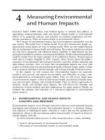
Figure 13.2 shows the distribution of accessibility to jobs in the Baltimore
metropolitan region.

FIGURE 13.2a

Distribution of accessibility to jobs in 1996 in the Baltimore metropolitan
modeling domain.
© 2001 by CRC Press LLC

13.4.3 E

MPIRICAL

E

VIDENCE



ABOUT

M

OBILITY

D

ISPARITY

Mobility increases with income. In 1990, people with household income under
$10,000 traveled 16 mi a day (2.6 trips), less than half the distance by people with
household income of $40,000 and over (38 mi and 3.6 trips) (U.S. DOT 1997b).
The disparities are evident in the percentage of adults holding drivers’ licenses and
vehicle availability: in 1990, households with income under $10,000 had only 73%
of adults holding drivers’ licenses and had only 1 vehicle available, compared with
95% of adults and 2.3 vehicles for households with income $40,000 and over. In
1995, low-income households with income below $25,000 comprised 29% of all
households but accounted for 65% of households without a vehicle.
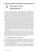
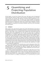
Mobility disparities by race/ethnicity are significant. Regardless of income,
whites travel more than any other races and Hispanics (of all races) (see Figure 13.3).

FIGURE 13.2b

Distribution of accessibility to jobs in 2020 in the Baltimore metropolitan
modeling domain.
© 2001 by CRC Press LLC

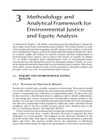
After controlling geographic locations (central city, suburban, and nonmetropolitan
areas), the disparity remains (U.S. DOT 1997b). In 1990, white men in urban areas
traveled 39 mi and made 3.4 trips a day on average, compared with 29.5 mi and 2.8
trips for Hispanic men and 24.1 mi and 3.0 trips for black men (Figure 13.4). In
1995, African Americans took 3.9 trips a day, compared to 4.4 daily trips per person
for whites. Vehicle availability and licensing vary with race/ethnicity. In 1990, whites
had the highest vehicle availability and percentage of adults holding drivers’ licenses.
In 1995, African Americans, while making up 11.8% of all households, accounted
for 35.1% of households without a vehicle (FHWA 1997). This disparity affects the
choice of transportation modes by race/ethnicity. Whites are more likely to make
trips by private vehicle than minorities. In 1990, whites aged 16 to 64 in urban areas
took 92% of their trips by car, compared with no more than 78% for blacks, 81%
for other races, and no more than 82% for Hispanics (Rosenbloom 1995). Blacks
were the most likely to take transit and walking trips, 8% and 12%, respectively,
while whites were the least likely to take transit and walking trips (less than 2% and
5%, respectively). According to the 1995 NPTS data, African Americans made 76%
of their trips by private vehicle, compared with 88% for whites (FHWA 1997).
Conversely, African Americans were more likely to use transit and walking, account-
ing for 7 and 9% of their trips, respectively. Transit share of person trips was only
1% for whites and 3% for Hispanics.

FIGURE 13.3

Average daily travel by race and income level:1990.

Source:

U.S. DOT (Depart-
ment of Transportation, Bureau of Transportation Statistics). Transportation Statistics Annual
Report 1997. BTS97-S-01. Washington, D.C.: U.S. Government Printing Office. 1997b.
© 2001 by CRC Press LLC

13.4.4 A

CCESSIBILITY

D

ISPARITY



AND

S

PATIAL

M

ISMATCH

While evidence about mobility disparity is abundant, accessibility disparity studies
mostly focus on access to jobs and the spatial mismatch hypothesis. For many years,
researchers have observed a clear contrast between the large number of jobs created
in the suburbs and the high unemployment rate in inner city neighborhoods, partic-

ularly among African Americans. This lack of connection between job and residence

FIGURE 13.4

Miles of daily travel: 1990.

Source:

U.S. DOT (Department of Transportation,
Bureau of Transportation Statistics). 1997b. Transportation Statistics Annual Report 1997.
BTS97-S-01. Washington, DC: U.S. Government Printing Office. 1997b.
30
43
39
17
16
11
15
20
24
26
29
32
34
38
© 2001 by CRC Press LLC

locations of potential job seekers has been a topic of debate about the so-called
spatial mismatch hypothesis for three decades. More than 30 years ago, Kain (1968)
found a positive relationship between the fraction of employment held by blacks

and the proportion of black residents in various neighborhoods in Detroit and
Chicago. The fraction of black employment declined with distance from the major
black neighborhoods. From these findings, he believed that residential segregation
contributed to high unemployment rates of blacks in inner cities.
After reviewing 20 years’ empirical evidence on the “spatial mismatch” hypoth-
esis, Holzer (1991) concluded that spatial mismatch had a significant effect on black
employment, but the magnitudes of these effects remained unclear. A rich body of
literature on the spatial mismatch hypothesis has produced mixed results, and
research methodology may contribute to the conflicting findings (Sanchez 1999).
A critical analytical issue in this debate is the measurement of access to jobs.
Commuting time and distance are the most frequently used measures. Gordon,
Kumar, and Richardson (1989) compared average commute time of automobile
commuters by income, race, place of residence, and city-size class. Their results
show that neither nonwhite nor low-income commuters have longer commutes than
others. However, Kasarda (1995) found that blacks had longer commutes than whites
and central city to suburb commute times were exceptionally long for public transit
users, particularly blacks. O’Regan and Quigley (1997) also reported longer com-
mute times for blacks than for other ethnic groups. After controlling for travel modes
and residence and workplace locations, they still found slightly longer commutes
for blacks. These results provide support for the spatial mismatch hypothesis.
Although finding a more than 2-min. longer commute on average for black workers
after controlling other factors, Taylor and Ong (1995) attributed the extra time to
slower travel speed rather than spatial mismatch. Overall, the bulk of research
indicates that most researchers agree that blacks have a longer commute time than
other groups, but they do not agree on what causes the differences or what the policy
and planning implications of the differences in terms of transportation barriers to
job access are (Shen 2000).
Two methodological issues weaken previous research. As discussed above, com-
mute time and distance are poor accessibility measures, and are especially unreliable
measures of relative access to jobs (Sanchez 1999). This inadequacy is worsened

by the use of aggregate data at large geographic levels. Most analyses are based on
the dichotomy of the central city and suburb. Shen (2000) argues that this dichotomy
blurs the spatial variations of accessibility among neighborhoods and particularly
misrepresents that of disadvantaged population groups. Such a spatial bias is evident
in the country’s 20 largest metropolitan areas. In 13 metropolitan areas, workers
residing in the largest poverty enclave in the central city had the longest average
commute times, usually 10% more than the other areas.
An improvement in the recent literature is use of gravity-type accessibility
measures and fine-grained units of analysis. Sanchez (1999) used gravity-type acces-
sibility measures for access to job and a two-stage least-square regression for esti-
mating the relationship between labor participation levels and access to public transit
in Portland, Oregon and Atlanta. He found that access to public transit was a
significant factor in explaining labor participation and provided support for use of
© 2001 by CRC Press LLC

public transportation for addressing the spatial mismatch phenomenon. Shen (2000)
used the general accessibility index based on a gravity formulation and multiple
regression models to explain the variation in commute times. In the Boston metro-
politan area, general employment accessibility was very significant in explaining
variation in commute time; increasing the accessibility index by one standard devi-
ation (0.44) would result in a decrease of the average commute time by 2 min. (0.4
standard deviation). These studies did not show how accessibility measures them-
selves vary by different population groups. There is some evidence that suggests
accessibility disparities vary by race/ethnicity. In Los Angeles, accessibility was
found to be lower for middle-class people than either low- or high-income people
(Wachs and Kumagai 1973).
As mentioned earlier, some metropolitan planning organizations have recently
adopted accessibility, particularly the cumulative-opportunity type, as an equity
measure. The 1998 Regional Transportation Plan (RTP) of the Southern California
Area Governments (SCAG) established eight categories of objectives and perfor-

mance indicators: mobility, accessibility, environment, reliability, safety, livable
communities, equity, and cost-effectiveness (SCAG 1998). As an objective in the
RTP, accessibility is defined as ease of reaching opportunities and measured by
percent of commuters who can get to work within 25 min. For equity evaluation,
the RTP measures accessibility improvement by income and race/ethnicity in two
modes: increased accessibility (trips < 30 min.) by transit and increased accessibility
(trips < 30 min.) by auto. Results show that all groups benefit from increased
accessibility when compared with the baseline scenario. The low-income group
particularly benefits from the improved accessibility due to transit restructuring.
Access is also a priority in the Vision of the National Capital Region Transpor-
tation Planning Board (TPB), an official Metropolitan Planning Organization for the
Washington metropolitan region. To address federal requirements on environmental
justice, TPB staff used accessibility measures to evaluate the 1999 Financially
Constrained Long-Range Transportation Plan (MWCOG 1999). It is cumulative-
opportunity type accessibility, defined as jobs that can be reached by mode (auto,
transit, and the fastest travel mode) within 45 min. The 45-min. travel time captures
78% of the work trips in 2000 and 68% of the work trips in 2020. Results show
that changes in accessibility between 2000 and 2020, as a result of the long-range
plan, will not disproportionately affect low-income and minority populations.

13.5 MEASURING DISTRIBUTIONAL IMPACTS
ON PROPERTY VALUES

Transportation improvements change accessibility, which affects the location choice
of households and firms. These impacts influence distributional patterns of activities.
When making their location decisions, households and firms are willing to pay a
certain amount to satisfy their demand for accessibility. Therefore, property value
reflects the value of accessibility, and transportation investment benefits are capital-
ized in the land market.
Hedonic pricing method, as discussed in Chapter 4, can be used to measure the

implicit price for accessibility. Including an accessibility index in the hedonic price
© 2001 by CRC Press LLC

function would yield an implicit price that households or firms are willing to pay
for a certain degree of accessibility. This analysis involves
• Model specification,
• Variable estimation,
• Model estimation,
• Application of implicit price to analysis zones,
• Segmentation of analysis zones by population groups,
• Tabulation of the distribution of benefits by different groups.
As shown in Chapter 4, the hedonic price function is specified so that the
dependent variable is housing price and the independent variables include structural,
neighborhood, locational, and environmental characteristics. The accessibility index,
as part of location characteristics, can be estimated for highway, transit, or their
combination, using the method discussed previously. If the hedonic function is linear,
the regression coefficients for accessibility variables represent the value of capital-
ized benefits per unit accessibility index. Since various locations have different
degrees of accessibility, applying the regression coefficients to an analysis zone
would give us the total value of capitalized benefits from transportation improve-
ments for that particular zone. These capitalized benefits accrue to the residents in
that particular zone. By analyzing population composition in all analysis zones, we
are able to see how benefits are distributed among population groups.
Sanchez (1998) uses the hedonic price method to examine the distribution of
capitalized transportation benefits within the Atlanta urbanized area. The geographic
unit of analysis is block groups. A gravity-type highway accessibility index is used
to measure the change in highway accessibility associated with the addition of
major highway facilities. The dependent variable is owner-occupied house value
per square foot (median house value for each block group divided by the average
block-group house size from tax assessor’s records). The independent variables

include average house age, highway access, bus access, rail access, percent homes
on public sewer, commercial and industrial land, property tax millage rate, sales
taxes, per capita transit fares, standardized test scores, and student-to-teacher ratio.
Results show that the average per square foot capitalized benefit is about $4.33,
which equivalently represents 6.83% ($7,365) of the total value of the average-
priced house ($107,863). Net transportation benefits have an intrametropolitan
variation; the central city receives the largest benefit while the suburbs obtain the
smallest. The results do not indicate any significant bias toward particular income
or racial groups. Unlike almost all other hedonic studies in the current literature,
this study uses census data rather than armslength sales (i.e., sales not between
people related by kin or business) data.
This type of analysis is useful for evaluating long-range transportation plans
and transportation improvement programs at the metropolitan and regional level.
However, it misses some microlevel impacts associated with transportation
improvements. While transportation improvements benefit houses at large, major
transportation facilities actually depress the property values of those houses in close
proximity. Early studies indicate up to a 10% decline in property value for houses
© 2001 by CRC Press LLC

immediately abutting a freeway, especially an elevated freeway (FHWA 1976).
Homes near freeway interchanges are also sold at a discount. In Alameda and Contra
Costa counties of the San Francisco Bay Area, the 1990 sales price of a home
declined $2.80 and $3.41, respectively, for every meter closer to a freeway inter-
change (Landis and Cervero 1999). On the other hand, new 4-lane roads generally
raise land values by 3% to 5% for houses within a 0.5-mi radius, and the impact
can extend further, as much as 15 mi (National Transit Institute 1998).
Residential property values and rail transit are also positively related. New
transit systems or transit improvements also increase property values along the
transit corridor. Boyce et al. (1972) found that the PATCO rapid transit line between
Philadelphia and Lindenwold had a positive effect on residential property values.

In Portland, Oregon, the average house price within a 500-m walking distance of
selected light-rail stations was 10.6% ($4,300) higher than that of houses within
the study area but beyond 500 m (Al-Mosaind, Dueker, and Strathman 1993). A
hedonic price model reports a statistically weak negative price gradient with
respect to distance for houses within 500 m ($21.75 per m from a station). A much
lower price gradient was reported for houses near BART stations in San Francisco
(Landis and Cervero 1999). Homes near BART stations command a premium of
$2.29 per m from the nearest BART station (measured along the street network)
in Alameda County and $1.96 in Contra Costa County. In Washington, D.C., Metro
generated considerable land rent premium; these premiums were most dramatic
in older, more deteriorated sections of downtown (Rybeck 1981). In Atlanta,
elevated heavy-rail stations increased housing prices in lower-income neighbor-
hoods nearby but decreased house prices in a higher-income neighborhood (Nelson
1992). The findings indicate that the balance of benefits and costs associated with
proximity to an elevated transit station might manifest itself differently depending
on the neighborhoods.
Evidence also shows positive impacts of transit on commercial property values
adjacent to transit stations, although it is more sketchy than the residential literature.
In the Midtown MARTA station area of Atlanta, the sales price per square meter of
commercial buildings declined by $75 for each meter away from the center of transit
stations and increased by $443 for location within special public interest districts
(Nelson 1998). In Washington, D.C., Metro generated commercial rent premium of
$2 per square foot for prime blocks that had a Metro station entrance or were across
the street from one and $1 per square foot for blocks adjoining prime blocks (Rybeck
1981). In Santa Clara County, the lease premium was 3.3 cents per square foot for
properties within 0.25 mi of a light-rail station and 6.4 cents per square foot for
those between 0.25 and 0.5 mi (Weinberger 2000). The sales premiums were $8.73
and $4.87 per square foot, respectively.
Clearly, these capitalized benefits or costs can happen at the microscale, station-
specific level. Therefore, equity impact assessment of these types requires a more

fine-grained unit of analysis than the regional level. It appears that it is necessary
to go to the block level, even the parcel level to detect these microscale impacts. A
GIS-based methodology is essential. In particular, GIS can be used to geocode the
exact locations of sales transactions, to measure the distance to the nearest transit
stations and to the nearest freeway interchanges, to identify property parcels along
© 2001 by CRC Press LLC

the roadway, to estimate socioeconomic data at the fine scale using data at the larger
geographic units, and to estimate accessibility measures.

13.6 MEASURING ENVIRONMENTAL IMPACTS

In Chapters 8 and 9, we discussed the integration of urban and environmental models
in a GIS environment. This integration serves as a framework for evaluating the
environmental impacts of transportation systems, projects, plans, and programs on
different population groups. This methodology follows a sequential process (Table
13.4). Land and transportation models generate data about traffic speed, traffic
volume, and vehicle trips, which are input to emission modeling, air quality mod-
eling, and noise modeling. Ambient pollutant concentration and noise level data,
which are produced from air quality and noise models, are then processed in a GIS
environment and displayed as contour lines. By overlaying these contour lines with
the distribution of protected populations, we are able to see the distributional impacts
of transportation projects, plans, and programs.
A few analytical issues need the analyst’s attention. First, it is essential to use
a fine geographic unit of analysis to uncover some environmental impacts of trans-
portation on different segments of population (Forkenbrock and Schweitzer 1999).
As discussed earlier, air pollution and noise from transportation are generally con-
strained by the proximity of transportation facilities. Line-source dispersion models
usually predict pollutant concentrations in the vicinity of highway; for example,
CAL3QHCR predicts air pollutant concentrations in receptors located within 150

m of the roadway (Benson 1994). Just like measuring property value impacts,
measuring differential environmental impacts requires demographic data at a fine
unit of geography, such as the census-block level.
Second, sociodemographic data may not be available at the fine geographic unit,
and assumptions and alternative data sources have to be used. At the census-block
level, we still have to assume that population is homogeneous within a census block.
As we know, the first row of houses abutting the roadway bears the brunt of adverse
environmental impacts. This fact makes some researchers wonder whether it is
necessary to use parcel level data. With the help of GIS and property databases,
those houses adjacent to the roadways can be identified. However, demographic data
are not available at the parcel level. If the study area is small, these data can be
obtained through a survey. A large study area may preclude data collection through
a survey due to budget constraints. Instead, some statistical methods may be used
to derive estimates for a smaller geographic unit from available data at a larger
geographic unit.
Third, while some transportation-related environmental impacts are localized
such as carbon monoxide, others have a regional scope such as ozone. Reactive
pollutants such as ozone and its precursors nitrogen oxides and VOCs are modeled
differently from inert pollutants. Nitrogen oxides and VOCs themselves have health
impacts. The modeling domain for ozone often covers a few states, while land-use
transportation modeling often operates at the metropolitan area level. The analyst
needs to develop an interface among different modeling domains and units of
analysis for integrating urban and environmental models.
© 2001 by CRC Press LLC

13.7 EQUITY ANALYSIS OF TRANSPORTATION POLICIES

A large body of literature on welfare economics and public finance deals with public
policies, or primarily the distribution of costs and benefits incurred by taxes and
public infrastructure and services.

Transportation infrastructure and services are funded by a variety of taxes such
as federal and state fuel gasoline tax, state use fees, state sales tax, local sales tax,
federal and state income tax, and property tax. Giuliano (1994) reviews the literature

TABLE 13.4
Integrating Urban Models, Environmental Models, and GIS
for Transportation Equity Analysis

Modeling Input Output
Examples of Modeling
Packages

Land-use/Transportation
Modeling
• Land-use model
• Vehicle availability
• Trip generation
• Trip distribution
• Modal split
• Trip assignment
Socioeconomic data
Land-use data
Transportation network
and database
VMT
Vehicle trips
Travel speed
Traffic volume
ITLUP
(DRAM/EMPAL)

MEPLAN
TRANUS
TP+ (MINUTP)
TRANPLAN
TransCAD
Emission Modeling Traffic mix
Traffic speed
Temperature
Precipitation
Vehicle emission
factors
MOBILE
EMFAC (California)
Air Quality Modeling Emission factors
Traffic speed
Traffic volume
Queue lengths
Lane widths
Wind speed
Wind direction
Ambient
pollutant
concentration
ISC3
PART5
AP-42
CALINE, such as
CAL3QHCR
Noise Modeling Traffic volume
Traffic mix

Traffic speed
Noise level STAMINA
Human Exposure
Modeling
Human activity patterns
Ambient pollutant
concentration
Exposure Human Exposure Model
SHAPE
REHEX
GIS Ambient pollutant
concentration
Noise level
Exposure
Transportation network
Census geography
Census data
Spatial
relationship
between
environmental
quality/exposure
and population
groups
ArcView/ArcInfo
MapInfo
TransCAD/Maptitude
© 2001 by CRC Press LLC

on the incidence of taxes that are used to fund highway infrastructure and services.

She concludes that these taxes are regressive overall.
The clash between some mainstream environmental and environmental justice
groups and between environmental and equity goals is demonstrated in various
road pricing or value pricing proposals. Economists and some environmental
groups argue that auto driving has been underpriced and subsidized and does not
account for external costs caused by driving. To combat air pollution problems
that have eluded any solution in many metropolitan areas, they have proposed a
variety of pricing mechanisms such as congestion pricing, tolls, Pay-As-You-Drive
insurance, and VMT charges. They believe that these mechanisms will force drivers
to face the true cost of driving and reduce the bias toward overconsumption of
driving. Environmental justice groups fear that these mechanisms would price the
poor and often people of color out of roads. Another argument against road pricing,
like State Route 91 in southern California, is that it will encourage sprawl because
any relief in congestion as a result of pricing mechanism will facilitate the rich
moving further away.
Many believe that congestion and other pricing policies are not necessarily
regressive. One reason is that peak period drivers tend to be overwhelmingly middle-
and upper-income people (Hattum 1996; Lee 1989). In San Francisco and Minne-
apolis, low-income drivers account for just 2% and 3%, respectively, of commuter
trips (Komanoff 1996). Another argument for congestion and other pricing mecha-
nism is that they will reduce traffic congestion, air pollution, and automobile depen-
dency and, thereby, benefit the low-income population. In particular, as discussed
in Chapter 10, studies have shown that a low-income population tends to be exposed
to a higher degree of air pollution nationwide.
Cameron (1994) evaluates efficiency and equity of existing transportation
systems and a 5-cent-per-mile VMT in Southern California. The study measures
transportation benefits by five income groups using the willingness-to-pay meth-
odology. Transportation costs by income groups include automobile expenses
(ownership, maintenance, fuel, and insurance), transit fares, transportation taxes
and fees, health costs of air pollution, and traffic congestion costs. The distribution

of net transportation benefits (benefits minus costs) for the current transportation
systems is regressive: the lowest income group receives $650 (6% of the regional
total), the lower-middle income group receives $1,430, the middle-income group
receives $1,980 (19% of regional total), the upper-middle-income group receives
$2,880, and the upper-income group receives $3,750 (35% of the regional total).
Comparing it with personal income distribution, the current transportation system
redistributes transportation benefits toward those in the middle. A 5-cent-per-mile
VMT fee would make each income group better off: an increase in net transpor-
tation benefits from $90, $150, $180, $250, to $420, respectively, for the lowest-
income to the highest-income group. This result is subject to a wide band of
uncertainty because of highly debatable assumptions about the value of travel,
time, and health. The author concludes that the result is plausible for the upper
three, perhaps four, income groups, but highly questionable for the lowest income
group (Cameron 1994). From the utilitarian perspective, this policy proposal is
desirable since everyone seems to be better off. However, it aggregates the existing
© 2001 by CRC Press LLC