Ecological Modeling in Risk Assessment - Chapter 11 potx

© 2002 by CRC Press LLC
CHAPTER 11
Landscape Models — Aquatic and Terrestrial
Christopher E. Mackay and Robert A. Pastorok
In contrast to ecosystem models, which are spatially aggregated models, landscape models are
spatially explicit models that may include several types of ecosystems. In landscape models, the
values of one or more state variables are dependent upon either distance or relative location. A
landscape model may be totally constructed on a spatial basis, such as cellular automata models
using a GIS platform. Some ecosystem models can be easily applied in a landscape mode. For
example, AQUATOX is currently being applied to the Housatonic River in Connecticut by dividing
the model into discrete segments and linking results from each segment to input information for
downstream segments (Beach et al. 2000). Thus, models like AQUATOX and CASM were consid
-
ered in the development of recommendations for landscape models.
Example endpoints for landscape models include:
• Spatial distribution of species
• Abundance of individuals within species or trophic guilds
•Biomass
• Productivity
• Food-web endpoints (e.g., species richness, trophic structure)
• Landscape structure indices (Daniel and Vining 1983; FLEL 2000a,b; Urban 2000)
We review the following landscape models (Table 11.1):
• Marine and Estuarine
• ERSEM (European regional seas ecosystem model), a model of marine benthic systems (Eben-
hoh et al. 1995; Baretta et al. 1995)
• Barataria Bay ecological model, a model of an estuary (Hopkinson and Day 1977)
• Freshwater and Riparian
• CEL HYBRID (coupled Eulerian LaGrangian HYBRID), a coupled chemical fate and ecosys-
tem model for lakes and rivers (Nestler and Goodwin 2000)
• Delaware River Basin model, a segmented river model (Kelly and Spofford 1977)
• Patuxent River Watershed model, a whole watershed model comprising ecological and economic

systems (Voinov et al. 1999a,b; Institute for Ecological Economics 2000)
1574CH11.fm Page 149 Tuesday, November 26, 2002 6:10 PM
© 2002 by CRC Press LLC
Table 11.1 Internet Web Site Resources for Aquatic and Terrestrial Landscape Models
Model Name Description Reference Internet Web Site
ERSEM A marine benthic ecosystem model for European
regional seas
Ebenhoh et al. (1995); Baretta et al. (1995)
~wwwem/res/ersem.html
Barataria Bay ecological
model
An early generation model of an estuarine system Hopkinson and Day (1977) Updated models at:
/>CEL HYBRID Models that combine population dynamics with
detailed fate modeling for toxic chemicals
Nestler and Goodwin (2000) />Delaware River Basin
model
A spatially explicit model of a river system Kelly and Spofford (1977) />Patuxent River watershed
model
A watershed model incorporating human interactions Voinov et al. (1999a,b); Institute for Ecological
Economics (2000)
/>AT LSS A landscape modeling system for the Everglades with
specific modeling approaches tailored to each trophic
level
DeAngelis (1996)
/>Disturbance to wetland
vascular plants model
A spatially explicit model for predicting the impacts of
hydrologic disturbances on wetland community
structure
Ellison and Bedford (1995)

ellisoncv.html
LANDIS A landscape model for describing forest succession
over large spatial and temporal scales
Mladenoff et al. (1996); Mladenoff and He
(1999)
/>FORMOSAIC A cellular automata landscape model Liu and Ashton (1998)
liu1999.htm
FORMIX A landscape model for a tropical forest Bossel and Krieger (1991) />ZELIG A forest landscape model with probabilistic mortality
functions
Burton and Urban (1990)
bhs/Models/Zelig.html
/>JABOWA A highly developed landscape model for mixed species
forests
Botkin et al. (1972); West et al. (1981); Botkin
(1993a,b)
/>
model_db/mdb/jabowa.html
Regional landscape model A model for evaluating the impact of ozone exposure
upon forest stands and associated water bodies
Graham et al. (1991) N/A
Spatial dynamics of
species richness model
A model for evaluating the effects of habitat
fragmentation on species richness
Wu and Vankat (1991) N/A
STEPPE A gap-dynamic model of grassland productivity Coffin and Lauenroth (1989); Humphries et al.
(1996)

model_db/mdb/steppe.html
Wildlife-urban interface

model
A vegetation cover and wildlife habitat utilization model
for evaluating the impacts of urban development
Boren et al. (1997) N/A
SLOSS A model of nestedness of species assemblages in
habitat patches of varying size
Boecklen (1997) N/A
Island disturbance
biogeographic model
A model for evaluating the effects of perturbations on
the distribution of species within a series of linked
island habitats
Villa et al. (1992)
bio345-01/biogeo.htm

island_biogeography.html
Multiscale landscape
model
A model of landscape structure based on the
probability of species occurrences
Johnson et al. (1999)
richards.html
Note: N/A - not available
1574CH11.fm Page 150 Tuesday, November 26, 2002 6:10 PM
© 2002 by CRC Press LLC
•Wetland
• ATLSS (across-trophic-level system simulation), a landscape model of the Everglades (see
DeAngelis 1996)
• Disturbance to wetland vascular plants model, a model of wetland plant communities (Ellison
and Bedford 1995)

•Forest
• LANDIS (landscape disturbance and succession), a forest landscape model along with the
following four models (Mladenoff et al. 1996; Mladenoff and He 1999)
• FORMOSAIC (forest mosaic) model (Liu and Ashton 1998)
• FORMIX (forest mixed) model (Bossel and Krieger 1991)
• ZELIG (Burton and Urban 1990)
• JABOWA (Botkin et al. 1972; West et al. 1981; Botkin 1993a, b)
• Regional landscape model, a model of ozone effects on a forest and associated water bodies
(Graham et al. 1991)
• Spatial dynamics of species richness model, a model to evaluate the effects of habitat fragmen-
tation (Wu and Vankat 1991)
•Grassland
• STEPPE, a gap-dynamic model of grassland productivity (Coffin and Lauenroth 1989;
Humphries et al. 1996)
• Wildlife-urban interface model, a model to predict the effects of human activities on wildlife
(Boren et al. 1997)
•Island
• SLOSS (single large or several small), a model of distribution of species assemblages in habitat
patches (Boecklen 1997)
• Island disturbance biogeographic model, a model of species distributions within linked island
habitats (Villa et al. 1992)
• Multi-scale
• Multi-scale landscape model, a model of landscape structure based on probability of species
occurrences (Johnson et al. 1999).
ERSEM
ERSEM was developed as a comprehensive model of carbon dynamics and major nutrients (nitro-
gen, phosphorus, silicon) along the coastal shelf of the North Sea (Ebenhoh et al. 1995; Baretta et
al. 1995). The model represents the North Sea as a set of “geographical boxes” that describe regional
differences in physical, chemical, and biological characteristics in one to three dimensions. The
model consists of pelagic, benthic, and transport submodels. The pelagic submodel includes pop

-
ulations of phytoplankton, zooplankton, and fishes representative of the regions. The benthic
component of the model is connected to the pelagic production dynamics by the settling of pelagic
detritus and sinking diatoms. The benthic submodel emphasizes the biology of the benthic organ
-
isms, the functional importance of bioturbation, and the role of nutrient profiles in regulating
microbial activity. The biological populations are based on the concept of functional groups with
common processes such as food intake, assimilation, respiration, mortality, and nutrient release but
with different parameters for each group.
ERSEM has been used to examine the functional dependence of the benthic system on inputs
from the pelagic system, the importance of predation as a stability-conferring process in model
subsystems, and the importance of detritus recycling in the benthic food web. The kinds of data
inputs needed for ERSEM include annual cycles of monthly mean (or median) values together with
ranges of variability, time series of river input of dissolved and particulate nutrient loads for all
continental rivers, time series of daily water flow across the borders of horizontal compartments,
time series of solar irradiance, and time series of boundary conditions for nutrients.
1574CH11.fm Page 151 Tuesday, November 26, 2002 6:10 PM
© 2002 by CRC Press LLC
Realism — HIGH — The overall spatial structure and detailed physical, chemical, and biological
components of ERSEM suggest that the model provides a realistic description of major features of
the North Sea.
Relevance — HIGH — The endpoints for modeled organisms in both the pelagic and benthic submodels
are useful for assessing ecological impacts and risks posed by chemical contaminants. Although the
model does not explicitly account for toxic chemical effects, several parameters could be adjusted
by the user to implicitly model toxicity.
Flexibility — MEDIUM — The modeling framework has been developed for the North Sea. However,
the geographical-box model approach might be adapted for other similarly scaled marine systems.
Treatment of Uncertainty — LOW — ERSEM has not been the subject of detailed sensitivity or
uncertainty analyses.
Degree of Development and Consistency — MEDIUM — The development of ERSEM as a set of

coupled submodels might lend the model to application to other systems. The model has been
implemented, and a software version is probably available from the authors.
Ease of Estimating Parameters — MEDIUM — The model has a considerable number of physical,
chemical, and biological parameters to estimate. However, the parameters have fairly understandable
interpretations that can facilitate estimation.
Regulatory Acceptance — LOW — ERSEM was constructed to evaluate impacts of nutrients intro-
duced to the North Sea. The model has regulatory applicability, but the reference did not specifically
mention any U.S. or international regulatory use or acceptance.
Credibility — MEDIUM — Model calibration and model:data comparisons suggest that the model
captures some of the key ecological dynamics characteristic of the North Sea. However, few
published references to the model exist, and the number of actual users is unknown but presumably
fewer than 20.
Resource Efficiency — LOW — The spatial nature of the model, combined with the food-web detail
in the pelagic and benthic submodels, suggests that the model would require a major commitment
of resources to implement for specific case studies.
BARATARIA BAY MODEL
The Barataria Bay model is an early generation model that describes carbon and nitrogen flows
within an open estuarine ecosystem (Hopkinson and Day 1977). Although the state variables are
not directly distinguished with regard to space, transfer coefficients representing fluxes between
model compartments are distance-dependent. Seven state variables are tracked for carbon (bio
-
mass) and nine state variables for nitrogen (rate-limiting nutrient). Living marsh plants are
modeled as the dominant species, Spartina alterniflora. The nonmarsh plants consist almost
exclusively of phytoplankton. Two separate detrital communities were modeled, one in association
with a marsh, and one in association with the open marine environment. Both include not only
litter material but also associated decomposing organisms such as bacteria and fungi. Both also
exhibit similar dynamics because detritus from higher-level marsh plants is transported by tidal
action from the marsh into the marine environment. Therefore, differences between the two
detrital communities were primarily due to differing relative amounts of plankton, zooplankton,
and high-level plant material inputs. A single state variable for marsh fauna accounted for insects,

raccoons, muskrats, birds, snails, crabs, and mussels. Similarly, the state variable for marine
fauna accounted for all fish.
Transfer relationships between the state variables are based on steady-state kinetics. Estimates
of transfer coefficients were calculated as the product of the compartment capacity (e.g., biomass
of zooplankton) at equilibrium and the modeled rate of change in capacity.
Realism — LOW — The Barataria Bay model uses a rudimentary approach to modeling landscape
effects by embedding the spatial constituents within the underlying algorithm. This embedding was
done by spatially defining all of the state variables and thus making the transfer coefficients distance-
1574CH11.fm Page 152 Tuesday, November 26, 2002 6:10 PM
© 2002 by CRC Press LLC
dependent. Generalized definitions of state variables such as marsh fauna and marine fauna make
the model less realistic than similar models. Results from simulations indicate that this aggregation
has the greatest effect on the model’s overall realism.
Relevance — LOW — The Barataria Bay model primarily describes the dynamic flows of carbon and
nitrogen in the estuarine environment. Because food-web components are highly aggregated in this
model, it has limited relevance for ecological risk assessment of toxic chemicals.
Flexibility — LOW — The Barataria Bay model is the least flexible of the aquatic landscape models.
Its inherent structure defines fixed spatial compartments within the model. Moreover, its steady-
state approach to defining the major state variables limits applications.
Treatment of Uncertainty — LOW — Neither uncertainty nor variability was tracked in the execution
of this model.
Degree of Development and Consistency — MEDIUM — The model was not validated. Although
this model was developed as software, no indication exists as to its availability. However, Hopkinson
and Day (1977) provide sufficient details for programming and application of the model.
Ease of Estimating Parameters — LOW — The Barataria Bay model is fairly complex and must be
parameterized with empirical data.
Regulatory Acceptance — LOW — To our knowledge, the model does not have any regulatory status
and has not been applied in a regulatory context.
Credibility — MEDIUM — The Barataria Bay model depends on very fundamental modeling tech-
niques and contains no mechanistic functions.

Resource Efficiency — HIGH — The model was deemed efficient to implement because, although it
is heavily parameterized, the parameters are estimated on the basis of steady-state conditions.
CEL HYBRID
CEL HYBRID is a spatially explicit model for aquatic ecosystems developed by researchers at the
U.S. Army Corps of Engineers (Nestler and Goodwin 2000). This model attempts to join the
disparate mathematical approaches of population dynamics with chemical fate modeling. The idea
is to integrate biological functions and physical processes by using a mixed-modeling framework.
The approach includes a semi-Lagrangian model (Priestly 1993) in which physical and chemical
processes are modeled on a Eulerian grid and biological organisms are modeled with a separate
individual-based model (Figure 11.1
). The points of connection between the two systems update
times at which localized biomasses representing organisms are integrated (or perhaps appropriately
averaged) over the spatial grid. This approach permits the representation of real feedback between
the chemistry and the biology. An individual-based population model is a specific example of the
broader CEL HYBRID approach to modeling. What individual-based modeling does for population
modeling, CEL HYBRID does for ecosystem modeling (Nestler 2001, pers. comm.).
The modeling strategy inherent in CEL HYBRID has subtle problems in maintaining conser-
vation when any sources or sinks are present and a problem with inflation of error when the two
time-steps are not identical. It would be useful to somehow enable the individual-based component
to handle extremely large numbers of individuals, such as might be necessary for fish in reservoirs.
Supercomputing might facilitate this, but the solution might eventually involve hybridizing the
individual-based approach with a frequency-based model in which some “individuals” are really
exemplars that represent an entire class of similar organisms.
Realism — HIGH — CEL HYBRID could incorporate key population-dynamic and chemical processes,
including density dependence, physical transport (for both chemicals and organisms), chemical
uptake, bioaccumulation, and toxicant kinetics. Because the model has not been fully articulated,
we cannot assess the number of assumptions it requires.
Relevance — HIGH — CEL HYBRID provides output that is directly relevant to the endpoints used
in population-level ecotoxicological risk assessment. Several parameters can be used to describe the
ecosystem-level impacts of toxic chemicals.

1574CH11.fm Page 153 Tuesday, November 26, 2002 6:10 PM
© 2002 by CRC Press LLC
Flexibility — HIGH — CEL HYBRID could permit alternate formulations of the dose–response
functions. It could also support several different models of population growth. The model should
be applicable to a wide variety of organisms in different environments.
Treatment of Uncertainty — LOW — In principle, one could introduce uncertainty and risk analysis
into CEL HYBRID by enclosing the model within a Monte Carlo shell. However, the computation
costs for this approach are likely to be quite high.
Degree of Development and Consistency — LOW — The inner workings of CEL HYBRID are fairly
difficult to understand. The model has not yet been implemented in software. The programming
effort needed for this task is considerable. Nevertheless, elementary feasibility and consistency
checks would be simple to implement.
Ease of Estimating Parameters — LOW — The effort needed to estimate parameters for CEL
HYBRID (once they have been specified) could be substantial.
Regulatory Acceptance — MEDIUM — The model is being developed by scientists at the U.S. Army
Corps of Engineers, which is a regulatory agency. Although the model has not yet been used, it will
likely be supported and used by the U.S. Army Corps of Engineers in the future.
Credibility — LOW — CEL HYBRID is unknown in academia; few publications describe the approach
and, as yet, the model has no applications.
Resource Efficiency — LOW — Applying CEL HYBRID to a particular case would require program-
ming, testing, debugging, and data collection.
DELAWARE RIVER BASIN MODEL
The Delaware River Basin model is a spatially segmented river model designed to evaluate effects
of nutrients and toxic chemicals, specifically phenolic compounds (Kelly and Spofford 1977). As
a segmented river model, the environmental conditions in the upstream reaches affect conditions
in successive downstream reaches. The reaches within the model are treated as homogeneous mixed
water bodies with net active water flow serving as the only link between regions. The model is
Figure 11.1 Structure of the CEL HYBRID Model. (From Nestler and Goodwin (2000) Simulating Population
Dynamics in an Ecosystem Context Using Coupled Eulerian-Lagrangian Hybrid Models (CEL
HYBRID Models). ERDC/EL TR-00-4, U.S. Army Engineer Research and Development Center,

Vicksburg, MS.)
1574CH11.fm Page 154 Tuesday, November 26, 2002 6:10 PM
© 2002 by CRC Press LLC
structured as a generalized compartment model using differential equations describing rates of
change in state variables. Because the principal application of the model was within a static
economic framework, all relationships were designed to describe steady-state conditions.
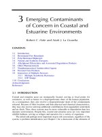
Biotic compartments within the model are defined as trophic levels to allow evaluation of
toxicological impacts on ecologically relevant endpoints such as biomass of primary producers,
herbivores (zooplankton), omnivores (fish), and decomposers (bacteria) (Figure 11.2
). Abiotic
parameters, specifically nitrogen, phosphorus, organic matter, and dissolved oxygen, are included
as inputs to functions regulating the rates of transfer of matter or energy among the principal
biological state variables. The other state variables, phenolic toxicants and temperature, are included
as extrinsic factors affecting the biotic systems.
Aside from primary producers, the definition of the biomass at each trophic level depends on
two main processes in each reach. The first is direct input from upstream reaches. The second is
accumulation of biomass as a result of ingestion and carbon accumulation. This second input
depends on prey availability, predator population size, temperature, and oxygen concentration, as
well as the concentration of toxic chemicals. For the most part, functions were empirically derived
as either exponential or inverse relationships. Other processes that limited biomass accumulation
were respiration, death, excretion, predation, and loss downstream. Rates of predation depend upon
the relative population sizes of each predator and prey pair.
To model primary producers, the rate of nutrient uptake is determined on the basis of two
concurrent Michaelis–Menton relationships (one for phosphorus and one for nitrogen), both mod
-
ified by coefficients dependent on the availability of light in the water column. Light availability
in turn depends on surface-level radiation, water turbidity, and the water depth profile. Grazing
rates are modeled as a function of the abundance of primary producers, the abundance of consumers,
and the individual consumers’ ingestion rates.
Concentrations of toxic chemicals in biota depend on empirical determinations of uptake and

release rates. Release rates are inversely proportional to a concentration-dependent detoxification
rate. The derivation of the exposure–response relationship to account for toxicity was not discussed.
Realism — MEDIUM — The Delaware River Basin model simulates transfer of mass, nutrients, and
energy between trophic guilds on the basis of spatial locations. The relationships defined in the
model appear adequate to account for the main ecological interactions. The assumption of homo
-
geneity within each river reach requires careful differentiation of river reaches under real environ-
mental conditions.
Relevance — HIGH — The Delaware River Basin model is specifically designed to evaluate the effects
of toxic chemicals on biomass at various trophic levels (Figure 11.3). The model has been param
-
eterized for phenolic compounds.
Flexibility — HIGH — The model uses a river reach structure and therefore could potentially be applied
to other riverine ecosystems.
Treatment of Uncertainty — LOW — Neither uncertainty nor variability is tracked in the structure
of the Delaware River Basin model.
Degree of Development and Consistency — MEDIUM — Although the Delaware River Basin model
was developed as software, its availability is unclear. However, Kelly and Spofford (1977) provide
sufficient details to program and apply the model. No validation of the model was done.
Ease of Estimating Parameters — LOW — The Delaware River Basin model requires separate
parameterization for each of the river reach units that compose the landscape. Furthermore, almost
all modifying relationships acting upon the biological state variables are empirically derived. There
-
fore, it is considered to be highly data intensive.
Regulatory Acceptance — MEDIUM — The model was developed as part of the Delaware River
Basin Commission’s Resources for the Future research program. However, there is no indication in
the cited reference or on its Internet web site that it was used within a regulatory context.
Credibility — MEDIUM — The Delaware River Basin model is the product of a history of development
of aquatic trophic-interaction models. However, there is no information about its acceptance or future
development.

1574CH11.fm Page 155 Tuesday, November 26, 2002 6:10 PM
© 2002 by CRC Press LLC
Resource Efficiency — HIGH — The Delaware River Basin model is considered to be among the
most efficient of the aquatic landscape models because of the relatively limited number of parameters
and comparatively simple structure.
PATUXENT WATERSHED MODEL
Voinov et al. (1999a, b) developed a spatially explicit model of the Patuxent River watershed (see
also Institute for Ecological Economics 2000). The major model components include a land-use
conversion submodel, a hydrology model, and an ecological model that consists of nutrient,
macrophyte, consumer, and detritus submodels. Submodels also have been developed to examine
production dynamics in forested and agricultural components of the watershed. The model is used
to address questions about the dynamic linkages between land use and the structure and function
of terrestrial and aquatic ecosystems, the role of natural and anthropogenic stressors and how their
effects change with scale, and the economic effects of alternative management strategies and
policies.
Figure 11.2 Structure of the Delaware River Basin model. (From Kelly and Spofford (1977). Application of an
ecosystem model to water quality management: the Delaware estuary. Chapter 18. In Ecosystem
Modeling in Theory and Practice. C.A.S. Hall and J.W. Day, Jr., (Eds.). John Wiley & Sons, New
York. With permission.)
1574CH11.fm Page 156 Tuesday, November 26, 2002 6:10 PM
© 2002 by CRC Press LLC
The Patuxent model subdivided the watershed into a set of individual landscape units linked
within a GIS, and the submodels are set up for each of these spatial units. The Patuxent model has
been implemented in an integrated simulation system called the Spatial Modeling Environment.
Spatial scales can be specified as 200 m or 1 km. The different submodel components are calibrated
independently at spatial and temporal scales of resolution corresponding to scaled data sets.
Within the Patuxent model, the general ecosystem model (GEM) (Fitz et al. 1996) is designed
to simulate a variety of ecosystem types using a fixed structure across a range of scales (Institute
for Ecological Economics 2000). GEM predicts the response of macrophyte and algal communities
to simulated levels of nutrients, water, and other environmental inputs determined from outputs of

algorithms for upland, wetland, and shallow-water habitats. It explicitly incorporates ecological
processes that determine water levels, plant production, nutrient cycling associated with organic
matter decomposition, consumer dynamics, and fire. Biomass values of producers and consumers,
as well as phosphorus and nitrogen, can be simulated on an annual time scale for different land-
use categories. GEM is essentially an ecosystem model that can simulate system dynamics for a
single homogenous habitat. GEM is replicated throughout the framework of the overall grid-based
model using different parameter sets for each habitat to create the landscape-level analysis. The
developers used a basic version to simulate the response of sedge and hardwood communities to
varying hydrologic regimes and associated water quality.
GEM expresses the dynamics of various ecological processes as the interaction between state
variables (biological stocks) and flows of material, energy, and information (Institute for Ecological
Economics 2000). Vertical or within-cell dynamics are simulated, and the landscape modeling
program processes the results of the unit models. The spatial model calculates the exchange of
material between grid cells and simulates temporal changes in water availability, water quality, and
landscape structure related to habitat or ecosystem type. For each grid cell, a successional algorithm
redefines the habitat/ecosystem type of cells as conditions change and selects parameter sets as
necessary. Ecosystem functions and parameters for each grid cell are determined by the cell’s land
use or habitat designation at the beginning of any simulation time-step. The ecological processes
Figure 11.3 Example output of the Delaware River Basin model. Note: Vertical bars show variability for data.
(From Kelly and Spofford (1977). Application of an ecosystem model to water quality management:
the Delaware estuary. Chapter 18. In Ecosystem Modeling in Theory and Practice. C.A.S. Hall
and J.W. Day, Jr., (Eds.). John Wiley & Sons, New York. With permission.)
1574CH11.fm Page 157 Tuesday, November 26, 2002 6:10 PM
© 2002 by CRC Press LLC
and fluxes are calculated according to that land use and the values of the state variables at that
time for the cell. Human activities can affect the system simulation through the land-use designation
of a cell or through the ecological processes that occur within a cell conditioned on its land use.
Realism — HIGH — The Patuxent watershed model considers the hydrological, biological, economic,
and spatial factors that are important for describing the ecological characteristics of the watershed.
Relevance — HIGH — The ecological populations and endpoints that are represented in the Patuxent

watershed model are of concern and are commonly represented in ecological risk assessments.
Although the model does not explicitly account for toxic chemical effects, several parameters could
be adjusted by the user to implicitly model toxicity.
Flexibility — MEDIUM — The model was developed specifically for the Patuxent watershed. However,
the general ecosystem model that provides the main ecological component (GEM) of this overall
modeling construct could be applied to other aquatic ecosystems.
Treatment of Uncertainty — MEDIUM — Sensitivity and uncertainty analyses have been done on
some parts of the Patuxent watershed model; submodel components could be placed in a Monte
Carlo uncertainty analysis framework.
Degree of Development and Consistency — HIGH — The Patuxent watershed model is highly
developed and can be accessed on the Internet. It is well documented with examples of applications.
Ease of Estimating Parameters — MEDIUM — Given the spatial detail of the Patuxent watershed
model, many parameters for a wide range of physical, chemical, and biological processes are required
to run the full model. The parameters in general have clear process-level meaning, and many might
be estimated from the data usually available for well-studied watersheds.
Regulatory Acceptance — LOW — The Patuxent watershed model was developed by an educational
institution. No reference was made to regulatory acceptance or recommendation.
Credibility — MEDIUM — Results from individual model components were comparable for the most
part with observed data for the Patuxent, but no reported results from implementation of the full
model were available. The Patuxent watershed model is a modified version of the coastal landscape
simulation model developed by Costanza et al. (1990).
Resource Efficiency — LOW — Applications to case studies that did not directly involve the Patuxent
watershed would require substantial efforts in parameter estimation. However, major reprogramming
efforts probably would not be required.
ATLSS
ATLSS is a multicomponent modeling framework for the Florida Everglades that is constructed in
a cellular automata format (DeAngelis 1996). ATLSS is a set of integrated models that simulate
the hierarchy of whole-system responses across all trophic levels and across spatial and temporal
scales that are ecologically relevant to a large wetland system like the Everglades (Figure 11.4).
ATLSS uses different modeling approaches tailored to each trophic level, including differential

equations for process models of lower levels and age-structured and individual-based models for
higher levels. Much of ATLSS was developed on the basis of empirical data for the Everglades.
In ATLSS, process models are used for modeling lower trophic levels (periphyton and macro-
phytes, detritus, micro-, meso- and macroinvertebrates), with a series of differential equations
defining state variables for biomass of various taxonomic or functional groups. To account for
seasonality, the growth and death parameters vary sinusoidally over the year. This allows the system
to respond differentially to perturbations occurring during different times of the year. No functions
in the process models represent predation losses of plant or macroinvertebrate biomass. Rather,
such consumption is considered a separate state variable calculated by modules that describe these
higher trophic-level consumers. The amount of material consumed is subtracted from the appropriate
state variables in a lower trophic module before its next iteration.
In the detritus model, the generation of detritus is proportional to the death term in the primary
productivity module. The disappearance of detritus is proportional to the current stock of detritus
modified by a seasonal coefficient. The growth of the invertebrate group is assumed to vary with
1574CH11.fm Page 158 Tuesday, November 26, 2002 6:10 PM
© 2002 by CRC Press LLC
the product of this group’s own populations and the plant or detritus stocks upon which they graze.
As with the plant models, death varies with the square of their respective stocks, thereby keeping
their populations constrained.
Age-structured population models are used to simulate intermediate trophic levels consisting
of five functional groups of macroinvertebrates and fishes (see review of ALFISH in Chapter 7,
Population Models — Metapopulations). Each spatial cell within the landscape is assumed to be
homogeneous, with a certain carrying capacity for macroinvertebrates and fish, as determined by
the process module. Mature individuals of each functional group produce a set number of viable
offspring during their reproductive season. Baseline age-dependent mortality is assigned to each
functional group on the basis of empirical observations. Rates of predation of larger fish on smaller
fish are a function of the ratio of predator biomass to prey biomass.
Individual-based models are used to simulate the top-level consumers (see reviews of SIMP-
DEL, SIMSPAR, and the wading bird nesting colony model in Chapter 6, Population Models —
Individual-Based Models). For example, the wading bird nesting colony model simulates the

activities of reproductive adults just before and throughout the nesting season as well as the activities
of offspring. Prey densities are defined by values returned for the state variables in the macroin
-
vertebrate and fish guild models. Each bird decides when to forage and chooses foraging locations
on the basis of its knowledge of the system (e.g., knowledge related to prey density in a given
cell). The simulation starts near the end of a wet season, when prey are assigned densities across
the landscape. The prey in a given cell are assumed to be available to the wading birds in a given
cell only when the average water level of the cell is within the bird’s foraging depth range. The
foraging efficiency of wading birds is a function of the number of prey in the cell. The bird functions
are programmed such that birds tend to reside for longer periods in cells with high prey densities.
The nesting adults are described by a set of species-specific algorithms that govern their
behaviors from one time interval to the next. This set is structured as a decision tree. The first
choice is whether to nest. Nesting begins if the female is able to obtain 20% more than her food
Figure 11.4 Structure of across-trophic-level system simulation (ATLSS) multimodel. (From
science.forum.html. With permission.)
1574CH11.fm Page 159 Tuesday, November 26, 2002 6:10 PM
© 2002 by CRC Press LLC
requirements for 3 consecutive days. Egg production is asynchronous, and hatching takes place
over a period of weeks. Each adult must meet a maintenance energy demand each day. A decision
nexus is established at which the adult decides when to bring food back to its nestlings. First, food
is allocated to self and, when satisfied, then to offspring. The nestlings compete for food, with a
greater proportion of the food taken by the largest nestling. If a nestling receives less than a defined
percentage of its cumulative food needs during any 5-day interval, it dies. Likewise, if the parents
cannot find enough food to meet their requirements, they will be assigned to the nonnesting state
variable, and the nestlings die. Fledging occurs after a prescribed age and once a threshold level
of accumulated food has been acquired. If the nestling does not receive this amount of food before
a prescribed time, then it dies.
Realism — HIGH — ATLSS is a complex model with detailed algorithms that provide a realistic
simulation of the Everglades. The main weakness of ATLSS is its reliance on the assumption of
homogeneity of hydroperiod within cells greater than or equal to 4 km

2
.
Relevance — MEDIUM — ATLSS can provide a very useful tool for the integrated characterization
of wetland communities on both landscape and ecosystem levels. The model endpoints, including
species abundances and biomass, species richness, and organism distributions, are ecologically
relevant. The current version of ATLSS focuses on the ecological effects of variations in the
hydrological regime. Although it does not presently consider the effects of toxic chemicals, it is
being modified to account for the effect of mercury on receptors at high trophic levels.
Flexibility — HIGH — ATLSS’s true strength is that it accommodates different types of models
as modules within its overall structure and allows users to choose an appropriate level of
resolution to simulate upper trophic levels. This strength makes the model very flexible. As a
spatially explicit approach, the ATLSS framework could potentially be applied to other landscape
systems.
Treatment of Uncertainty — LOW — Neither uncertainty nor variability are tracked within the
structure of ATLSS. However, individual components, such as SIMPDEL and SIMSPAR, incorporate
demographic stochasticity, typically as a Monte Carlo simulation.
Degree of Development and Consistency — HIGH — A software package for ATLSS is available
from the developers.
Ease of Estimating Parameters — LOW — ATLSS is a parameter-intensive model. This quality stems
from its broad scope, both spatially and ecologically. Applying the ATLSS approach to a new system
would require substantial effort.
Regulatory Acceptance — MEDIUM — ATLSS has no regulatory status. However, it has been applied
in permitting negotiations involving the Florida Everglades.
Credibility — HIGH — ATLSS has been in development for a number of years and is under constant
review and revision.
Resource Efficiency — LOW — Because of the comprehensive nature of ATLSS, it would require a
great deal of effort to fulfill its data requirements. Even though the model is available as software,
the efficiency of application is considered low.
DISTURBANCE TO WETLAND VASCULAR PLANTS MODEL
Ellison and Bedford (1995) present a spatially explicit model that addresses the impacts of hydro-

logic disturbances on community structure of wetland vascular plants. The model is a grid-based
representation of functionally aggregated species of vascular plants. The functional groups were
created by considering plant morphology, life history, and seed dispersal and germination properties
for 169 species of plants. The model can incorporate up to 10 functional groups of plants, each of
which is defined by a combination of 10 life-history characteristics. The model was used to simulate
the changes in vegetation structure of a sedge meadow and a shallow marsh located next to a
1000 mw coal-fired power plant in south-central Wisconsin.
The spatial grid that described the wetland was subdivided into individual elements (e.g., 100
× 100 cells). The structure of the aggregated plant community changed as a function of the
1574CH11.fm Page 160 Tuesday, November 26, 2002 6:10 PM
© 2002 by CRC Press LLC
vegetation-specific parameters defined for each grid element and the status of the adjacent grid
elements (e.g., occupancy status, seed bank, type of species present). The model addresses spatial
variation in seed dispersal, plant growth patterns, mortality, and water levels. Competitive interac
-
tions between species occupying neighboring cells can be simulated. The simulation year is divided
into four seasons, and each species is assigned a specific season in which growth occurs. Fast- and
slow-growing species differ in their rates of spread to adjacent grid cells. A gamma distribution is
used to describe the distance of seed dispersal. The probability that a plant grows decreases linearly
with water depth. The probability of plant death also increases with water depth (as an exponential
function) to simulate adverse effects of flooding.
Realism — MEDIUM — The disturbance to wetland vascular plants model describes the plant community
as a series of functional groups. This approach limits the realism of the model because species-specific
characteristics that may influence the effects of a particular disturbance are not considered.
Relevance — HIGH — Wetland community structure is relevant for many ecological risk assessments.
Assessing the potential impacts on plant communities (and other ecological endpoints) from the
generation of electric power remains an important area of interest. Although the model does not
explicitly account for toxic chemical effects, the user could adjust several parameters to implicitly
model toxicity.
Flexibility — MEDIUM — Ellison and Bedford (1995) suggest that the model might be useful for

predicting the consequences of anthropogenic disturbances on other freshwater wetlands.
Treatment of Uncertainty — LOW — The authors did a limited sensitivity analysis, but implementing
the grid model in an overall uncertainty framework would require substantial effort.
Degree of Development and Consistency — MEDIUM — The model formulations describe vegetation
changes in relation to within-cell and between-cell interactions. For future use, the model software
would probably require some reprogramming to implement the code on modern computer platforms
(Ellison 2000, pers. comm.). Some model validation has been performed.
Ease of Estimating Parameters — MEDIUM — The functional aggregation of the plant species
provides for a reasonable number of parameters. However, the number of spatial cells increases the
demand for parameter estimation.
Regulatory Acceptance — LOW — The model was not developed for any explicit regulatory appli-
cation and does not appear accepted or recommended by any regulatory agency.
Credibility — LOW — The model results were only generally in rank-order agreement with 7 years
of observed vegetation changes. The model has not been extensively published and no longer appears
to be used.
Resource Efficiency — MEDIUM — The model might not require extensive reprogramming for
application to particular case studies. However, the spatial detail of the model suggests that the costs
of parameter estimation would be considerable.
LANDIS
LANDIS is a spatially explicit model designed to simulate forest landscape change over large area
and time domains (Mladenoff et al. 1996; Mladenoff and He 1999). The major modules of LANDIS
are forest succession, seed dispersal, wind and fire disturbances, and harvesting.
LANDIS was developed by using an object-oriented modeling approach operating on raster
GIS maps. Each cell can be viewed as a spatial object containing unique species, environmental
factors, and disturbance and harvesting information. LANDIS simulates tree species as the presence
or absence of 10-year age cohorts in each cell, not as individual trees. This approach enables
LANDIS to simulate forest succession at varied cell sizes (e.g., 10 × 10 m or 1000 × 1000 m).
Unlike most other landscape models, LANDIS simulates disturbance and succession dynamics.
During a single iteration, species birth, death, and growth routines are performed on age cohorts,
and a random background mortality is simulated. Wind and fire disturbances occur stochastically

in terms of the sizes of disturbances, the time intervals between them, and their locations. Envi
-
ronmental factors summarized as various land types set the initial fire disturbance status and fire
1574CH11.fm Page 161 Tuesday, November 26, 2002 6:10 PM
© 2002 by CRC Press LLC
return intervals. Fuel accumulation derived from the succession module with estimated wind-throw
regulates fire severity class. Wind disturbance is less related to environmental factors than is fire.
Stand age determines the species’ wind susceptibility: the older the individuals are in the stand,
the more susceptible it is. The harvesting module uses a strategy similar to that used for disturbances
because older trees are more desirable for harvesting.
Realism — HIGH — LANDIS is a realistic model with state variables related to landscape processes
such as fire, wind, insect disturbance, succession, and seed dispersal, as well as forest management.
For each tree species, the model incorporates life-history characteristics such as longevity, shade
tolerance, fire tolerance, seeding distance, and sprouting probability.
Relevance — HIGH — LANDIS is a spatially explicit simulation model that predicts forest landscape
change during long time periods (hundreds of years) and for large areas (thousands of hectares).
The model can simulate a variety of ecologically relevant endpoints, such as tree species presence
and absence, age structure, and species richness. The potential impact of toxic chemicals could be
incorporated into the many species-specific life-history traits such as mortality, seed dispersal, and
so forth.
Flexibility — HIGH — LANDIS can be applied to different forest landscapes by specifying the life-
history characteristics for tree species and the initial conditions.
Treatment of Uncertainty — HIGH — Disturbance events such as fire and wind-throw are simulated
stochastically on the basis of mean return intervals and disturbance size.
Degree of Development and Consistency — HIGH — LANDIS is available as a software package
that includes a manual.
Ease of Estimating Parameters — MEDIUM — LANDIS would require moderate effort for
parameterization to apply to a new forest landscape.
Regulatory Acceptance — LOW — To our knowledge, LANDIS has not been used in a regulatory
context.

Credibility — HIGH — LANDIS is a well-known model, and a large number of publications in books
and peer-reviewed journals describe the model and its applications.
Resource Efficiency — MEDIUM — Although LANDIS has many parameters, applying it to a new
landscape would be relatively straightforward using available species information and GIS data
without new programming.
FORMOSAIC
FORMOSAIC simulates natural forest dynamics and the influence of forest management practices
(Figure 1
1.5) (Liu and Ashton 1998). The model has been used to evaluate the long-term impacts
of various logging strategies in tropical rainforests of Malaysia. So far, FORMOSAIC has been
applied to species groups, not individual tree species. For each species group, the model predicts
biomass and number of trees in five distinct canopy layers.
FORMOSAIC is one of the few forest models specifically designed for a cellular automata
format with a hierarchical structure consisting of the landscape, the focal forest, the grid cell, and
the specific tree. The landscape consists of the focal forest plot and surrounding areas that may or
may not be forested. The nature of the surrounding areas directly affects parameters such as tree
growth and recruitment. The focal forest is represented as a collection of 100-m
2
cells, each of
which contains many individual trees of different species with their own state variables.
FORMOSAIC consists of three modules that simulate tree growth, recruitment, and mortality.
Relative growth depends upon size (determined as diameter at breast height), neighborhood shading
influences, slope, elevation, and position relative to the closest wet area. Each tree is assumed to
have a species-specific maximum size.
The second module simulates recruitment in four guilds: emergent, canopy, understory, and
successional species. All mature trees are assumed to have the same probability of reproductive success
(i.e., no density dependence in seed production within a grid cell). Recruits in each grid cell come
from seeds immigrating from outside of the focal forest, seeds immigrating from other cells within
1574CH11.fm Page 162 Tuesday, November 26, 2002 6:10 PM
© 2002 by CRC Press LLC

the focal forest, or seeds produced within the same grid cell. Sources of recruits (and hence species)
are determined by simultaneously modeling all adult trees within the focal forest and then applying
empirical seed-distribution functions to determine the probable final location of each progenitor.
The final module of FORMOSAIC tracks mortality. Empirical exponential mortality functions
are applied to two size classes of trees: those with a breast-height diameter less than 30 cm, and
those with a breast-height diameter greater than or equal to 30 cm. One interesting aspect of the
mortality module is that it not only accounts for inherent mortality but also possesses a function
to account for damage to surrounding trees as the result of tree fall. The potential damage is
quantified as the product of the total number of trees in the affected area and the empirical
probability that any inclusive tree would be killed as the result of tree fall.
Realism — HIGH — All growth and mortality coefficients in FORMOSAIC are derived empirically.
This approach provides a high degree of realism when applied in an appropriate environment, as
was demonstrated in a validation of the model.
Relevance — HIGH — FORMOSAIC can simulate a variety of ecologically relevant endpoints, such
as tree biomass, stand biomass, and age structure. FORMOSAIC has no function for modeling
effects of toxic chemicals. However, the physical perturbation coefficient could be modified to
implicitly model toxicity.
Flexibility — MEDIUM — FORMOSAIC has some flexibility because all of its major functions are
determined on the basis of empirically derived growth curves. However, the current model structure
restricts application of FORMOSAIC to evergreen rainforests at sites with constant climatic condi
-
tions and no droughts throughout the year.
Treatment of Uncertainty — LOW — FORMOSAIC has no inherent mechanism for the conservation
of either uncertainty or variability.
Degree of Development and Consistency — MEDIUM — FORMOSAIC was initially coded in C++.
Availability of the software was undetermined but assumed to be at the discretion of the authors.
Ease of Estimating Parameters — MEDIUM — Because all the major functions in the model are
determined on the basis of empirical observations, this model would be difficult to apply in a forest
environment that deviates substantially from the one for which it was intended.
Figure 11.5 Conceptual model of FORMOSAIC. (From Ecol. Modeling 106 (2–3), Liu and Ashton, FORMO-

SAIC: an individually-based spatially explicit model for simulating forest dynamics in landscape
mosaics. pp. 177–200. © 1998, with permission from Elsevier Science.)
1574CH11.fm Page 163 Tuesday, November 26, 2002 6:10 PM
© 2002 by CRC Press LLC
Regulatory Acceptance — LOW — FORMOSAIC has no regulatory status and does not appear to
have been used within a regulatory context.
Credibility — HIGH — FORMOSAIC uses standard modeling techniques developed over many model
generations and has been cited and used in other independent forest study programs.
Resource Efficiency — MEDIUM — Assuming the availability of software, FORMOSAIC would be
extremely easy to implement because almost all of the governing parameters could be conserved.
Therefore, relatively few parameter values need to be determined from site specific data.
FORMIX
FORMIX is a forest model intended to represent the growth of a natural tropical forest before and
after logging (Bossel and Krieger 1991). Because the dynamics of the forest are determined by
canopy cover, the basic geometric unit is a gap, with a functional area on the order of 0.01 to
0.1 ha. Landscape-level processes are modeled in the spatial patterns of forest dynamics resulting
from interactions among a large number of neighboring gaps.
In FORMIX, a tropical forest is structured as five tree-canopy layers recognized as functionally
distinct developmental stages. These include seedlings, saplings, poles, main canopy, and emergent
trees. Although conditions differ for each of these classes, the processes at each stage are identical.
These processes include photosynthesis, respiration, shading of lower classes, transfer of trees from
lower classes, and others. Seedling recruitment is a function of seed production from mature trees
in the main canopy and emergent layer. This variable is modified by parameterized germination
rates or planting rates. The model also has a seed dispersal function similar to that described for
FORMOSAIC. When the seedlings have attained a threshold height, they enter the sapling stage.
Total tree density is calculated by integrating the transition rates (from one class to another)
representing tree growth. Maximum potential density is a function of canopy size relative to light
availability. Exceedance of this internal constraint results in proportional mortality within the class.
Gross biomass production in FORMIX is modeled as a function of photosynthesis and is
determined on the basis of light distribution within the crown (Michaelis–Menton equation). Net

biomass accumulation is simulated as carbon fixation through photosynthesis minus energy loss
through processes such as respiration, litter loss, and seed production increment.
Stage-specific mortality rates are determined as the product of the total number of trees and a
specified mortality rate. The baseline mortality rate is expressed as a loss of biomass and is
determined independently of density-dependent mortality functions. Physical perturbation, specif
-
ically logging, is accounted for in the main biological state variables as a specified proportion of
biomass loss from each of the developmental stages.
One of the unique aspects of FORMIX that separates it from other forest-gap models is the
consideration of tree geometric relationships. This aspect is simulated through the use of a geometric
packing model based on crown-to-diameter ratios for individual trees relative to the overall tree
densities in the plots. The total available leaf area for photosynthesis is derived from these ratios.
Realism — HIGH — FORMIX provides many functions specific to forest structure that increase the
realism of the model, particularly with regard to tropical forests.
Relevance — MEDIUM — FORMIX can simulate a variety of ecologically relevant endpoints, such
as tree biomass, stand biomass and age structure, and species richness. FORMIX does not possess
functions or state variables that could be applied to describe effects of toxic chemicals. However,
the model does include a physical perturbation function (described in the harvesting module) that
could potentially be modified to this end.
Flexibility — LOW — FORMIX is highly specific to tropical forests. Its basic design was intended
to mimic the multilayer canopy structure characteristic of this type of ecosystem.
Treatment of Uncertainty — LOW — Uncertainty and variability are not tracked in the applications
of FORMIX. Some aspects of landscape applications are limited in this case because the selection
of cellular plots is deterministic.
1574CH11.fm Page 164 Tuesday, November 26, 2002 6:10 PM
© 2002 by CRC Press LLC
Degree of Development and Consistency — MEDIUM — Apparently, the model has been applied
in a management context. However, no mention was made about the availability of FORMIX as a
software package.
Ease of Estimating Parameters — MEDIUM — The application of FORMIX in the environment for

which it was intended would require limited parameterization because many of the default values
used in the development of the model could be retained. Application to other forest types would
require moderate effort for reparameterization.
Regulatory Acceptance — LOW — FORMIX apparently has no regulatory status and does not appear
to have been used within any regulatory context.
Credibility — HIGH — FORMIX uses standard simulation techniques developed over many model
generations. FORMIX has been cited and used in other independent forest study programs.
Resource Efficiency — MEDIUM — Assuming the availability of the model as a software package,
FORMIX would be reasonably easy to apply because most of the parameter values can be conserved.
However, no indication exists that such a software package is available.
ZELIG
ZELIG, like most forest-gap models, simulates the annual growth, mortality, and reproduction
of individual trees on a series of small plots corresponding to the zone of influence of a single
canopy tree (approximately 0.04 to 0.1 ha) (Burton and Urban 1990). The spatially explicit
version of ZELIG reviewed here simulates dynamics across a landscape of model plots. The
basic approach used to simulate demographic processes within each modeled plot is to begin
with maximum potential behavior (i.e., maximum growth rates, in-seeding rates, etc.) and sub
-
sequently constrain this potential by resource limitation. Constraints include availability of light,
soil quality, temperature range, and soil moisture (Figure 11.6). ZELIG, like FORSKA, models
the responses of the trees to differences in solar radiation for layers within each tree’s crown.
ZELIG does not mechanistically model photosynthesis. Rather, light availability is used as a
moderating function, which is converted to a quantified increase in growth by comparison with
a species-specific shade tolerance index. This result is then applied as a constraint on the
empirically derived growth curves. Growth is modeled not as biomass accumulation but as the
height from the ground to the base of the crown. Soil fertility is an empirical parameter. Soil
moisture and ambient temperature are simulated by using data on the monthly mean and variances
of precipitation and temperature.
The mortality rates in ZELIG are determined probabilistically. Trees are assigned a probability
of dying on the basis of the age of the tree by assuming that an individual has a 2% chance of

reaching its maximum age. The probability of mortality increases if an individual experiences
consecutive years of suppressed growth. Because ambient weather, mortality, and in-seeding are
modeled as stochastic processes, output from one model plot represents just one possible trajectory
of forest dynamics. Hence, a Monte Carlo approach is used to derive a distribution and an average
trajectory of stand dynamics. This generates plot-to-plot variation over the entire landscape such
that trends can be described as probabilistic outcomes overlaid on the landscape.
Realism — MEDIUM — ZELIG, like FORET (Forests of Eastern Tennessee), is highly dependent on
empirically based functions to describe forest dynamics. Therefore, when applied appropriately, it
is accurate and realistic. However, studies that have attempted to modify ZELIG to other circum
-
stances, such as for application to coniferous rather than deciduous forests, have found serious
problems related not to parameterization but to the underlying assumptions inherent in its method
of simulating crown structures.
Relevance — MEDIUM — ZELIG can simulate the temporal dynamics of a variety of ecologically
relevant endpoints, such as tree biomass, stand biomass, age structure, and species richness. ZELIG
does not model the effects of either chemical or physical stress. Substantial effort could be required
to include functions for physical and chemical effects.
1574CH11.fm Page 165 Tuesday, November 26, 2002 6:10 PM
© 2002 by CRC Press LLC
Flexibility — MEDIUM — ZELIG has been shown to be applicable to most deciduous forest types.
However, its canopy model has been demonstrated to be inappropriate for coniferous and mixed
stands.
Treatment of Uncertainty — HIGH — Variance was tracked in the structure of the model. The potential
uncertainty in spatial structure was considered, but this was limited to the mortality module.
Degree of Development and Consistency — HIGH — ZELIG has been validated and is available in
numerous software packages in several different versions, including the rastered landscape version.
Ease of Estimating Parameters — HIGH — When ZELIG is applied in the appropriate setting, the
parameterization requirements for ZELIG are limited to general environmental conditions. The
growth functions, which have been developed for almost every major deciduous tree species, can
be conserved.

Regulatory Acceptance — MEDIUM — ZELIG has been considered for use in the fulfillment of
regulatory requirements in both Europe and the U.S. with regard to planned forest management.
However, it is not known to have any regulatory status.
Credibility — HIGH — ZELIG was developed on the basis of the FORMAN model lineage and has
one of the longest periods of development of any of the current forest-gap models.
Resource Efficiency — HIGH — Of all the forest landscape models, ZELIG is probably the easiest
to execute. Parameter estimation has been simplified by the large database of species and site specific
growth and mortality functions available from numerous sources.
Figure 11.6 Structure of the ZELIG tree simulator model. (From the BOREAS Information System (http://www-
eosdis.ornl.gov/BOREAS/bhs/Models/Zelig.html). See also Knox et al. (1997); Weishampel et al.
(1999). Redrawn with permission by Robert G. Knox.)
1574CH11.fm Page 166 Tuesday, November 26, 2002 6:10 PM
© 2002 by CRC Press LLC
JABOWA
JABOWA is a generalized model of the reproduction, growth, and mortality of trees in mixed-
species forests in response to environmental conditions (Botkin et al. 1972; West et al. 1981; Botkin
1993a,b) (Figure 1
1.7). It was among the first successful multispecies computer simulations of
terrestrial ecosystems and has gone through extensive modification and use during the 30 years
since it originated. It is copyrighted in several versions as JABOWA, JABOWA II, and JABOWA
3 (Botkin 2000, pers. comm.).
The model structure includes a landscape consisting of 10 × 10 m grid sections (the default
value, which is user-adjustable in the early versions of the model). Model processes affecting growth
and mortality take place independently within each grid cell; no interactions take place between
adjacent cells. The user determines the kind and number of tree species. Current versions allow
for up to 45 species. The species characteristics can be changed either in real time by a user or
through initial input files readily accessible to the user. In its original version, the model made use
of data from the Hubbard Brook Ecosystem Study in northeastern North America, in which the
forest contained ten deciduous species and three coniferous species.
Each tree is assigned a series of state variables that determine the shape of the tree, growth,

and mortality. For each species that can grow in the defined environment, the same algorithms that
Figure 11.7 Structure of JABOWA.
• Species composition
• Species diversity
• Species richness
• Total density (stems)
• Total basal area
Community
Endpoints
• Maximum age
• Maximum diameter
• Maximum height
• Reproduction rate
• Survivorship
probabilities
Tree Species
Life History
• Elevation
• Soil depth and
percentage rock
• Soil moisture
• Temperature/
precipitation
• Insolation
Environmental
Conditions
• Photosynthesis/light
• Growth/climate
• Species tolerances
Tree/Environment

Relationship
Subroutine KILL
Annual stochastic
mortality
Subroutine BIRTH
Annual stochastic
addition of saplings
Subroutine GROW
Annual growth
Competition
for Light
• Total density
(stems)
• Total basal area
Tree Species
Endpoints
1574CH11.fm Page 167 Tuesday, November 26, 2002 6:10 PM
© 2002 by CRC Press LLC
determine growth determine reproduction. These algorithms include the effects of light, soil mois-
ture, soil depth, soil water-holding capacity, soil nitrogen, percentage of rocks in the soil, latitude,
and snow melt rate. Specific grids are assigned state variables determining the number of saplings
within a stand on the basis of shade, elevation, soil type, soil capacity, percentage rock in soil, and
monthly temperature and precipitation. Direct competition among individuals is restricted to com
-
petition for light and is a direct function of relative tree height as modified by a species-specific
shade tolerance coefficient. The basic growth relation is a species-specific sigmoidal growth curve
(determined empirically for a tree growing under optimum conditions), with dependence on canopy-
level solar radiation and the following indexed coefficients: the temperature index, which simulates
the effects of monthly mean temperature on photosynthesis rates, and a soil quality index that
simulates the effect of gross soil structure on tree growth. In more recent versions, soil nitrogen,

depth of the water table, depth of the soil, and other soil characteristics also influence growth. The
growth function is then negatively modified by a coefficient accounting for competition between
trees within the same grid plot as a function of tree density and for the effects of the existing
environment on each species. Species-specific recruitment depends on the species density and a
coefficient defining seed production for each species.
In JABOWA, mortality affects competition for light indirectly by altering the number of tree
stems on a plot. Annual mortality of trees is determined for each age class and is modeled
stochastically with two algorithms. The first one is for healthy trees, in which it is assumed that
2% of the individuals of a species will, on average, reach the maximum known age for that species.
The second one is for trees that are growing poorly, with a user-determined minimum growth. For
these trees, a second stochastic function assumes that such a tree will, on average, survive only
10 years unless growth rises above the user-set minimum.
Realism — HIGH — JABOWA is a combination of mechanistic functions as well as site specific
empirical relationships that accurately describe ecological processes in forests.
Relevance — HIGH — The model can simulate a variety of ecologically relevant endpoints, including
tree biomass, forest productivity, and species richness. The model has no state variables or functions
to describe physical disturbance or effects of toxic chemicals. However, the model is designed for
easy addition of such algorithms. For example, it has been used to study the effects of acid rain on
forests of Long Island, New York, and to examine the effects of global warming in many locations
around the world (Botkin 2000, pers. comm.).
Flexibility — HIGH — JABOWA was developed as a general model of forest dynamics. The parameters
of each species are based on empirical information for its entire range. The only site specific factors
are the environmental factors. The model has been applied to many types of forests over a wide
range of environmental conditions in North America, Siberia, Eastern Europe, and Costa Rica.
Treatment of Uncertainty — HIGH — The model includes stochastic functions for mortality and
reproduction. As typically used, multiple runs starting with different random numbers of seeds are
conducted as a set. The model includes a statistical analysis module that reports the mean, variance,
and 95% confidence interval for each set of runs for each year the user requests output. Botkin
(1993a) reported on the extensive sensitivity analyses conducted on JABOWA.
Degree of Development and Consistency — HIGH — Validation results indicate a relatively high

accuracy in model output for long time periods. Botkin (1993b) provides a user’s manual and software
to run JABOWA.
Ease of Estimating Parameters — MEDIUM — The data requirements for JABOWA are similar to
those for the more recent forest-gap models. When applying the model to a forest in the northeastern
U.S., empirical functions, especially those for growth, could be conserved. The mechanistic functions
in this model could be parameterized easily from site specific data.
Regulatory Acceptance — LOW — The model has no regulatory status and does not appear to have
been used within a regulatory context.
Credibility — HIGH — JABOWA has a long history of development and use. Its structure served as
the basis for many generations of forest-gap models. Botkin (1993a) provides a history of the
development of the model.
1574CH11.fm Page 168 Tuesday, November 26, 2002 6:10 PM
© 2002 by CRC Press LLC
Resource Efficiency — HIGH — JABOWA would be reasonably easy to execute within the context
of the types of forest habitat for which it was developed.
REGIONAL FOREST LANDSCAPE MODEL
The regional forest landscape model is a tool for evaluating the impact of ozone exposure upon
forest stands and associated water bodies (Graham et al. 1991). The model consists of two separate
modules. The first module determines the impact of ozone on terrestrial landscape structure. The
second module determines the impact of these changes on the acidity of receiving water bodies.
Structurally, the terrestrial model is a stochastic, spatial simulation of land cover rastered into
78,605 4-ha grid cells. Each grid cell is classified into one of 18 different types of land cover,
including deciduous forest, coniferous forest, or mixed forest. A uniform concentration of ozone
is applied to this landscape. Coniferous tree species are assumed to be the only targets sensitive to
ozone impacts. Sufficient exposure weakens conifers until they become susceptible to bark beetle
infestation, which results in tree mortality. An empirical probability density function is used to
determine whether the exposure would result in the mortality of all conifers within any given grid
cell. If mortality occurs within a cell, then its forest type changes. That is, a coniferous forest is
converted to open land, and a mixed coniferous–deciduous forest is converted to a deciduous forest.
The water quality module of the regional forest landscape model is a very simple empirical

relation between percentage land covers and expected volumes and alkalinity of resulting runoff.
No mechanistic functions were included in this module.
Realism — LOW — The regional forest landscape model is a highly generalized treatment of a specific
impact resulting from ozone exposure. Its realism derives solely from the accuracy of exposure–
response functions and the assumption of homogeneity within any given 4-ha grid.
Relevance — HIGH — The model can simulate a variety of ecologically relevant endpoints that are
indicators of forest cover, forest edge, forest interior, landscape pattern, and lake water quality. It is
one of the few forest landscape models that accounts for effects of a toxic chemical.
Flexibility — HIGH — The regional forest landscape model represents a highly flexible construct. Its
underlying structure is very simple and could be applied in any situation because the descriptive
landscape categories are very general.
Treatment of Uncertainty — HIGH — In the model, both uncertainty and variability are conserved.
Variability in response of trees to ozone is represented by probability density functions applied to
model parameters. Uncertainty analysis is based on multiple scenario simulations.
Degree of Development and Consistency — MEDIUM — To our knowledge, the regional forest
landscape model has not been validated. The authors have developed software for the model, but
its availability is unknown.
Ease of Estimating Parameters — MEDIUM — The regional forest landscape model possesses two
levels of parameter estimation. First is the landscape characterization that is obtained directly from
site specific observations. Second is the development of the environmental cause-and-effect rela
-
tionships. These functions include a probability density function relating conifer mortality to ozone
exposure as well as an empirical function relating water quality to relative land cover. The first,
although highly data intensive, could be fulfilled by using general dose–response data. The second
is highly site specific and probably would require field studies.
Regulatory Acceptance — MEDIUM — The model has no regulatory status. However, it was applied
in the regulatory context to fulfill risk assessment needs associated with the Oak Ridge National
Laboratory’s remedial investigation. Moreover, its simple structure provides for transparency that is
usually necessary to attain regulatory acceptance.
Credibility — LOW — No history of use or plans for developing the regional forest landscape model

were identified.
Resource Efficiency — HIGH — Application of this model would be reasonably simple within the
context intended by the developers. The model could be implemented by using third-order Monte
Carlo simulation.
1574CH11.fm Page 169 Tuesday, November 26, 2002 6:10 PM
© 2002 by CRC Press LLC
SPATIAL DYNAMICS OF SPECIES RICHNESS MODEL
The spatial dynamics of species richness model is designed to evaluate the effects of habitat
fragmentation on species richness (Wu and Vankat 1991). This evaluation focuses on the temporal
dynamics of the biological community within a defined “forest island” surrounded by agricultural
or urban lands or both.
The spatial dynamics of species richness model simulates changes in species richness over time
by deconstructing the landscape of the forest island and its surrounding habitats. The forest island
is divided into two habitat types: interior habitat and edge habitat. Edge habitat is described as
being at a constant relative distance from the interface between the forest island and the surrounding
habitat. Therefore, the amount of edge habitat depends on the perimeter of the forest island, whereas
the interior habitat is a direct function of its volume. Resident species are defined as edge species,
interior species, or generalists. Instead of tracking individual species, the model uses species
richness (either edge or interior) as the principal state variable. Differential equations describing
changes in species richness as a function of time are empirically based and parameterized to be
representative of the eastern U.S. A time-delay function is included in the model to account for
differences between the time necessary for species richness to attain steady-state and the relative
rate of habitat change in the modeled environment.
Realism — LOW — The spatial dynamics of species richness model is a series of differential equations
linking time-dependent changes in forest island structure with changes in species richness. Quanti
-
fication of these rate equations in this nonmechanistic model is entirely empirical. Therefore, the
realism of this model depends solely on the accuracy of the site specific data (or assumptions).
Relevance — MEDIUM — Although species richness is a very important endpoint in aquatic ecological
risk assessment, it has not received much recognition in ecological risk assessments of chemicals

in terrestrial environments. If this circumstance were to change, models such as the spatial dynamics
of species richness model may become important for determining baseline conditions for species
diversity evaluations. Because it is a nonmechanistic model, modifying its structure to account for
effects of toxic chemicals is not practical.
Flexibility — HIGH — The model has no mechanistic functions, nor does it assume any ecological
structure other than relationships between species richness, forest island area, and time. It may
therefore be applied under any circumstances in any similar situation involving spatial limitations
of habitat area.
Treatment of Uncertainty — LOW — The spatial dynamics of species richness model does not track
uncertainty or variability.
Degree of Development and Consistency — MEDIUM — The model has not been validated. The
spatial dynamics of species richness model was specifically designed to run on the STELLA platform.
The coding necessary to run the model is provided in Wu and Vankat (1991).
Ease of Estimating Parameters — LOW — Changes in species number relative to changes in areas
and types of habitat (both edge and interior) with time are difficult to estimate.
Regulatory Acceptance — LOW — The model has no regulatory status and does not appear to have
been used in a regulatory context.
Credibility — LOW — The spatial dynamics of species richness model has no identifiable history of
development.
Resource Efficiency — HIGH — Assuming the conservation of parameters associated with species
change and habitat area change, the model would be extremely simple to execute.
STEPPE
STEPPE is a spatially explicit gap-dynamics model that predicts grassland productivity on the basis
of competition for available resources within a semiarid environment (Coffin and Lauenroth 1989).
It has been used to describe the recovery of blue grama (Bouteloua gracilis [H.B.K.] lag.
1574CH11.fm Page 170 Tuesday, November 26, 2002 6:10 PM
© 2002 by CRC Press LLC
Ex Griffiths), which is a dominant monocot species in north-central Colorado. Although STEPPE
is presently structured as a single-species model, it could be extended to multiple species.
This gap-dynamics model is similar to models developed for forests and simulates the growth

and death of individual plants on a small plot (0.12 m
2
) through annual time-step iteration. Recruit-
ment in a plot is modeled as the probability that an individual of a given species will establish
itself through either seed germination or vegetative propagules. The probability of mortality for
each individual is determined on the basis of disturbance rate, longevity of the species, and a risk
of increased mortality associated with slow growth.
Plant growth depends on the importance of belowground processes associated with the acqui-
sition of soil water because water availability typically controls plant growth and community
structure in semiarid grasslands. Belowground primary productivity contributes approximately 85%
of total net primary production.
STEPPE accounts for the spatial structure of habitats by dividing the landscape into a series
of plots in which processes on one plot may affect processes on others. Processes important to the
recruitment of individuals of the target species are essential elements of the model. Three general
processes are included, and at least one probability is associated with each process. The first is the
probability that environmental conditions favorable for germination will occur within the year. This
probability is simply an empirical probability constant (0.125). The second is the probability of
blue grama seed being produced, which is determined on the basis of the biomass accumulation
module and is principally a function of the amount of precipitation in the previous year. If annual
biomass production does not reach the threshold of 49 g/m
2
, the probability of seed production is
assumed to be zero. If the biomass accumulation exceeds 49 g/m
2
, the probability of seed production
is assumed to be one. The third essential variable in the model is the probability of seeds dispersing
to any given plot. This probability was determined as a function of the distance to the seed source,
the height of the influorescence, and the aerodynamics of the seed.
Realism — MEDIUM — STEPPE is basically a cellular automata model of the dynamics of monocot
productivity in an area after physical disturbance. The principal ecological processes modeled are

species-specific growth, interspecies competition, and recruitment. Disturbances are modeled as a
user-defined parameter in the model, not as a mechanistic function.
Relevance — HIGH — STEPPE mainly simulates grassland productivity, which is an ecologically relevant
endpoint. STEPPE does not mechanistically model potential impacts of physical or chemical stressors.
However, the seed production and recruitment functions could be modified to account for toxic effects.
Flexibility — LOW — STEPPE is specific to a climate where availability of water (as precipitation)
is the rate-limiting factor on plant growth. Furthermore, it is currently parameterized to model a
single specific grass species.
Treatment of Uncertainty — LOW — The model does not track variability or uncertainty.
Degree of Development and Consistency — MEDIUM — STEPPE is not readily available as software.
However, Coffin and Lauenroth (1989) provide sufficient details for programming and application
of the model.
Ease of Estimating Parameters — MEDIUM — Although STEPPE also requires empirically based
growth functions, only three major parameters need to be estimated.
Regulatory Acceptance — LOW — STEPPE has no regulatory status and does not appear to have
been used in a regulatory context.
Credibility — MEDIUM — STEPPE uses a commonly referenced approach and algorithms to evaluate
plant growth. It has a limited history of development.
Resource Efficiency — MEDIUM — Although STEPPE requires little effort for parameterization, the
model is highly dependent on empirical site specific observations.
WILDLIFE-URBAN INTERFACE MODEL
The wildlife-urban interface model was designed to predict the effects of development on vegetation
cover and wildlife habitat utilization (Boren et al. 1997). The objective of the model is to determine
1574CH11.fm Page 171 Tuesday, November 26, 2002 6:10 PM
© 2002 by CRC Press LLC
the probability of occurrence of selected avian species as a function of changes in landscape cover
types, especially increases in agricultural and urban development. The model is structured in three
components. The first estimates the probability of species occurrence in each category of land use
on the basis of extensive bird and vegetation surveys performed in various types of edge habitat
(i.e., on the margins between different types of land use). The second describes current landscape

cover types and future changes, which depend on past trends. The third predicts the occurrence of
species in relation to modeled land-use changes on the basis of relationships between avian
distributions and land-use types defined in the first module.
The avian community structure module depends on the detrended correspondence analysis
performed on bird survey data collected between 1966 and 1990 in Washington County, Oklahoma.
Species scores are assigned according to the relation between a species’ residence status and the
relative proportions of habitat types present. The scores generated through this analysis are used
to determine the avian species responsible for temporal shifts in community structure. In essence,
this multivariate approach identifies the species that are declining or increasing within each land
-
scape type. As part of the third module (see below), changes in these species are then used to
predict shifts in avian community structure with predicted changes in landscape cover. Canonical
analysis is used to determine the specific aspects of landscape structure that influence the breeding
bird communities.
The landscape module uses regression analysis to estimate the probability of occurrence of
landscape cover type within each location. Demographic–economic regression models provide the
basis for predicting the area of all major landscape cover types. Variables include rural population
density, 7-year payment of oil price, Riverside price, 5-year payment of cattle price margin, average
farm size, and number of farms per county. The projected area of landscape cover types is
determined by multiplying the area of the individual grid sections (50.2 ha) by the probability of
occurrence of each type. The model assumes that temporal changes in landscape cover types
between 1966 and 1990 would continue at the same rate until 2014.
In the third module of the wildlife-urban interface model, avian community structure is predicted
on the basis of changes in landscape structure. The occurrence of each avian species responsible
for shifts in community structure is related to the areas of landscape cover types by using a logistic
regression model. Presence or absence of a bird species is used as the dependent variable. Based
on regression methods, the independent variables — The areas of landscape cover types — are
tested for linear, cubic, and quadratic effects.
Realism — MEDIUM — The wildlife-urban interface model relies on extrapolation from relationships
between the past development of landscapes and associated impacts on avian communities. Results

of a validation exercise indicate a reasonable level of predictive accuracy during the last 20 years.
Relevance — MEDIUM — The model has relevant ecological endpoints such as probability of
occurrence of species, which can be used with landscape cover data to predict the distribution of
species. The model was specifically designed to evaluate human physical disturbance of habitat and
its effects on both the vegetative landscape and specific avian species. None of the grassland models,
including this one, considers the effects of toxic chemicals. Because the probability of species
occurrence is based on empirical relationships to land cover types and population dynamics are not
addressed, accounting for the effects of toxic chemicals could be difficult.
Flexibility — MEDIUM — The wildlife-urban interface model could be applied to urban/ agricultural
areas within most temperate regions.
Treatment of Uncertainty — MEDIUM — The model was developed as a probabilistic model. It
examines probabilities of species occurrences on the basis of habitat types to predict community
structure. Probability parameters used in the model are represented as single values and not as
probability density functions.
Degree of Development and Consistency — MEDIUM — The model was partially validated in
Washington County, Oklahoma. The model is not commercially available as software. However,
Boren et al. (1997) provide sufficient details for programming and application of the model.
1574CH11.fm Page 172 Tuesday, November 26, 2002 6:10 PM
© 2002 by CRC Press LLC
Ease of Estimating Parameters — MEDIUM — The model requires detailed estimation of habitat
requirements for a large number of avian and plant species. However, when the model is applied in
the context for which it was constructed, many of the parameter values may be conserved.
Regulatory Acceptance — LOW — The model has no regulatory status and does not appear to have
been used in a regulatory context.
Credibility — LOW — The wildlife-urban interface model utilizes an approach that is not commonly
applied in ecology. Although it uses a modeling method common in the social sciences, no citations
or references specific to this model could be found other than Boren et al. (1997).
Resource Efficiency — HIGH — Many of the relationships within the model are empirical. Further-
more, the classes used for analysis of landscape cover are standard.
SLOSS

SLOSS applies biogeographic principles to evaluate steady-state distributions of species on the
basis of a set of community indices derived from species–area relationships (Boecklen 1997). The
author investigates the relationship between nestedness and the SLOSS indices. Nestedness is a
measure of community structure used to describe the organization of subsets of species (see also
Chapter 10, Ecosystem Models — Terrestrial, Nestedness Analysis Model). The SLOSS indices
and the measures of nestedness depend on a database of 148 species distributions representing five
major taxonomic categories: plants, invertebrates, reptiles, birds, and mammals. Species distribu
-
tions are described for a series of habitat patches (or islands).
Species–area relationships are modeled from the original distribution matrix by plotting number
of species against the log-transformed area. Habitat patches are then paired in all probable combi
-
nations, excluding pairs whose combined areas are larger than the largest single patch in the
database. On the basis of these combinations, a series of SLOSS indices is developed. SLOSS
indices are used to evaluate the degree to which a single large area of habitat contains all the species
that occur within a pair of smaller habitat patches of equal total size. Each SLOSS index gives the
percentage of the species pool that is either gained or lost when two small patches are compared
with a single large patch of equal area.
Nestedness is calculated from the species distribution data by assuming that species occurrences
are equitable for all habitat sizes but that the probability of species occurrence varies among habitat
types on the basis of the observed frequencies. The major advantage of this approach is that it is
both easy to calculate and independent of the size of the species distribution matrix, thereby
permitting direct comparisons among different landscapes or island archipelagoes.
The nestedness indices are then compared with the SLOSS indices for various taxonomic groups
and habitat patch types. As expected, several small patches of a similar type typically contain more
species than a single habitat patch of equal total area. The relative advantage of pairs or trios of
small habitat patches over the single large patch of equal total area varies with taxonomic group.
The results indicate that nestedness indices yield poor estimates of actual species distributions.
Realism — LOW — SLOSS uses indices of species distribution derived from empirical species–area
relationships to evaluate nestedness in a community. No mechanistic functions are incorporated into

this approach.
Relevance — LOW — The principal function of SLOSS is to evaluate the predictive nature of nestedness
as a measure of wildlife diversity. This measure would only be of peripheral interest in ecological
risk assessment with regard to sensitivity of wildlife populations to potential effects. SLOSS does
not explicitly address effects of toxic chemicals.
Flexibility — HIGH — SLOSS is a landscape assessment approach that is specifically designed to be
independent of regional considerations.
Treatment of Uncertainty — MEDIUM — SLOSS is a probabilistic model. However, the probability
is limited to the uncertainty associated with the relative predictions in the model and does not retain
variability specific to the landscapes under investigation.
1574CH11.fm Page 173 Tuesday, November 26, 2002 6:10 PM