Environmental Forensics: Principles and Applications - Chapter 6 ppt
Bạn đang xem bản rút gọn của tài liệu. Xem và tải ngay bản đầy đủ của tài liệu tại đây (1.74 MB, 22 trang )
6
Forensic Review
of Environmental
Trial Exhibits
An accurate picture is worth a thousand words.
6.1 INTRODUCTION
Environmental exhibits that are clear, accurate, and simple are a prerequisite for
explaining the technical elements of an environmental case. Exhibits must also be
factually and scientifically correct. Exhibit errors are unintentional due to transcrip-
tion or preparation errors or intentional, as identified by a pattern of bias (Tufte, 1983,
1990, 1997). Intentional errors include:
• Exaggerated vertical or horizontal scales
• Selective data presentation
• Data contouring (manually and computer-generated)
• Color-coded data that obscure source areas
• Contaminant transport models based on biased data
When trial exhibits are exchanged, a concerted effort is required to validate their
accuracy. Obtain the underlying information such as chemical results, especially in
an electronic format, early in the discovery stage so that your expert witness and/or
confidential consultant can quickly review the underlying data used to produce the
trial exhibits. Determining that a trial exhibit is scientifically accurate benefits all
parties.
6.2 EXAGGERATED VERTICAL
AND HORIZONTAL SCALES
Exhibit scales are often exaggerated, especially for geologic cross-sections and fence
diagrams. When portraying a relatively small vertical scale, such as shallow soil
©2000 CRC Press LLC
contamination (<100 ft.), relative to a substantially larger horizontal scale (>1000 ft),
exaggeration is a reasonable way to present the data. Conversely, the depiction of
subsurface contamination is skewed by excessively increasing the vertical scale
relative to the horizontal scale. When vertical or horizontal scale exaggeration
occurs, it should be posted on the exhibit and described in the testimony so that the
viewer is informed. Plate 6.1
*
depicts the concentration of trichloroethylene (TCE)
in soil with a 1:1 and 1:10 vertical-to-horizontal scale (Morrison, 1998). The TCE
distribution is represented as an iso-surface for the purpose of depicting the volume
of contaminated soil. While the respective horizontal-to-vertical ratios are accurate
in both versions, the perception regarding the extent of contamination is different.
Exhibits relying on this technique are routinely employed in cases that address the
reasonableness of remediation costs. When an exhibit prejudices the observers’
perspective, prepare a rebuttal exhibit with a 1:1 vertical-to-horizontal scale with the
same data or decrease the three-dimensional area so that the exaggeration bias is
reduced.
6.3 SELECTIVE DATA PRESENTATION
It is the author’s experience that omission of selective data is common in environ-
mental exhibits. Observed practices include:
1. Data omission
2. Use of averages or mean data (i.e., obtaining the average of quarterly data, moving
averages, geometric means, time series presentations; using averaged values, aver-
aged value with standard variation, mean plus confidence interval, measured value
plus the percentage of relative standard deviation or coefficient of variation, etc.)
which results in an underestimation of contaminant concentrations and plume
geometry
3. Selection and presentation of the higher or lower value from split samples
4. Creation of multi-chemical composite contour maps (i.e., combining all solvent
measurements and reporting them as total volatile organic compounds [VOCs]
rather than for each compounds) to mask source identification
5. Arbitrary elimination of anomalous data
6. Data presentation generated from imprecise or non-specific analytical methods
7. Data filtering to reduce or eliminate reported measurements
8. Aerial photo cropping
9. Arbitrary revisions to the original data
There is usually client reluctance to spend the money required for exhibit
validation, especially when large data sets are used. For large invalidated data sets
(>1000 data entries), a 5 to 15% transcription error between laboratory data and the
computer spreadsheets is common. If the data entered onto the spreadsheet are double
entered or cross-checked, this error is significantly reduced.
* Plate 6.1 appears at the end of the chapter.
©2000 CRC Press LLC
Validating a large data set (e.g., ≥100,000 entries) when the exhibit is based on
500 data points is unproductive. Identification of transcription errors is cost effec-
tively performed by validating only those locations and compounds used in key
exhibits. This strategy requires that the underlying chemical data sheets are quickly
accessible once the exhibits are exchanged. Once the data used to create an exhibit
is validated, it is used with the identical modeling and/or visualization software to
determine if the trial exhibit is reproducible. If the animation software is proprietary,
additional cost and time can result in purchasing or licensing the software from the
company. In addition, the software may require unique hardware as well as a person
fluent with the software. These hardware, software, and personnel issues should be
resolved in advance of receiving the exhibits.
Confirmation of the validity of data used to generate an exhibit may not be
straightforward. Consider 100 split soil samples collected and tested for trichloro-
ethylene. Is it more appropriate to use the lowest, highest, or average of the two
values in the exhibit or to plot all three? If a trial exhibit relies on averaged values
in some instances and alternates between high and low values for others, determine
if a pattern of intentional data bias exists. A consistent method should be used and
the rationale for the selection clearly stated on the exhibit and/or testimony.
Exhibits that rely upon the geometric mean of a data set are often encountered,
as water quality results are generally distributed geometrically in time and space. The
geometric mean is obtained by taking the log of multiple values, adding the log, and
then taking the anti-log of the averaged log values. This technique tends to dampen
the impact of data outliers or individual anomalous values that may be important in
identifying contaminant sources. Similarly, other statistical averaging techniques that
assume a normal distribution should be confirmed. Minimization of biases due to
concentration averaging, geometric means, and mean values is accomplished by
using the actual values for a point in time. This latter approach improves the validity
of the data interpretation, transport modeling, and ultimately the effectiveness of the
remediation design (Martin-Hayden and Robbins, 1997).
The interpretation of non-detect (ND) results can skew the results of the data set
used to create an exhibit. A sample reported as ND can be interpreted as 0, as the
value of the method detection limit, or as a value of one half the detection limit or
omitted in the data set. If the geometric mean of a data set is used, the central
tendency of the geometric mean will be significantly different if non-detects are
excluded vs. if values equal to one half the method detection limit are used.
For time-series data using single or averaged data (e.g., 10 years of quarterly
groundwater sampling data), graphing data from a single quarter or averaging values
for several quarters can skew the viewer’s perception if the chosen quarter(s) are
anomalous relative to historical trends. Combining 6 or 12 months of non-sequential
groundwater data (e.g., annual, quarterly, and biannual sampling) for an aquifer with
a high velocity (e.g., >1000 ft per year) onto one exhibit when monitoring wells are
spaced less than 1000 ft apart results in an unrepresentative portrayal of contaminant
distribution. Creating a rebuttal exhibit depicting seasonal or more consistent histori-
cal trends including anomalous sampling quarter data places the trial exhibit in a
more balanced historical perspective.
©2000 CRC Press LLC
If sample integrity is suspected due to sampling bias, especially for volatile
compounds collected by multiple consultants, plotting the chemical results vs. time
and labeling the tenure of the various consultants may identify whether this potential
exists. Figure 6.1 illustrates trichloroethylene (TCE) concentrations in groundwater
samples collected from multiple wells by three consultants between 1991 and 1994.
In Figure 6.1, the TCE values for samples collected by Consultants A and B between
1991 and 1993 are smaller than the TCE concentrations from samples collected by
Consultant C. The higher TCE concentration collected by Consultant C may indicate
the use of different sampling equipment or procedures.
Valid reasons exist for eliminating anomalous (e.g., outlier) values from a data
set used to create an exhibit; however, the presence of anomalous data may be the
only indication that the data are skewed and hence may be one of the most important
data points in the population. If data are omitted, the rationale should be prominently
posted on the exhibit. An example of omitted data is the presentation of changes in
groundwater flow direction via rose diagrams. Figure 6.2 depicts the frequency of the
groundwater flow direction from quarterly monitoring reports. The purpose of Figure
6.2 is to demonstrate that a contaminant plume in groundwater is captured with a
groundwater extraction system located downgradient of the source. The groundwater
extraction system was designed to capture the contaminant plume when the ground-
water flow direction is west to southwest (Figure 6.2A). Groundwater flow to the
north results in the transport of contaminated groundwater beyond the capture zone
of the extraction system. Figure 6.2A shows nine quarters of groundwater flow that
is predominately to the west to southwest. Figure 6.2B is a rebuttal exhibit depicting
all 13 quarters with the direction of flow alternating between the southwest and
northeast. Figure 6.2A does not contain reference to the omitted data.
FIGURE 6.1 TCE concentrations from five groundwater monitoring wells collected by three
consultants between 1991 and 1994.
©2000 CRC Press LLC
While omission of anomalous data adverse to one’s position is usually obvious,
subtle permutations are also encountered. An example is a chemical or geologic
cross-section. A cross-section is a slice through the subsurface with information
intersected by the slice displayed two or three dimensionally. A common cross-
section manipulation is the inclusion or omission of data points not intersected on the
cross-section. Figure 6.3(3a) depicts a plan view of a cross-section (A-A ¢) that
intersects total petroleum hydrocarbon (TPH)-impacted soil. Figure 6.3(3b), how-
ever, is the actual transect line reflecting the sampling points from which soil
chemistry was used in the cross-section. In the case of the transect A-A¢ in Figure
6.3(3b), data along the transect that were not used included locations S-EX7 and S4-
3-PL. Sampling locations within 5 ft of the A-A¢ transect from locations S1-EX3 and
S9-EX5 (see 3a) were also omitted. Sample locations located 30 ft to the east (S5-
5-PL, S9-7-PL), however, were projected onto the A-A¢ transect in 3a and incorpo-
rated into the accompanying cross-section.
Another example of data omission is the exclusion of non-CLP (Contract Labo-
ratory Program) data. Contract Laboratory Program data are the documentation
required for sample testing associated with the Comprehensive Emergency Cost
Recovery Act (CERCLA) or Superfund and Resource Conservation and Recovery
Act (RCRA) investigations. The primary components of this program include field
and/or trip blanks, field duplicate sample results, and internal laboratory quality
control results (e.g., matrix spikes, matrix spike duplicates, and laboratory method
blanks). Historical CLP and non-CLP (e.g., Phase I or II investigations) may not be
available. If non-CLP data are excluded in an exhibit, plot the CLP and non-CLP data
and compare the results. If one component of the CLP documentation is unavailable
or has been violated (e.g., broken travel or field blank bottles) and is included in the
exhibit, create the same graph or figure with and without the suspected data.
FIGURE 6.2 Rose diagrams showing historical groundwater flow directions. (From Morrison,
R., in Environmental Claims Journal, 11(1), 93–107, 1998. With permission.)
©2000 CRC Press LLC
Another data omission example is the case of split samples from one laboratory
using CLP procedures and a second data set with non-CLP documentation. Plot the
split CLP and non-CLP sample data collectively and individually to determine if
significant differences in interpretation occur. If the non-CLP data are significantly
dissimilar, the non-CLP data can be used for a different purpose (e.g., qualitatively
vs. quantitative) or weighed differently. For example, the CLP data may be used for
risk assessment purposes or to provide a quantitative measure of the volume of soil
exceeding a clean-up concentration. The combined CLP and non-CLP data can be
used to establish the boundaries of the contamination.
Determining the reasonableness of an analytical method relied upon to create an
exhibit may be required. In Plate 6.2,
*
24 soil samples from a soil excavation are split
into three discrete samples, with each sample forwarded to an analytical laboratory
and tested for total petroleum hydrocarbons as gasoline. When each data set is
contoured, different contaminant source areas as well as volumes above a remediation
concentration of 100 mg/kg occur. A plan view of the contours from the Method 3
data depicts three source areas, while Method 1 and 2 data indicate two source areas.
The exhibit relying on the Method 3 data or an average of the three data sets will
result in significantly different interpretations of the distribution of the TPH in the
soil. The data set selected for the exhibit influences the interpretation regarding the
location of TPH contamination. The solution is to perform an analysis of the repre-
sentativeness or accuracy of each analytical method to determine which data set is
most representative. In Plate 6.2, Method 1 introduced false positive readings, while
the methanol extract used in Method 2 was less effective in contaminant removal than
* Plate 6.2 appears at the end of the chapter.
FIGURE 6.3 Plan view of cross-section transects A-A¢. (From Morrison, R., in Environmen-
tal Claims Journal, 11(1), 93–107, 1998. With permission.)
©2000 CRC Press LLC
Method 3. For this soil type and contaminant, Method 3 is the most representative
data set.
A variation of the Plate 6.2 example is reliance on a testing technique such as
EPA Standard Method 418.1 to detect total petroleum hydrocarbons (TPHs) in soil
samples used to guide the excavation of hydrocarbon-impacted soil. EPA Method
418.1 is a non-chromatographic technique and detects the presence of biogenic
compounds in the soil (i.e., peat, pine needles, organic matter) resulting in false-
positive measurements (George, 1992; Zemo et al., 1995). The author has observed
cases when EPA Method 418.1 is used to define where to excavate, until the
excavation is inhibited by the presence of a building or road. The consultant then
changes to an analytical method that does not introduce a false bias (i.e., EPA Method
8015). Testing using EPA Method 8015 results in non-detect sample measurements
and becomes the basis for halting the excavation. Whether the original excavation
using EPA Method 418.1 was warranted becomes not only a source of contention but
also affects the reliability of an exhibit combining test results using EPA Methods
418.1 and 8015.
Figure 6.4 is a cross-section of a soil excavation where soil samples were tested
for TPHs using EPA Standard Methods 418.1 and 8015. Soil samples collected
within the interior of the excavation were tested via EPA Method 418.1, while EPA
Method 8015 was selected for confirmation soil sampling along the excavation
perimeter. The potential implications of this observation are that over-excavation
probably occurred and that the consultant may have intentionally relied upon the
false-positive bias results inherent with EPA Method 418.1 to excavate non-petro-
leum-contaminated soil as a means to generate income. EPA Method 8015 was then
used to halt the excavation, in this case when its proximity to subsurface piping
presented significant complications to continued excavation. Once the excavated soil
FIGURE 6.4 Excavation cross-section using EPA Methods 418.1 and 8015.
©2000 CRC Press LLC
is remediated or co-mingled with other petroleum-impacted soil, it becomes prob-
lematic whether subsequent test results of these excavated soils can determine if the
original EPA Method 418.1 results were valid.
Figure 6.5 depicts a plan view of excavated gasoline-contaminated soil. The
organic-rich subsurface soils provided consistent false-positive measurements when
using EPA Standard Method 418.1. Once the excavation proceeded close to a cooling
tower and manufacturing building, the consultant switched to soil analysis using EPA
Standard Method 8015 which resulted in non-detect sample results. Excavation near
the surface structures then ceased. The distribution of analytical methods used for soil
analysis relative to the above-ground structures in Figure 6.6 suggests an intent to
create non-detect boundaries in areas in which extensive shoring was required.
It may be warranted to retain an analytical chemist to reconstruct the validity of
the test method(s) used to direct a soil excavation. The chemist can identify data
believed to be unreliable which should be omitted from an exhibit. Conversely, if no
quality assurance analysis is performed, both parties may erroneously assume that the
detection of a particular compound is correctly identified. It is the author’s experi-
ence that in the case of gas chromatography/mass spectrophotometry (GC/MS), it is
not unusual to find that 5 to 10% of the compounds are misidentified, especially if
the interpretations are not manually examined.
FIGURE 6.5 Plan view of soil excavation and selective use of EPA Standard Methods 418.1
and 8015.
©2000 CRC Press LLC
Data filtering is the revision or omission of data based on identification of the
removed data as anomalous and/or non-representative. An example is the detection
of 20 parts per billion (ppb) of TCE in a rinsate sample collected from a groundwater
bailer. The bailer is subsequently used to collect a groundwater sample that results
in a reading of 24 ppb. The data (24 ppb) are omitted from the data set based on a
concentration of 4 ppb (lower than the maximum contaminant level of 5 ppb) via
subtracting the equipment blank value from the measured groundwater sample.
Another example of data filtering is assigning a new detection limit at five times
the contamination level detected in the rinsate sample. The new detection limit is
therefore 5 ¥ 20 = 100 ppb. The detection of 24 ppb in the groundwater sample is now
regarded as non-detect, as are trichloroethylene concentrations up to 100 ppb. This
method results in significant data omissions.
Data filtering may be represented as justified through re-sampling. For example,
monitoring wells may be re-sampled immediately after contamination is detected or
re-sampled several times until contamination is not detected. The non-detect sample
is then reported in the quarterly groundwater monitoring report and relied upon for
the trial exhibit. Another technique is repeated groundwater sampling at the same
location using a cone penetrometer test (CPT) rig or less quantitative technology (soil
gas), with the re-sampling occurring days, months, or years after the original results
to confirm the use of the non-detection measurements shown on a trial exhibit.
For data sets where measurements are omitted, the major difficulty often lies in
identifying the omissions. For large data sets (>1000 entries), omissions may not be
apparent without a thorough review. Another difficulty is the testing of split samples
by multiple samples, with only those sample results supportive of a particular
position being reported. One technique for identifying data omissions is to aggres-
sively pursue any electronic databases kept by the consulting firm or facility operator.
Another option is to subpoena the original laboratory sheets and create a separate
database.
Aerial photo cropping is a technique that can remove undesirable information.
Figure 6.6 shows two versions of an aerial photo of a tank farm in 1925 — uncropped
and cropped; the cropped version deletes a tank under construction in the upper left
corner. Be aware that when a person selects an aerial photo from a repository or
dealer, the portion that is selected for the hard copy is usually a subset of the original,
usually due to the scale of the parent aerial photograph. When ordering aerial
photography, a number of scales and coverage dates are available. It is the author’s
experience that all of the coverage dates are rarely ordered. This can result in the
omission of aerial photo information if the opposing side obtains copies during
discovery and relies on these rather than independently obtaining their own aerial
photographs.
When forensically evaluating a trial exhibit, examine all the underlying founda-
tional information, especially field and laboratory notes. Figure 6.7 depicts a field
and final soil-boring log contained in an environmental report. The field log depicts
a 3-ft zone of contamination, while the final log contained in the environmental
report shows a contaminant zone that is 7 ft thick. The final boring log was used with
other boring logs to estimate the volume of contamination and associated remediation
©2000 CRC Press LLC
costs. While the difference between the field and final boring log is small (ª4 feet),
this difference extrapolated over a large area results in substantial differences in
contaminant distribution and associated remediation costs.
6.4 DATA CONTOURING
Data contouring (manual or computer-generated) is the interpolation of numbers of
equal value in space (i.e., connecting the dots). Contouring provides useful visual
FIGURE 6.6 Uncropped (top) and cropped (bottom) aerial photograph.
©2000 CRC Press LLC
displays showing regions of elevated concentrations. Contouring can identify con-
taminant source areas and is useful for designing remedial programs. Whether two
or three dimensional, contouring forms the foundation for most environmental exhib-
its depicting chemical/spatial information (Joseph, 1996). Contour reliability is a
function of the following items:
• Data density
• Mathematical contouring method
• Nature of the contaminant (a pure phase liquid vs. a dissolved phase contaminant)
• Site-specific geologic environment that controls contaminant movement (move-
ment in fractured bedrock vs. in a uniform fine sand)
The last item is important, as geologic environments may be encountered (e.g., a
highly heterogeneous aquifer) for which contouring of a dissolved contaminant may
be misrepresented by concentration contouring. In cases such as groundwater eleva-
tions and LNAPL thickness on groundwater, however, contouring may be more
appropriate in the same setting.
FIGURE 6.7 Field and final soil boring logs. (From Morrison, R., in Environmental Claims
Journal, 11(1), 93–107, 1998. With permission.)
©2000 CRC Press LLC
6.4.1 MANUAL CONTOURING
Manual contouring relies upon the judgment of the author to connect the dots.
Whenever a manually generated contour map is offered into evidence, plot the data
to confirm that the contouring has honored the data. Plate 6.3
*
is an example showing
the distribution of trichloroethylene in soil gas. The manually generated contour map
and shading in Plate 6.3a suggest a single trichloroethylene source bounded within
the 1000-ppb contour line. Plate 6.3b is a computer-generated contour map of the
same data. By comparing the two maps, differences in the interpretation of the same
data arise as to potential contaminant source areas. Plate 6.3a suggests a single
contaminant source, while Plate 6.3b indicates multiple sources.
Another mapping technique is shown in Plate 6.3c, where the size and color of the
symbol are log scaled as a function of trichloroethylene concentration. Plate 6.3c is
a useful presentation technique to examine data for source identification and elimi-
nates biases associated with contouring. When these data are overlain with other features
such as a sewer piping map (Plate 6.3d), a causal relationship between the presence of
the TCE in soil gas and possible releases from the sewer piping becomes apparent.
When examining an exhibit using color and size-ramped dots as a function of
concentration, determine whether the method used to size ramp the concentrations is
consistent or whether it is manually adjusted to bias the viewer’s perception. Plate
6.4
*
depicts average benzene concentrations in soil. No information is available to
ascertain how the size ramping of the benzene concentrations was selected (e.g.,
linear or logarithmic methods).
6.4.2 COMPUTER CONTOURING
Computer-generated contour maps are generated by connecting data points using
mathematical equations known as algorithms. The proper algorithm selection and
data density exert a profound impact on the contouring. Abrupt shapes or anomalous
features are often symptomatic of improper algorithm selection. Peculiar contouring
shapes occur in areas with little data. A tendency to draw closed contours or “bull’s
eyes” around individual data points rather than enclosing a series of high values
within a single contour can occur in areas with few data points. In general, the smaller
the data density and smaller the contour interval, the greater the probability of
computer artifacts. Figure 6.8 contains examples where a computer program has
generated erratic contours in areas where the data are absent or scarce. Areas framed
in A, C, and D are patterns where no data are available, while B is a contour which
is extended in a direction which is similarly lacking data. Contours in the upper
middle of Figure 6.8 reflect a sufficient data density so that the biases observed in
frames A through D are not generated.
Examine the contours relative to individual data points. If closed contours are
offset from discrete data points, the contour and site map may be improperly scaled.
The framed contours in Figure 6.9 illustrate these types of features. The closed
* Plates 6.3 and 6.4 appear at the end of the chapter.
©2000 CRC Press LLC
contours in the upper and lower right-hand quadrant are similar to the framed regions
in A through D on Figure 6.8.
A means to emphasize or minimize environmental data in a computer-generated
contour map is to adjust the contour intervals. The selection of a large contour
interval can mask a source of contamination, while a smaller contour interval tends
to emphasize potential source areas (Erickson and Morrison, 1995).
FIGURE 6.8 Examples of computer-generated contour biases.
FIGURE 6.9 Example of contouring errors and scales between data point coordinates and a
base map.
©2000 CRC Press LLC
Figure 6.10 depicts two-dimensional contour maps for trichloroethylene concen-
trations in groundwater where identical data sets were used. For the map with a
trichloroethylene contour interval of 500 ppb, the data are not posted, which does not
allow for confirmation that all of the data were used to generate the contours. The
100-ppb contour map depicts multiple potential sources obscured on the 500-ppb
map due to the contour interval selection. The 100-ppb contour map also contains
posted data, thereby allowing confirmation of the contouring.
Common contouring methods used in constructing two- and three-dimensional
contour maps and animations include inverse distance, kriging, minimum curvature,
Sheppard’s method, and polynomial regression. Characteristics of each method are
summarized below.
6.4.2.1 Inverse Distance Method
The inverse distance method weights the influence of a single data point over all
others. This influence declines as one proceeds farther from the value; the greater the
weighting power, the faster the decrease in influence on the interpolation. One of the
characteristics of inverse distance gridding is the generation of bull’s eyes surround-
ing data within a gridded area.
6.4.2.2 Kriging
Kriging, or a form of kriging (i.e., indicator kriging), is a geostatistical method that
assumes an underlying linear variogram and attempts to express trends suggested by
a data set (Cressie, 1990; Delhomme, 1979; Journel et al., 1984; Olea, 1974). Kriging
FIGURE 6.10 Adjustment of data contour interval for source identification.
©2000 CRC Press LLC
obtains estimates by assigning larger weights to nearby sample location measure-
ments and smaller weights to those more distant. Kriging is considered more accurate
than the inverse distance method except in areas that have fewer data points relative
to other portions of the area being kriged. Because contouring data is usually limited,
the results of kriging can be misleading; depending on the parameters used to define
the semi-variogram, the same data can yield different results.
Kriging honors data, although the estimated values at locations between sample
sites is nonunique (Wingle and Poeter, 1993). While kriging can be a good procedure
for interpolating between data points, it is usually an inappropriate procedure for
extrapolation of data that are beyond the range of the sample locations. Comparisons
between conventional least-squares methods and kriging estimators indicate that for
samples of size less than about 50, kriging offers no clear advantages over a least-
squares method. Kriging may therefore be more useful for designing a network for
collecting data points than for data analysis (Hughes et al., 1981).
A variation of kriging is indicator kriging, which combines kriging with stochas-
tic simulation. (Journel et al., 1994). Indicator kriging differs from simple or ordinary
kriging in that a range of values is reduced to discrete values by defining threshold
values. This arrangement allows the rapid examination of multiple interpretations
that are distinctly different but which honor all of the original data and the nature of
the model semi-variogram. The consultant can then evaluate the effects of different
variations of the parameter being modeled; however, there is a difference between a
mathematical solution that while probable is not realistic for the parameter values
contoured using kriging.
6.4.2.3 Minimum Curvature Method
This method calculates the initial value of the grid based on the data, then repeatedly
smooths the gridded surface. For an identical data set, the minimum curvature
method projects trends in areas of missing data, which results in a greater degree of
variation than in the inverse distance method. Contouring software programs usually
allow the degree of projection to be adjusted.
6.4.2.4 Sheppard’s Method
Sheppard’s method is similar to the inverse distance method except that the least-
squares method has a tendency to eliminate the bull’s-eye contours frequently
created with the inverse distance method (Franke and Nielson, 1980).
6.4.2.5 Polynomial Regression
Polynomial regression is used to identify large-scale trends and data patterns. Many
variations exist in the degrees of polynomial regression to examine data trends.
In addition to selecting a contouring algorithm, an expert or confidential consult-
ant can adjust the data prior to contouring. Such techniques include smoothing or log-
normalizing the data. If the underlying data are manipulated prior to contouring, the
scientific validity and impact of these changes on the contouring should be examined.
©2000 CRC Press LLC
Different contouring algorithms can produce different contours for identical data
sets, as shown in Figure 6.11. Contours on maps A through C are from the identical
data set and contour interval. The contour on map D is an overlay of contours created
by inverse distance and kriging. The differences between these two methods may
visually appear minor; however, for large areas with limited data, contaminated
volume calculations and hence cost and time required for in situ remediation can be
dramatically impacted. While Figure 6.11 presents a two-dimensional example,
identical issues exist with three-dimensional representations.
6.4.3 COLOR-CODED DATA
Two and three-dimensional exhibits can be created that, while scientifically correct
and based on a complete and validated data set, obscure key information. An
example is selection of the contour interval. The contour maps in Plate 6.5
*
were
prepared using identical data. In the color-shaded contour map in Plate 6.5, the
FIGURE 6.11 Inverse distance, kriging, and minimum distance contours for identical data sets.
* Plate 6.5 appears at the end of the chapter.
©2000 CRC Press LLC
contour interval selection is not constant. No information is provided regarding the
concentration range greater than 1500 parts per billion (ppb); therefore, the viewer
is unable to determine if the data in the shaded areas are closer to 1501 or 50,000
ppb. A means to re-examine these data forensically is to reproduce the contour map
using a constant contour density (Plate 6.5). The source area absent in the color-
shaded contour map becomes apparent when a consistent contour interval density
(100 ppb) is selected. An identical forensic methodology can be employed when
displaying hundreds or thousands of data points in a three-dimensional, computer-
generated animation. Plate 6.6
*
is an example of two stills from an animation that
relies upon a similar principle as Plate 6.5. A similar example is shown in the four
colored panels in Plate 6.7
*
, where differences in the color range are used to mask
potential contaminant source areas.
When examining three-dimensional stills or animations using iso-surfaces, real-
ize that the contouring programs employed to construct these surfaces default to a
confidence and/or probability level used to create these surfaces. Plate 6.8
*
illustrates
contaminant iso-surfaces with two different contouring confidence levels for an
identical data set. The iso-surface in both panels is set to include all of the soil
concentration data between non-detect and 150 ppb. The upper panel illustrates an
iso-surface with a 95% confidence level, while the lower panel is set at a 50%
confidence level. Tremendous latitude, therefore, exists for visually manipulating the
perceived extent of the subsurface contamination via the selection of lower iso-
surface confidence levels, especially for small data sets and/or for instances where
there are large distances between the data points.
Contaminant transport simulations are frequently used as demonstrative evi-
dence associated with contaminant fate and transport analysis. As such, the input
data used in the model permit the author to fit the data to produce a prescribed result
(see Chapter 5). The forensic evaluation of graphics depicting the results of con-
taminant transport modeling (stills or animations) includes examination of the
following:
• The accuracy and representativeness of the input data
• Applicability of the visualization software
• Selection of the simulation used for presentation (assuming multiple simulations
were performed)
• Exhibit scaling
• Angle of inclination and rotation selected
• For iso-surfaces, the statistical confidence level assigned to the iso-surface depicted
in the exhibit
• Whether the contaminant depicted is representative of other compounds of concern
Several of the tasks are identical to the technique used to evaluate other types of
environmental exhibits. The selection of model boundary conditions, the applicabil-
ity of the computer software relative to the site, data density, and the selection of a
particular simulation, however, are unique to contaminant transport models.
* Plates 6.6 through 6.8 appear at the end of the chapter.
©2000 CRC Press LLC
REFERENCES
Cressie, N., 1990. The origin of kriging, Mathematical Geology, 22:239–252.
Delhomme, J., 1979. Spatial variability and uncertainty in groundwater flow parameters: a
geostatistical approach, Water Resources Research, 15(2):269–280.
Franke, R. and G. Nielson, 1980. Smooth interpolation of large sets of scattered data, Inter-
national Journal of Numerical Methods in Engineering, 17:1691–1704.
George, S., 1992. Positive and negative bias associated with the use of EPA Method 418.1 for
the determination of total petroleum hydrocarbons in soil, in Proc. of the 1992 Petroleum
Hydrocarbon and Organic Chemicals in Ground Water: Prevention, Detection, and
Restoration Conference, National Ground Water Association, Houston, TX, pp. 35–52.
Hughes, J. and D. Lettenmaier, 1981. Data requirements for kriging: estimation and network
design, Water Resources Research, 17(6):1641–1650.
Joseph, G., 1996. Modern Visual Evidence, Law Journal Seminars Press, New York, p. 474
Journel, A. and E. Isaaks, 1984. Conditional indicator simulation: application to a Saskatchewan
uranium deposit, Mathematical Geology, 16(7):685–718.
Martin-Hayden, J. and G. Robbins, 1997. Plume distortion and apparent attenuation due to
concentration averaging in monitoring wells, Ground Water, 35(2):339–347.
Morrison, R., 1998. Forensic review of environmental trial exhibits, Environmental Claims
Journal, 11(1):93–107.
Morrison, R. and Erickson, R., 1995. Environmental Reports and Remediation Plans: Foren-
sic and Legal Review, John Wiley & Sons, Somerset, NJ, p. 570.
Olea, R., 1974. Optimal contour mapping using universal kriging, Journal of Geophysical
Research, 79(5):695–702.
Tufte, E., 1997. Visual Explanations: Images and Quantities, Evidence and Narrative, Graphic
Press, Cheshire, CT, p. 157.
Tufte, E., 1990. Envisioning Information, Graphic Press, Cheshire, CT, p. 126.
Tufte, E., 1983. The Visual Display of Quantitative Information, Graphic Press, Cheshire, CT,
p. 197.
Wingle, W. and E. Poeter, 1993. Uncertainty associated with semivariograms used for site
simulation, Ground Water, 31(5):725–734.
Zemo, D., Bruya, J., and T. Graf, 1995. The application of petroleum hydrocarbon fingerprint
characterization in site investigation and remediation, Ground Water Monitoring Review,
Spring:147–156.
©2000 CRC Press LLC
Plate 6.1
Differences in perception due to exaggeration of the vertical scal-
ing. (Adapted from C-Tech, Environmental Visualization Systems Software, Irv-
ine, CA, 1998.)
Plate 6.2
Total petroleum hydrocarbon (TPH) results from split samples
using different analytical and extraction methods and corresponding contour maps.
©2001 CRC Press LLC
©2000 CRC Press LLC
Plate 6.3
Contoured concentration of TCE in soil gas.
Plate 6.4
Color and size ramping of circles to indicate benzene concentra-
tions in groundwater.
©2001 CRC Press LLC
©2000 CRC Press LLC
Plate 6.5
Two-dimensional contouring with color-coded data and different
contour intervals.
Plate 6.6
Computer animations based on biased data. (Adapted from C-Tech,
Environmental Visualization Systems Software, Irvine, CA, 1998.)
©2001 CRC Press LLC
©2000 CRC Press LLC
Plate 6.7
Examples of differences in the color range being used to mask
potential contaminent source sites.
Plate 6.8
Contaminant iso-surfaces with two different contouring confidence
levels for an identical data set.
©2001 CRC Press LLC
©2000 CRC Press LLC