Statistics for Environmental Science and Management - Chapter 2 ppt

CHAPTER 2
Environmental Sampling
2.1 Introduction
All of the examples considered in the previous chapter involved
sampling of some sort, showing that the design of sampling schemes
is an important topic in environmental statistics. This chapter is
therefore devoted to considering this topic in some detail. The
estimation of mean values, totals and proportions from the data
collected by sampling is conveniently covered at the same time, and
this means that the chapter includes all that is needed for many
environmental problems.
The first task in designing a sampling scheme is to define the
population of interest, and the sample units that make up this
population. Here the ‘population’ is defined as a collection of items
that are of interest, and the ‘sample units’ are these items. In this
chapter it is assumed that each of the items is characterised by the
measurements that it has for certain variables (e.g., weight or height),
or which of several categories it falls into (e.g., the colour that it
possesses, or the type of habitat where it is found). When this is the
case, statistical theory can assist in the process of drawing
conclusions about the population using information from a sample of
some of the items.
Sometimes defining the population of interest and the sample units
is straightforward because the extent of the population is obvious, and
a natural sample unit exists. However, at other times some more or
less arbitrary definitions will be required. An example of a
straightforward situation is where the population is all the farms in a
region of a country and the variable of interest is the amount of water
used for irrigation on a farm. This contrasts with the situation where
there is interest in the impact of an oil spill on the flora and fauna on
beaches. In that case the extent of the area that might be affected

may not be clear, and it may not be obvious which length of beach to
use as a sample unit. The investigator must then subjectively choose
the potentially affected area, and impose a structure in terms of
sample units. Furthermore, there will not be a 'correct' size for the
sample unit. A range of lengths of beach may serve equally well,
taking into account the method that is used to take measurements.
© 2001 by Chapman & Hall/CRC
The choice of what to measure will also, of course, introduce some
further subjective decisions.
2.2 Simple Random Sampling
A simple random sample is one that is obtained by a process that
gives each sample unit the same probability of being chosen. Usually
it will be desirable to choose such a sample without replacement so
that sample units are not used more than once. This gives slightly
more accurate results than sampling with replacement whereby
individual units can appear two or more times in the sample.
However, for samples that are small in comparison with the population
size, the difference in the accuracy obtained is not great.
Obtaining a simple random sample is easiest when a sampling
frame is available, where this is just a list of all the units in the
population from which the sample is to be drawn. If the sampling
frame contains units numbered from 1 to N, then a simple random
sample of size n is obtained without replacement by drawing n
numbers one by one in such a way that each choice is equally likely
to be any of the numbers that have not already been used. For
sampling with replacement, each of the numbers 1 to N is given the
same chance of appearing at each draw.
The process of selecting the units to use in a sample is sometimes
facilitated by using a table of random numbers such as the one shown
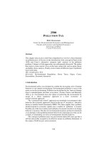
in Table 2.1. As an example of how such a table can be used,

suppose that a study area is divided into 116 quadrats as shown in
Figure 2.1, and it is desirable to select a simple random sample of ten
of these quadrats without replacement. To do this, first start at an
arbitrary place in the table such as the beginning of row five. The first
three digits in each block of five digits can then be considered, to give
the series 698, 419, 008, 127, 106, 605, 843, 378, 462, 953, 745, and
so on. The first ten different numbers between 1 and 116 then give a
simple random sample of quadrats: 8, 106, and so on. For selecting
large samples essentially the same process can be carried out on a
computer using pseudo-random numbers in a spreadsheet, for
example.
© 2001 by Chapman & Hall/CRC
Table 2.1 A random number table with each digit chosen such that
0, 1, , 9 were equally likely to occur. The grouping into groups of
four digits is arbitrary so that, for example, to select numbers from 0
to 99999 the digits can be considered five at a time
1252 9045 1286 2235 6289 5542 2965 1219 7088 1533
9135 3824 8483 1617 0990 4547 9454 9266 9223 9662
8377 5968 0088 9813 4019 1597 2294 8177 5720 8526
3789 9509 1107 7492 7178 7485 6866 0353 8133 7247
6988 4191 0083 1273 1061 6058 8433 3782 4627 9535
7458 7394 0804 6410 7771 9514 1689 2248 7654 1608
2136 8184 0033 1742 9116 6480 4081 6121 9399 2601
5693 3627 8980 2877 6078 0993 6817 7790 4589 8833
1813 0018 9270 2802 2245 8313 7113 2074 1510 1802
9787 7735 0752 3671 2519 1063 5471 7114 3477 7203
7379 6355 4738 8695 6987 9312 5261 3915 4060 5020
8763 8141 4588 0345 6854 4575 5940 1427 8757 5221
6605 3563 6829 2171 8121 5723 3901 0456 8691 9649
8154 6617 3825 2320 0476 4355 7690 9987 2757 3871

5855 0345 0029 6323 0493 8556 6810 7981 8007 3433
7172 6273 6400 7392 4880 2917 9748 6690 0147 6744
7780 3051 6052 6389 0957 7744 5265 7623 5189 0917
7289 8817 9973 7058 2621 7637 1791 1904 8467 0318
9133 5493 2280 9064 6427 2426 9685 3109 8222 0136
1035 4738 9748 6313 1589 0097 7292 6264 7563 2146
5482 8213 2366 1834 9971 2467 5843 1570 5818 4827
7947 2968 3840 9873 0330 1909 4348 4157 6470 5028
6426 2413 9559 2008 7485 0321 5106 0967 6471 5151
8382 7446 9142 2006 4643 8984 6677 8596 7477 3682
1948 6713 2204 9931 8202 9055 0820 6296 6570 0438
3250 5110 7397 3638 1794 2059 2771 4461 2018 4981
8445 1259 5679 4109 4010 2484 1495 3704 8936 1270
1933 6213 9774 1158 1659 6400 8525 6531 4712 6738
7368 9021 1251 3162 0646 2380 1446 2573 5018 1051
9772 1664 6687 4493 1932 6164 5882 0672 8492 1277
0868 9041 0735 1319 9096 6458 1659 1224 2968 9657
3658 6429 1186 0768 0484 1996 0338 4044 8415 1906
3117 6575 1925 6232 3495 4706 3533 7630 5570 9400
7572 1054 6902 2256 0003 2189 1569 1272 2592 0912
3526 1092 4235 0755 3173 1446 6311 3243 7053 7094
2597 8181 8560 6492 1451 1325 7247 1535 8773 0009
4666 0581 2433 9756 6818 1746 1273 1105 1919 0986
5905 5680 2503 0569 1642 3789 8234 4337 2705 6416
3890 0286 9414 9485 6629 4167 2517 9717 2582 8480
3891 5768 9601 3765 9627 6064 7097 2654 2456 3028
© 2001 by Chapman & Hall/CRC
Figure 2.1 A study area divided into 116 square quadrats to be used as
sample units.
2.3 Estimation of Population Means

Assume that a simple random sample of size n is selected without
replacement from a population of N units, and that the variable of
interest has values y
1
, y
2
, ,y
n
, for the sampled units. Then the
sample mean is
n
y
= 3 y
i
/ n, (2.1)
i = 1
the sample variance is
n
s² = { 3 (y
i
- y)²}/(n - 1), (2.2)
i =1
and the sample standard deviation is s, the square root of the
variance. Equations (2.1) and (2.2) are the same as equations (A1)
and (A2), respectively, in Appendix A except that the variable being
© 2001 by Chapman & Hall/CRC
considered is now labelled y instead of x. Another quantity that is
sometimes of interest is the sample coefficient of variation is
CV(y) = s/y
. (2.3)

These values that are calculated from samples are often referred
to as sample statistics. The corresponding population values are the
population mean µ, the population variance F
2
, the population
standard deviation F, and the population coefficient of variation F/µ.
These are often referred to as population parameters, and they are
obtained by applying equations (2.1) to (2.3) to the full set of N units
in the population. For example, µ is the mean of the observations on
all of the N units.
The sample mean is an estimator of the population mean µ. The
difference y
- µ is then the sampling error in the mean. This error will
vary from sample to sample if the sampling process is repeated, and
it can be shown theoretically that if this is done a large number of
times then the error will average out to zero. For this reason the
sample mean is said to be an unbiased estimator of the population
mean.
It can also be shown theoretically that the distribution of y
that is
obtained by repeating the process of simple random sampling without
replacement has the variance
Var(y
) = (F²/n)(1 - n/N). (2.4)
The factor {1 - n/N} is called the finite population correction because
it makes an allowance for the size of the sample relative to the size of
the population. The square root of Var(y
) is commonly called the
standard error of the sample mean. It will be denoted here by SE(y
)

= %Var(y
).
Because the population variance F
2
will not usually be known it
must usually be estimated by the sample variance s
2
for use in
equation (2.4). The resulting estimate of the variance of the sample
mean is then
Vâr(y
) = {s²/n}{1 - n/N}. (2.5)
The square root of this quantity is the estimated standard error of the
mean
© 2001 by Chapman & Hall/CRC
SÊ(y) = %[{s²/n}{1 - n/N}. (2.6)
The 'caps' on Vâr(y
) and SÊ(y) are used here to indicate estimated
values, which is a common convention in statistics.
The terms 'standard error of the mean' and 'standard deviation' are
often confused. What must be remembered is that the standard error
of the mean is just the standard deviation of the mean rather than the
standard deviation of individual observations. More generally, the
term 'standard error' is used to describe the standard deviation of any
sample statistic that is used to estimate a population parameter.
The accuracy of a sample mean for estimating the population
mean is often represented by a 100(1-")% confidence interval for the
population mean of the form
y
± z

"/2
SÊ(y), (2.7)
where z
"/2
refers to the value that is exceeded with probability "/2 for
the standard normal distribution, which can be determined using Table
B1 if necessary. This is an approximate confidence interval for
samples from any distribution, based on the result that sample means
tend to be normally distributed even when the distribution being
sampled is not. The interval is valid providing that the sample size is
larger than about 25 and the distribution being sampled is not very
extreme in the sense of having many tied values or a small proportion
of very large or very small values.
Commonly used confidence intervals are
y
± 1.64 SÊ(y) (90% confidence),
y
± 1.96 SÊ(y) (95% confidence), and
y
± 2.58 SÊ(y) (99% confidence).
Often a 95% confidence interval is taken as y
± 2 SÊ(y) on the
grounds of simplicity, and because it makes some allowance for the
fact that the standard error is only an estimated value.
The concept of a confidence interval is discussed in Section A5 of
Appendix A. A 90% confidence interval is, for example, an interval
within which the population mean will lie with probability 0.9. Put
another way, if many such confidence intervals are calculated, then
about 90% of these intervals will actually contain the population mean.
For samples that are smaller than 25 it is better to replace the

confidence interval (2.7) with
y
± t
"/2,n-1
SÊ(y), (2.8)
© 2001 by Chapman & Hall/CRC
where t
"/2,n-1
is the value that is exceeded with probability "/2 for the
t-distribution with n-1 degrees of freedom. This is the interval that is
justified in Section A5 of Appendix A samples from a normal
distribution, except that the standard error used in that case was just
s/%n because a finite population correction was not involved. The use
of the interval (2.8) requires the assumption that the variable being
measured is approximately normally distributed in the population
being sampled. It may not be satisfactory for samples from very non-
symmetric distributions.
Example 2.1 Soil Percentage in the Corozal District of Belize
As part of a study of prehistoric land use in the Corozal District of
Belize in Central America the area was divided into 151 plots of land
with sides 2.5 by 2.5 km (Green, 1973). A simple random sample of
40 of these plots was selected without replacement, and provided the
percentages of soils with constant lime enrichment that are shown in
Table 2.2. This example considers the use of these data to estimate
the average value of the measured variable (Y) for the entire area.
Table 2.2 Values for the percentage of soils with constant lime
enrichment for 40 plots of land of size 2.5 by 2.5 km chosen by
simple random sampling without replacement from 151 plots
comprising the Corozal District of Belize in Central America
100 10 100 10 20 40 75 0 60 0

40 40 5 100 60 10 60 50 100 60
20 40 20 30 20 30 90 10 90 40
50 70 30 30 15 50 30 30 0 60
The mean percentage for the sampled plots is 42.38, and the
standard deviation is 30.40. The estimated standard error of the
mean is then found from equation (2.6) to be
SÊ(y
) = %[{30.40²/40}{1 - 40/151}] = 4.12.
Approximate 95% confidence limits for the population mean
percentage are then found from equation (2.7) to be 42.38 ±
1.96x4.12, or 34.3 to 50.5.
© 2001 by Chapman & Hall/CRC
In fact, Green (1973) provides the data for all 151 plots in his
paper. The population mean percentage of soils with constant lime
enrichment is therefore known to be 47.7%. This is well within the
confidence limits, so the estimation procedure has been effective.
Note that the plot size used to define sample units in this example
could have been different. A larger size would have led to a
population with fewer sample units while a smaller size would have led
to more sample units. The population mean, which is just the
percentage of soils with constant lime enrichment in the entire study
area, would be unchanged.
2.4 Estimation of Population Totals
In many situations there is more interest in the total of all values in a
population, rather than the mean per sample unit. For example, the
total area damaged by an oil spill is likely to be of more concern than
the average area damaged on sample units. It turns out that the
estimation of a population total is straightforward providing that the
population size N is known, and an estimate of the population mean
is available. It is obvious, for example, that if a population consists of

500 plots of land, with an estimated mean amount of oil spill damage
of 15 square metres, then it is estimated that the total amount of
damage for the whole population is 500 x 15 = 7500 square metres.
The general equation relating the population total T
y
to the
population mean µ for a variable Y is T
y
= Nµ, where N is the
population size. The obvious estimator of the total based on a sample
mean y
is therefore
t
y
= Ny. (2.9)
The sampling variance of this estimator is
Var(t
y
) = N² Var(y), (2.10)
and its standard error (i.e., standard deviation) is
SE(t
y
) = N SE(y). (2.11)
Estimates of the variance and standard error are
Vâr(t
y
) = N² Vâr(y), (2.12)
and
© 2001 by Chapman & Hall/CRC
SÊ(t

y
) = N SÊ(y). (2.13)
In addition, an approximate 100(1-")% confidence interval for the
true population total can also be calculated in essentially the same
manner as described in the previous section for finding a confidence
interval for the population mean. Thus the limits are
t
y
± z
"/2
SÊ(t
y
). (2.14)
2.5 Estimation of Proportions
In discussing the estimation of population proportions it is important
to distinguish between proportions measured on sample units and
proportions of sample units. Proportions measured on sample units,
such as the proportions of the units covered by a certain type of
vegetation, can be treated like any other variables measured on the
units. In particular, the theory for the estimation of the mean of a
simple random sample that is covered in Section 2.3 applies for the
estimation of the mean proportion. Indeed, Example 2.1 was of
exactly this type except that the measurements on the sample units
were percentages rather than proportions (i.e., proportions multiplied
by 100). Proportions of sample units are different because the interest
is in which units are of a particular type. An example of this situation
is where the sample units are blocks of land and it is required to
estimate the proportion of all the blocks that show evidence of
damage from pollution. In this section only the estimation of
proportions of sample units is considered.

Suppose that a simple random sample of size n, selected without
replacement from a population of size N, contains r units with some
characteristic of interest. Then the sample proportion is pˆ = r/n, and
it can be shown that this has a sampling variance of
Var(pˆ) = {p(1 - p)/n}{1 - n/N}, (2.15)
and a standard error of SE(pˆ) = %Var(pˆ). These results are the same
as those obtained from assuming that r has a binomial distribution
(see Appendix Section A2), but with a finite population correction.
Estimated values for the variance and standard error can be
obtained by replacing the population proportion in equation (2.15) with
the sample proportion pˆ. Thus the estimated variance is
Vâr(pˆ) = [{pˆ(1 - pˆ)/n}{1 - n/N}], (2.16)
© 2001 by Chapman & Hall/CRC
and the estimated standard error is SÊ(pˆ) = %Vâr(pˆ). This creates
little error in estimating the variance and standard error unless the
sample size is quite small (say less than 20).
Using the estimated standard error, an approximate 100(1- ")%
confidence interval for the true proportion is
pˆ ± z
"/2
SÊ(pˆ), (2.17)
where, as before, z
"/2
is the value from the standard normal
distribution that is exceeded with probability "/2.
The confidence limits produced by equation (2.17) are based on
the assumption that the sample proportion is approximately normally
distributed, which it will be if np(1-p) $ 5 and the sample size is fairly
small in comparison to the population size. If this is not the case, then
alternative methods for calculating confidence limits should be used

(Cochran, 1977, Section 3.6).
Example 2.2 PCB Concentrations in Surface Soil Samples
As an example of the estimation of a population proportion, consider
some data provided by Gore and Patil (1994) on polychlorinated
biphenyl (PCB) concentrations in parts per million (ppm) at the
Armagh compressor station in West Wheatfield Township, along the
gas pipeline of the Texas Eastern Pipeline Gas Company in
Pennsylvania, USA. The cleanup criterion for PCB in this situation for
a surface soil sample is an average PCB concentration of 5 ppm in
soils between the surface and six inches in depth.
In order to study the PCB concentrations at the site, grids were set
surrounding four potential sources of the chemical, with 25 feet
separating the grid lines for the rows and columns. Samples were
then taken at 358 of the points where the row and column grid lines
intersected. Gore and Patil give the PCB concentrations at all of
these points. However, here the estimation of the proportion of the N
= 358 points at which the PCB concentration exceeds 5 ppm will be
considered, based on a random sample of n = 100 of the points,
selected without replacement.
The PCB values for the sample of 50 points are shown in Table
2.3. Of these, 31 exceed 5 ppm so that the estimate of the proportion
of exceedances for all 358 points is pˆ = 31/50 = 0.62. The estimated
variance associated with this proportion is then found from equation
(2.16) to be
© 2001 by Chapman & Hall/CRC
Vâr(pˆ) = {0.62 x 0.38/50}(1 - 50/358) = 0.0041.
Thus SÊ(pˆ) = 0.064, and the approximate confidence interval for the
proportion for all points, calculated from equation (2.17), is 0.495 to
0.745.
Table 2.3 PCB concentrations in parts per million at 50 sample points

from the Armagh compressor station
5.1 49.0 36.0 34.0 5.4 38.0 1000.0 2.1 9.4 7.5
1.3 140.0 1.3 75.0 0.0 72.0 0.0 0.0 14.0 1.6
7.5 18.0 11.0 0.0 20.0 1.1 7.7 7.5 1.1 4.2
20.0 44.0 0.0 35.0 2.5 17.0 46.0 2.2 15.0 0.0
22.0 3.0 38.0 1880.0 7.4 26.0 2.9 5.0 33.0 2.8
2.6 Sampling and Non-Sampling Errors
Four sources of error may affect the estimation of population
parameters from samples:
Sampling errors are due to the variability between sample units
and the random selection of units included in a sample.
Measurement errors are due to the lack of uniformity in the manner
in which a study is conducted, and inconsistencies in the
measurement methods used.
Missing data are due to the failure to measure some units in the
sample.
Errors of various types may be introduced in coding, tabulating,
typing and editing data.
The first of these errors is allowed for in the usual equations for
variances. Also, random measurement errors from a distribution with
a mean of zero will just tend to inflate sample variances, and will
therefore be accounted for along with the sampling errors. Therefore,
the main concerns with sampling should be potential bias due to
measurement errors that tend to be in one direction, missing data
values that tend to be different from the known values, and errors
introduced while processing data.
© 2001 by Chapman & Hall/CRC
The last three types of error are sometimes called non-sampling
errors. It is very important to ensure that these errors are minimal,
and to appreciate that unless care is taken they may swamp the

sampling errors that are reflected in variance calculations. This has
been well recognized by environmental scientists in the last 15 years
or so, with much attention given to the development of appropriate
procedures for quality assurance and quality control (QA/QC). These
matters are discussed by Keith (1991, 1996) and Liabastre et al.
(1992), and are also a key element in the data quality objectives
(DQO) process that is discussed in Section 2.15.
2.7 Stratified Random Sampling
A valid criticism of simple random sampling is that it leaves too much
to chance, so that the number of sampled units in different parts of the
population may not match the distribution in the population. One way
to overcome this problem while still keeping the advantages of random
sampling is to use stratified random sampling. This involves dividing
the units in the population into non-overlapping strata, and selecting
an independent simple random sample from each of these strata.
Often there is little to lose by using this more complicated type of
sampling but there are some potential gains. First, if the individuals
within strata are more similar than individuals in general, then the
estimate of the overall population mean will have a smaller standard
error than can be obtained with the same simple random sample size.
Second, there may be value in having separate estimates of
population parameters for the different strata. Third, stratification
makes it possible to sample different parts of a population in different
ways, which may make some cost savings possible.
However, stratification can also cause problems that are best
avoided if possible. This was the case with two of the Exxon Valdez
studies that were discussed in Example 1.1. Exxon's Shoreline
Ecology Program and the Oil Spill Trustees' Coastal Habitat Injury
Assessment were both upset to some extent by an initial
misclassification of units to strata which meant that the final samples

within the strata were not simple random samples. The outcome was
that the results of these studies either require a rather complicated
analysis or are susceptible to being discredited. The first problem that
can occur is therefore that the stratification used may end up being
inappropriate.
© 2001 by Chapman & Hall/CRC
Another potential problem with using stratification is that after the
data are collected using one form of stratification there is interest in
analysing the results using a different stratification that was not
foreseen in advance, or using an analysis that is different from the
original one proposed. Because of the many different groups
interested in environmental matters from different points of view this
is always a possibility, and it led Overton and Stehman (1995) to
argue strongly in favour of using simple sampling designs with limited
or no stratification.
If stratification is to be employed, then generally this should be
based on obvious considerations such as spatial location, areas within
which the population is expected to be uniform, and the size of
sampling units. For example, in sampling vegetation over a large area
it is natural to take a map and partition the area into a few apparently
homogeneous strata based on factors such as altitude and vegetation
type. Usually the choice of how to stratify is just a question of
common sense.
Assume that K strata have been chosen, with the ith of these
having size N
i
and the total population size being 3N
i
= N. Then if a
random sample with size n

i
is taken from the ith stratum the sample
mean y
i
will be an unbiased estimate of the true stratum mean µ
i
, with
estimated variance
Vâr(y
i
)=(s
i
2
/n
i
)(1 - n
i
/N
i
), (2.18)
where s
i
is the sample standard deviation within the stratum. These
results follow by simply applying the results discussed earlier for
simple random sampling to the ith stratum only.
In terms of the true strata means, the overall population mean is
the weighted average
K
µ = 3 N
i

µ
i
/N, (2.19)
i = 1
and the corresponding sample estimate is


K
y
s
= 3 N
i
y
i
/N, (2.20)


i = 1
with estimated variance
© 2001 by Chapman & Hall/CRC


K
Vâr(y
s
) = 3 (N
i
/N)² Vâr(y
i
)

i = 1
K
= 3 (N
i
/N)²(s
i
2
/n
i
)(1 - n
i
/N
i
). (2.21)
i = 1
The estimated standard error of y
s
is SÊ(y
s
), the square root of the
estimated variance, and an approximate 100(1-")% confidence
interval for the population mean is given by
y
s
± z
"/2
SÊ(y
s

), (2.22)
where z
"/2
is the value exceeded with probability "/2 for the standard
normal distribution.
If the population total is of interest, then this can be estimated by
t
s
= Ny
s
(2.23)
with estimated standard error
SÊ(t
s
) = N SÊ(y
s
). (2.24)
Again, an approximate 100(1-")% confidence interval takes the form
t
s
± z
"/2
SÊ(t
s
). (2.25)
Equations are available for estimating a population proportion from
a stratified sample (Scheaffer et al., 1990, Section 5.6). However, if
an indicator variable Y is defined which takes the value one if a
sample unit has the property of interest, and zero otherwise, then the
mean of Y in the population is equal to the proportion of the sample

units in the population that have the property. Therefore, the
population proportion of units with the property can be estimated by
applying equation (2.20) with the indicator variable, together with the
equations for the variance and approximate confidence limits.
When a stratified sample of points in a spatial region is carried out
it often will be the case that there are an unlimited number of sample
points that can be taken from any of the strata, so that N
i
and N are
infinite. Equation (2.20) can then be modified to
© 2001 by Chapman & Hall/CRC
K
y
s
= 3 w
i
y
i
, (2.26)
i = 1
where w
i
, the proportion of the total study area within the ith stratum,
replaces N
i
/N. Similarly, equation (2.21) changes to
K
Vâr(y
s
) = 3 w

i
² s
i
2
/n
i
. (2.27)


i = 1
Equations (2.22) to (2.25) remain unchanged.
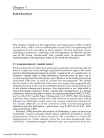
Example 2.3 Bracken Density in Otago
As part of an ongoing study of the distribution of scrub weeds in New
Zealand, data were obtained on the density of bracken on one hectare
(100m by 100m) pixels along a transect 90km long and 3km wide
running from Balclutha to Katiki Point on the South Island of New
Zealand, as shown in Figure 2.2 (Gonzalez and Benwell, 1994). This
example involves a comparison between estimating the density (the
percentage of the land in the transect covered with bracken) using (i)
a simple random sample of 400 pixels, and (ii) using a stratified
random sample with five strata and the same total sample size.
There are altogether 27,000 pixels in the entire transect, most of
which contain no bracken. The simple random sample of 400 pixels
was found to contain 377 with no bracken, 14 with 5% bracken, 6 with
15% bracken, and 3 with 30% bracken. The sample mean is therefore
y
= 0.625%, the sample standard deviation is s = 3.261, and the
estimated standard error of the mean is
SÊ(y
s

) = (3.261/%400)(1 - 400/27000) = 0.162.
The approximate 95% confidence limits for the true population mean
density is therefore 0.625 ± 1.96 x 0.162, or 0.31 to 0.94%.
The strata for stratified sampling were five stretches of the transect,
each about 18km long, and each containing 5400 pixels. The sample
results and some of the calculations for this sample are shown in
Table 2.4. The estimated population mean density from equation
(2.19) is 0.613%, with an estimated variance of 0.0208 from equation
(2.21). The estimated standard error is therefore %0.0208 = 0.144,
and an approximate 95% confidence limits for the true population
mean density is 0.613 ± 1.96 x 0.144, or 0.33 to 0.90%.
© 2001 by Chapman & Hall/CRC
In a situation being considered there might be some interest in
estimating the area in the study region covered by bracken. The total
area is 27,000 hectares. Therefore the estimate from simple random
sampling is 27,000 x 0.00625 = 168.8 hectares, with an estimated
standard error of 27,000 x 0.00162 = 43.7 hectares, expressing the
estimated percentage cover as a proportion. The approximate 95%
confidence limits are 27,000 x 0.0031 = 83.7 to 27,000 x 0.0094 =
253.8 hectares. Similar calculations with the results of the stratified
sample give an estimated coverage of 165.5 hectares, with a standard
error of 38.9 hectares, and approximate 95% confidence limits of 89.1
to 243.0 hectares.
In this example the advantage of using stratified sampling instead
of simple random sampling has not been great. The estimates of the
mean bracken density are quite similar and the standard error from
the stratified sample (0.144) is not much smaller than that for simple
random sampling (0.162). Of course, if it had been known in advance
that no bracken would be recorded in stratum 5, then the sample units
in that stratum could have been allocated to the other strata, leading

to some further reduction in the standard error. Methods for deciding
on sample sizes for stratified and other sampling methods are
discussed further in Section 2.13.
2.8 Post-Stratification
At times there may be value in analysing a simple random sample as
if it were obtained by stratified random sampling. That is to say, a
simple random sample is taken and the units are then placed into
strata, possibly based on information obtained at the time of sampling.
The sample is then analysed as if it were a stratified random sample
in the first place, using the equations given in the previous section.
This procedure is called post-stratification. It requires that the strata
sizes N
i
are known so that equations (2.20) and (2.21) can be used.
A simple random sample is expected to place sample units in
different strata according to the size of those strata. Therefore, post-
stratification should be quite similar to stratified sampling with
proportional allocation, providing that the total sample size is
reasonably large. It therefore has some considerable potential merit
as a method that permits the method of stratification to be changed
after a sample has been selected. This may be particularly valuable
in situations where the data may be used for a variety of purposes,
some of which are not known at the time of sampling.
© 2001 by Chapman & Hall/CRC
Figure 2.2 A transect about 90km long and 3km wide along which bracken
has been sampled in the South Island of New Zealand.
© 2001 by Chapman & Hall/CRC
Table 2.4 The results of stratified random sampling for estimating the
density of bracken along a transect in the South Island of New
Zealand

Stratum
Case 1 2 3 4 5
1 0 0 15 5 0 0 0 0 0 0
2 0 0 0 0 0 0 0 0 0 0
3 0 0 0 0 0 0 0 0 0 0
4 0 0 0 0 0 0 0 0 0 0
5 0 0 15 0 5 0 0 0 0 0
6 0 0 0 0 0 0 0 0 0 0
7 0 0 0 5 0 5 0 5 0 0
8 0 0 0 0 0 0 0 0 0 0
9 0 0 0 0 0 0 0 0 0 0
10 0 0 0 0 0 0 0 0 0 0
11 0 0 0 0 0 0 0 0 0 0
12 0 0 0 0 0 0 0 0 0 0
13 0 0 0 0 0 0 0 0 0 0
14 0 0 5 0 0 0 0 30 0 0
15 0 0 0 15 15 0 0 0 0 0
16 0 0 5 0 0 30 0 0 0 0
17 5 0 0 0 0 0 0 0 0 0
18 0 0 15 0 0 0 0 0 0 0
19 0 0 0 0 0 5 0 0 0 0
20 0 0 0 0 0 0 0 0 0 0
21 0 0 0 0 0 0 0 0 0 0
22 0 0 0 0 0 0 0 0 0 0
23 0 0 5 0 0 0 0 0 0 0
24 0 0 0 0 0 0 0 0 0 0
25 0 5 5 5 0 0 0 0 0 0
26 0 0 0 0 0 0 0 0 0 0
27 0 0 0 0 0 5 0 0 0 0
28 0 0 0 0 0 0 0 0 0 0

29 0 0 0 0 0 0 0 0 0 0
30 0 0 5 5 0 0 0 0 0 0
31 0 0 0 0 0 0 0 0 0 0
32 0 0 15 5 0 0 0 0 0 0
33 0 0 0 0 0 0 0 0 0 0
34 0 0 0 0 0 0 0 0 0 0
35 0 0 0 0 0 0 0 0 0 0
36 0 0 0 0 0 0 0 0 0 0
37 0 0 0 0 0 0 0 0 0 0
38 0 0 0 0 0 0 0 0 0 0
39 0 0 0 0 0 0 0 0 0 0
40 0 5 5 0 0 0 0 0 0 0
Mean 0.1875 1.625 0.8125 0.4375 0.000
SD 0.956 3.879 3.852 3.393 0.000 Total
n 80 80 80 80 80 400
N 5400 5400 5400 5400 5400 27000
Contributions to the sum in equation (2.19) for the estimated mean
0.0375 0.3250 0.1625 0.0875 0.0000 0.6125
Contributions to the sum in equation (2.21) for the estimated variance
0.0005 0.0074 0.0073 0.0057 0.0000 0.0208
© 2001 by Chapman & Hall/CRC
2.9 Systematic Sampling
Systematic sampling is often used as an alternative to simple random
sampling or stratified random sampling for two reasons. First, the
process of selecting sample units is simpler for systematic sampling.
Second, under certain circumstances estimates can be expected to
be more precise for systematic sampling because the population is
covered more evenly.
The basic idea with systematic sampling is to take every kth item
in a list, or to sample points that are regularly placed in space. As an

example, consider the situation that is shown in Figure 2.3. The top
part of the figure shows the positions of 12 randomly placed sample
points in a rectangular study area. The middle part shows a stratified
sample where the study region is divided into four equal sized strata,
and three sample points are placed randomly within each. The lower
part of the figure shows a systematic sample where the study area is
divided into 12 equal sized quadrats each of which contains a point at
the same randomly located position within the quadrat. Quite clearly,
stratified sampling has produced better control than random sampling
in terms of the way that the sample points cover the region, but not as
much control as systematic sampling.
It is common to analyse a systematic sample as if it were a simple
random sample. In particular, population means, totals and
proportions are estimated using the equations in Sections 2.3 to 2.5,
including the estimation of standard errors and the determination of
confidence limits. The assumption is then made that because of the
way that the systematic sample covers the population this will, if
anything, result in standard errors that tend to be somewhat too large
and confidence limits that tend to be somewhat too wide. That is to
say, the assessment of the level of sampling errors is assumed to be
conservative.
The only time that this procedure is liable to give a misleading
impression about the true level of sampling errors is when the
population being sampled has some cyclic variation in observations
so that the regularly spaced observations that are selected tend to all
be either higher or lower than the population mean. Therefore, if there
is a suspicion that regularly spaced sample points may follow some
pattern in the population values, then systematic sampling should be
avoided. Simple random sampling and stratified random sampling are
not affected by any patterns in the population, and it is therefore safer

to use them when patterns may be present.
© 2001 by Chapman & Hall/CRC
Figure 2.3 Comparison of simple random sampling, stratified random
sampling and systematic sampling for points in a rectangular study region.
The United States Environmental Protection Agency (1989a)
manual on statistical methods for evaluating the attainment of site
cleanup standards recommends two alternatives to treating a
systematic sample as a simple random sample for the purpose of
analysis. The first of these alternatives involves combining adjacent
points into strata, as indicated in Figure 2.4. The population mean
and standard error are then estimated using equations (2.26) and
(2.27). The assumption being made is that the sample within each of
the imposed strata is equivalent to a random sample. It is most
important that the strata are defined without taking any notice of the
© 2001 by Chapman & Hall/CRC
values of observations because otherwise bias will be introduced into
the variance calculation.
Figure 2.4 Grouping sample points from a systematic sample so that it can
be analysed as a stratified sample. The sample points ( •) are grouped here
into 10 strata each containing six points.
Figure 2.5 Defining a serpentine line connecting the points of a systematic
sample so that the sampling variance can be estimated using squared
differences between adjacent points on the line.
© 2001 by Chapman & Hall/CRC
If the number of sample points or the area is not the same within
each of the strata, then the estimated mean from equation (2.26) will
differ from the simple mean of all of the observations. This is to be
avoided because it will be an effect that is introduced by a more or
less arbitrary system of stratification. The estimated variance of the
mean from equation (2.27) will inevitably depend on the stratification

used and under some circumstances it may be necessary to show that
all reasonable stratifications give about the same result.
The second alternative to treating a systematic sample as a simple
random sample involves joining the sample points with a serpentine
line that joins neighbouring points and passes only once through each
point, as shown in Figure 2.5. Assuming that this has been done, and
that y
i
is the ith observation along the line, it is assumed that y
i-1
and
y
i
are both measures of the variable of interest in approximately the
same location. The difference squared (y
i
- y
i-1
)
2
is then an estimate
of twice the variance of what can be thought of as the local sampling
errors. With a systematic sample of size n there are n-1 such squared
differences, leading to a combined estimate of the variance of local
sampling errors of
n
s
L
2
= ½ 3 (y

i
- y
i-1
)
2
/(n-1). (2.28)
i = 2
On this basis the estimate of the standard error of the mean of the
systematic sample is
SÊ(y
) = s
L
/%n. (2.29)
No finite sampling correction is applied when estimating the standard
error on the presumption that the number of potential sampling points
in the study area is very large. Once the standard error is estimated
using equation (2.29) approximate confidence limits can be
determined using equation (2.7), and the population total can be
estimated using the methods described in Section 2.4. This approach
for assessing sampling errors was found to be as good or better than
seven alternatives from a study that was carried out by Wolter (1984).
Example 2.4 Total PCBs in Liverpool Bay Sediments
Camacho-Ibar and McEvoy (1996) describe a study that was aimed
at determining the concentrations of 55 polychlorinated biphenyl
(PCB) congeners in sediment samples from Liverpool Bay in the
© 2001 by Chapman & Hall/CRC
United Kingdom. For this purpose, the total PCB was defined as the
summation of the concentrations of all the identifiable individual
congeners that were present at detectable levels in each of 66 grab
samples taken between 14 and 16 September 1988. The values for

this variable and the approximate position of each sample are shown
in Figure 2.6. Although the sample locations were not systematically
placed over the bay, they are much more regularly spaced than can
be expected to occur with random sampling.
The mean and standard deviation of the 66 observations are y
=
3937.7 and s = 6646.5, in units of pg g
-1
(picograms per gram, i.e.,
parts per 10
12
). Therefore, if the sample is treated as being equivalent
to a simple random sample, then the estimated standard error is SÊ( y
)
= 6646.5/%66 = 818.1, and the approximate 95% confidence limits for
the mean over the sampled region are 3937.7 ± 1.96 x 818.1, or
2334.1 to 5541.2.
The second method for assessing the accuracy of the mean of a
systematic sample as described above entails dividing the samples
into strata. This division was done arbitrarily using 11 strata of six
observations each, as shown in Figure 2.7, and the calculations for
the resulting stratified sample are shown in Table 2.5. The estimated
mean level for total PCBs in the area is still 3937.7 pg g
-1
. However,
the standard error calculated from the stratification is 674.2, which is
lower than the value of 818.1 found by treating the data as coming
from a simple random sample. The approximate 95% confidence
limits from stratification are 3937.7 ± 1.96 x 674.2, or 2616.2 to
5259.1.

Finally, the standard error can be estimated using equations (2.28)
and (2.29), with the sample points in the order shown in Figure 2.7 but
with the closest points connected between the sets of six observations
that formed the strata before. This produces an estimated standard
deviation of s
L
= 5704.8 for small-scale sampling errors, and an
estimated standard error for the mean in the study area of SE
^
(y
) =
5704.8/%66 = 702.2. By this method the approximate 95% confidence
limits for the area mean are 3937.7 ± 1.96 x 702.2, or 2561.3 to
5314.0 pg g
-1
. This is quite close to what was obtained using the
stratification method.
© 2001 by Chapman & Hall/CRC
Figure 2.6 Concentration of total PCBs (pg g
-1
) in samples of sediment
taken from Liverpool Bay. Observations are shown at their approximate
position in the study area. The arrow points to the entrance to the River
Mersey.
2.10 Other Design Strategies
So far in this chapter the sample designs that have been considered
are simple random sampling, stratified random sampling, and
systematic sampling. There are also a number of other design
strategies that are sometimes used. Here some of the designs that
may be useful in environmental studies are just briefly mentioned. For

further details see Scheaffer et al. (1990), Thompson (1992), or some
other specialized text.
With cluster sampling, groups of sample units that are close in
some sense are randomly sampled together, and then all measured.
The idea is that this will reduce the cost of sampling each unit so that
more units can be measured than would be possible if they were all
sampled individually. This advantage is offset to some extent by the
tendency of sample units that are close together to have similar
measurements. Therefore, in general, a cluster sample of n units will
give estimates that are less precise than a simple random sample of
n units. Nevertheless, cluster sampling may give better value for
money than the sampling of individual units.
© 2001 by Chapman & Hall/CRC
Figure 2.7 Partitioning of samples in Liverpool bay into 11 strata consisting
of points that are connected by broken lines.
With multi-stage sampling, the sample units are regarded as falling
within a hierarchic structure. Random sampling is then conducted at
the various levels within this structure. For example, suppose that
there is interest in estimating the mean of some water quality variable
in the lakes in a very large area such as a whole country. The country
might then be divided into primary sampling units consisting of states
or provinces, each primary unit might then consist of a number of
counties, and each county might contain a certain number of lakes.
A three-stage sample of lakes could then be obtained by first
randomly selecting several primary sampling units, next randomly
selecting one or more counties (second-stage units) within each
sampled primary unit, and finally randomly selecting one or more
lakes (third-stage units) from each sampled county. This type of
sampling plan may be useful when a hierarchic structure already
exists, or when it is simply convenient to sample at two or more levels.

© 2001 by Chapman & Hall/CRC