Statistics for Environmental Science and Management - Chapter 8 ppsx

CHAPTER 8
Time Series Analysis
8.1 Introduction
Time series have had a role to play in several of the earlier chapters.
In particular, environmental monitoring (Chapter 5) usually involves
collecting observations over time at some fixed sites, so that there is a
time series for each of these sites, and the same is true for impact
assessment (Chapter 6). However, the emphasis in the present
chapter will be different, because the situations that will be considered
are where there is a single time series, which may be reasonably long
(say with 50 or more observations) and the primary concern will often
be to understand the structure of the series.
There are several reasons why a time series analysis may be
important. For example:
It gives a guide to the underlying mechanism that produces the
series.
It is sometimes necessary to decide whether a time series displays
a significant trend, possibly taking into account serial correlation
which, if present, can lead to the appearance of a trend in stretches
of a time series although in reality the long-run mean of the series
is constant.
A series shows seasonal variation through the year which needs to
be removed in order to display the true underlying trend.
The appropriate management action depends on the future values
of a series, so it is desirable to forecast these and understand the
likely size of differences between the forecast and true values.
There is a vast literature on the modelling of time series. It is not
possible to cover this in any detail here, so what is done is just to
provide an introduction to some of the more popular types of models,
and provide references to where more information can be found.
© 2001 by Chapman & Hall/CRC

8.2 Components of Time Series
To illustrate the types of time series that arise, some examples can be
considered. The first is Jones et al.'s (1998a,b) temperature
reconstructions for the northern and southern hemispheres, 1000 to
1991 AD. These two series were constructed using data on
temperature-sensitive proxy variables including tree rings, ice cores,
corals, and historic documents, from 17 sites worldwide. They are
plotted in Figure 8.1.
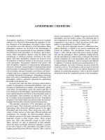
Figure 8.1 Average northern and southern hemisphere temperature series
1000 to 1991 AD calculated by Jones et al. (1998a,b) using data from
temperature-sensitive proxy variables at 17 sites worldwide. The heavy
horizontal lines on each plot are the overall mean temperatures.
The series are characterised by a considerable amount of year to
year variation, with excursions away from the overall mean for periods
up to about 100 years, with these excursions being more apparent in
the northern hemisphere series. The excursions are typical of the
behaviour of series with a fairly high level of serial correlation.
In view of the current interest in global warming it is interesting to
see that the northern hemisphere temperatures in the latter part of the
present century are warmer than the overall mean, but similar to those
seen in the latter part of the tenth century, although somewhat less
© 2001 by Chapman & Hall/CRC
variable. The recent pattern of warm southern hemisphere
temperatures is not seen earlier in the series.
A second example is a time series of the water temperature of a
stream in Dunedin, New Zealand, measured every month from January
1989 to December 1997. The series is plotted in Figure 8.2. In this
case, not surprisingly, there is a very strong seasonal component, with
the warmest temperatures in January to March, and the coldest
temperatures in about the middle of the year. There is no clear trend,

although the highest recorded temperature was in January 1989, and
the lowest was in August 1997.
Figure 8.2 Water temperatures measured on a stream in Dunedin, New
Zealand, at monthly intervals from January 1989 to December 1997. The
overall mean is the heavy horizontal line.
A third example is the estimated number of pairs of the sandwich
tern (Sterna sandvicenis) on Dutch Wadden Island, Griend, for the
years 1964 to 1995, as provided by Schipper and Meelis (1997). The
situation is that in the early 1960s the number of breeding pairs
decreased dramatically because of poisoning by chlorated
hydrocarbons. The discharge of these toxicants was stopped in 1964,
and estimates of breeding pairs were then made annually to see
whether numbers increased. Figure 8.3 shows the estimates obtained.
The time series in this case is characterised by an upward trend,
with substantial year to year variation around this trend. Another point
to note is that the year to year variation increased as the series
increased. This is an effect that is frequently observed in series with a
strong trend.
Finally, Figure 8.4 shows yearly sunspot numbers from 1700 to the
present (Sunspot Index Data Center, 1999). The most obvious
characteristic of this series is the cycle of about 11 years, although it is
© 2001 by Chapman & Hall/CRC
also apparent that the maximum sunspot number varies considerably
from cycle to cycle.
The examples demonstrate the types of components that may
appear in a time series. These are:
(a) a trend component, such that there is a long-term tendency for the
values in the series to increase or decrease (as for the sandwich
tern);
(b) a seasonal component for series with repeated measurements

within calendar years, such that observations at certain times of the
year tend to be higher or lower than those at certain other times of
the year (as for the water temperatures in Dunedin);
(c) a cyclic component that is not related to the seasons of the year (as
for sunspot numbers);
(d) a component of excursions above or below the long-term mean or
trend that is not associated with the calendar year (as for global
temperatures); and
(e) a random component affecting individual observations (as in all the
examples).
These components cannot necessarily be separated easily. For
example, it may be a question of definition as to whether the
component (d) is part of the trend in a series, or is a deviation from the
trend.
Figure 8.3 The estimated number of breeding sandwich tern pairs on the
Dutch Wadden Island, Griend, from 1964 to 1995.
© 2001 by Chapman & Hall/CRC
Figure 8.4 Yearly sunspot numbers since 1700 from the Sunspot Index Data
Center maintained by the Royal Observatory of Belgium.
8.3 Serial Correlation
Serial correlation coefficients measure the extent to which the
observations in a series separated by different time differences tend to
be similar. They are calculated in a similar way to the usual Pearson
correlation coefficient between two variables. Given data (x
1
,y
1
), (x
2
,y

2
),
, (x
n
,y
n
) on n pairs of observations for variables X and Y, the sample
Pearson correlation is calculated as
n n

n
r = 3 (x
i
- x)(y
i
- y) / %[ 3 (x
i
- x)
2
3 (y
i
- y)
2
], (8.1)
i = 1 i = 1 i = 1
where x
is the sample mean for X and y is the sample mean for Y.
Equation (8.1) can be applied directly to the values (x
1
,x

2
), (x
2
,x
3
), ,
(x
n-1
,x
n
) in a time series to estimate the serial correlation, r
1
, between
terms one time period apart. However, what is usually done is to
calculate this using a simpler equation, such as
n -1 n
r
1
= [ 3 (x
i
- x)(x
i+1
- x)/(n - 1)]/[ 3 (x
i
- x)
2
] / n], (8.2)
i = 1 i = 1
where x
is the mean of the whole series. Similarly, the correlation

between x
i
and x
i+k
can be estimated by
n - k n
r
k
= [ 3 (x
i
- x)(x
i+k
- x) / (n - k)] / [ 3 (x
i
- x)
2
/ n]. (8.3)
i = 1 i = 1
© 2001 by Chapman & Hall/CRC
This is sometimes called the autocorrelation at lag k.
There are some variations on equations (8.2) and (8.3) that are
sometimes used, and when using a computer program it may be
necessary to determine what is actually calculated. However, for long
time series the different varieties of equations give almost the same
values.
The correlogram, which is also called the autocorrelation function
(ACF), is a plot of the serial correlations r
k
against k. It is a useful
diagnostic tool for gaining some understanding of the type of series that

is being dealt with. A useful result in this respect is that if a series is not
too short (say n > 40) and consists of independent random values from
a single distribution (i.e., there is no autocorrelation), then the statistic
r
k
will approximately normally distributed with a mean of
E(r
k
) . -1/(n - 1), (8.4)
and a variance of
Var(r
k
) . 1/n. (8.5)
The significance of the sample serial correlation r
k
can therefore be
assessed by seeing whether it falls within the limits -1/(n - 1) ± 1.96/ %n.
If it is within these limits, then it is not significantly different from 0 at
about the 5% level.
Note that there is a multiple testing problem here because if r
1
to r
20
are all tested at the same time, for example, then one of these values
can be expected to be significant by chance (Section 4.9). This
suggests that the limits -1/(n - 1) ± 1.96/%n should be used only as a
guide to the importance of serial correlation, with the occasional value
outside the limits not being taken too seriously.
Figures 8.5 shows the correlograms for the global temperature time
series (Figure 8.1). It is interesting to see that these are quite different

for the northern and southern hemisphere temperatures. It appears
that for some reason the northern hemisphere temperatures are
significantly correlated even up to about 70 years apart in time.
However, the southern hemisphere temperatures show little correlation
after they are two years or more apart in time.
© 2001 by Chapman & Hall/CRC
Figure 8.5 Correlograms for northern and southern hemisphere
temperatures, 1000 to 1991 AD, with the broken horizontal lines indicating the
limits within which autocorrelations are expected to lie 95% of the time for
random series of this length.
Figure 8.6 shows the correlogram for the series of monthly
temperatures measured for a Dunedin stream (Figure 8.2). Here the
effect of seasonal variation is very apparent, with temperatures showing
high but decreasing correlations for 12, 24, 36 and 48 month time lags.
Figure 8.6 Correlogram for the series of monthly temperatures in a Dunedin
stream, with the broken horizontal lines indicating the limits on
autocorrelations expected for a random series of this length.
The time series of the estimated number of pairs of the sandwich
tern on Wadden Island displays increasing variation as the mean
increases (Figure 8.3). However, the variation is more constant if the
© 2001 by Chapman & Hall/CRC
logarithm to base 10 of the estimated number of pairs is considered
(Figure 8.7). The correlogram has therefore been calculated for the
logarithm series, and this is shown in Figure 8.8. Here the
autocorrelation is high for observations one year apart, decreases to
about -0.4 for observations 22 years apart, and then starts to increase
again. This pattern must be largely due to the trend in the series.
Figure 8.7 Logarithms (base 10) of the estimated number of pairs of the
sandwich tern at Wadden Island.
Figure 8.8 Correlogram for the series of logarithms of the number of pairs of

sandwich terns on Wadden Island, with the broken horizontal lines indicating
the limits on autocorrelations expected for a random series of this length.
Finally, the correlogram for the sunspot numbers series (Figure 8.4)
is shown in Figure 8.9. The 11 year cycle shows up very obviously with
high but decreasing correlations for 11, 22, 33 and 44 years. The
pattern is similar to what is obtained from the Dunedin stream
temperature series with a yearly cycle.
© 2001 by Chapman & Hall/CRC
If nothing else, these examples demonstrate how different types of
time series exhibit different patterns of structure.
Figure 8.9 Correlogram for the series of sunspot numbers, with the broken
horizontal lines indicating the limits on autocorrelations expected for a random
series of this length.
8.4 Tests for Randomness
A random time series is one which consists of independent values from
the same distribution. There is no serial correlation and this is the
simplest type of data that can occur.
There are a number of standard non-parametric tests for
randomness that are sometimes included in statistical packages. These
may be useful for a preliminary analysis of a time series to decide
whether it is necessary to do a more complicated analysis. They are
called 'non-parametric' because they are only based on the relative
magnitude of observations rather than assuming that these observations
come from any particular distribution.
One test is the runs above and below the median test. This involves
replacing each value in a series by 1 if it is greater than the median, and
0 if it is less than or equal to the median. The number of runs of the
same value is then determined, and compared with the distribution
expected if the zeros and ones are in a random order. For example,
consider the following series: 1 2 5 4 3 6 7 9 8. The median is 5, so that

the series of zeros and ones is 0 0 0 0 0 1 1 1 1. There are M = 2 runs,
so this is the test statistic. The trend in the initial series is reflected in M
being the smallest possible value. This then needs to be compared with
the distribution that is obtained if the zeros and ones are in a random
order.
© 2001 by Chapman & Hall/CRC
For short series (20 or fewer observations) the observed value of M
can be compared with the exact distribution when the null hypothesis is
true using tables provided by Swed and Eisenhart (1943), Siegel (1956),
or Madansky (1988), among others. For longer series this distribution
is approximately normal with mean
µ
M
= 2r(n - r)/n + 1, (8.6)
and variance
F
2
M
= 2r(n - r){2r(n - r) - n}/{n
2
(n - 1)}, (8.7)
where r is the number of zeros (Gibbons, 1986, p. 556). Hence
Z = (M - µ
M
)/F
M
can be tested for significance by comparison with the standard normal
distribution (possibly modified with the continuity correction described
below).
Another non-parametric test is the sign test. In this case the test

statistic is P, the number of positive signs for the differences x
2
- x
1
, x
3
-
x
2
, , x
n
- x
n-1
. If there are m differences after zeros have been
eliminated, then the distribution of P has mean
µ
P
= m/2, (8.8)
and variance
F
2
P
= m/12, (8.9)
for a random series (Gibbons, 1986, p. 558). The distribution
approaches a normal distribution for moderate length series (say 20
observations or more).
The runs up and down test is also based on the differences between
successive terms in the original series. The test statistic is R, the
observed number of 'runs' of positive or negative differences. For
example, in the case of the series 1 2 5 4 3 6 7 9 8 the signs of the

differences are + + - - + + + +, and R = 3. For a random series the
mean and variance of the number of runs are
µ
R
= (2m+1)/3, (8.10)
and
© 2001 by Chapman & Hall/CRC
F
2
R
= (16m-13)/90, (8.11)
where m is the number of differences (Gibbons, 1986, p. 557). A table
of the distribution is provided by Bradley (1968) among others, and C is
approximately normally distributed for longer series (20 or more
observations).
When using the normal distribution to determine significance levels
for these tests of randomness it is desirable to make a continuity
correction to allow for the fact that the test statistics are integers. For
example, suppose that there are M runs above and below the median,
which is less than the expected number µ
M
. Then the probability of a
value this far from µ
M
is twice the integral of the approximating normal
distribution from minus infinity to M + ½, providing that M + ½ is less
than µ
M
. The reason for taking the integral up to M + ½ rather than M is
to take into account the probability of getting exactly M runs, which is

approximated by the area from M - ½ to M + ½ under the normal
distribution. In a similar way, if M is greater than µ
M
then twice the area
from M - ½ to infinity is the probability of M being this far from µ
M
,
providing that M - ½ is greater than µ
M
. If µ
M
lies within the range from
M - ½ to M + ½, then the probability of being this far or further from µ
M
is exactly one.
Example 8.1 Minimum Temperatures in Uppsala, 1900 to 1981
To illustrate the tests for randomness just described, consider the data
in Table 8.1 for July minimum temperatures in Uppsala, Sweden, for the
years 1900 to 1981. This is part of a long series started by Anders
Celsius, the Professor of Astronomy at the University of Uppsala, who
started collecting daily measurements in the early part of the eighteenth
century. There are almost complete daily temperatures from the year
1739, although true daily minimums are only recorded from 1839 when
a maximum-minimum thermometer started to be used (Jandhyala et al.,
1999). Minimum temperatures in July are recorded by Jandhyala et al.
for the years 1774 to 1981, as read from a figure given by Leadbetter et
al. (1983), but for the purpose of this example only the last part of the
series is tested for randomness.
A plot of the series is shown in Figure 8.10. The temperatures were
low in the early part of the century, but then increased and became fairly

constant.
The number of runs above and below the median is M = 42. From
equations (8.6) and (8.7) the expected number of runs for a random
series is also µ
M
= 42.0, with standard deviation F
M
= 4.50. Clearly, this
is not a significant result. For the sign test, the number of positive
© 2001 by Chapman & Hall/CRC
differences is P = 44, out of m = 81 non-zero differences. From
equations (8.8) and (8.9) the mean and standard deviation for P for a
random series are µ
P
= 40.5 and F
P
= 2.6. With the continuity correction
described above, the significance can be determined by comparing Z =
(P- ½ - µ
P
)/F
P
= 1.15 with the standard normal distribution. The
probability of a value this far from zero is 0.25. Hence this gives little
evidence of non-randomness. Finally, the observed number of runs up
and down is R = 49. From equations (8.10) and (8.11) the mean and
standard deviation of R for a random series are µ
R
= 54.3 and F
R

= 3.8.
With the continuity correction the observed R corresponds to a score of
Z = -1.28 for comparing with the standard normal distribution. The
probability of a value this far from zero is 0.20, so this is another
insignificant result.
Table 8.1 Minimum July temperatures in Uppsala (EC) for the years 1900
to 1981 (Source: Jandhyala et al., 1999)
Year Temp Year Temp Year Temp Year Temp Year Temp
1900 5.5 1920 8.4 1940 11.0 1960 9.0 1980 9.0
1901 6.7 1921 9.7 1941 7.7 1961 9.9 1981 12.1
1902 4.0 1922 6.9 1942 9.2 1962 9.0
1903 7.9 1923 6.7 1943 6.6 1963 8.6
1904 6.3 1924 8.0 1944 7.1 1964 7.0
1905 9.0 1925 10.0 1945 8.2 1965 6.9
1906 6.2 1926 11.0 1946 10.4 1966 11.8
1907 7.2 1927 7.9 1947 10.8 1967 8.2
1908 2.1 1928 12.9 1948 10.2 1968 7.0
1909 4.9 1929 5.5 1949 9.8 1969 9.7
1910 6.6 1930 8.3 1950 7.3 1970 8.2
1911 6.3 1931 9.9 1951 8.0 1971 7.6
1912 6.5 1932 10.4 1952 6.4 1972 10.5
1913 8.7 1933 8.7 1953 9.7 1973 11.3
1914 10.2 1934 9.3 1954 11.0 1974 7.4
1915 10.8 1935 6.5 1955 10.7 1975 5.7
1916 9.7 1936 8.3 1956 9.4 1976 8.6
1917 7.7 1937 11.0 1957 8.1 1977 8.8
1918 4.4 1938 11.3 1958 8.2 1978 7.9
1919 9.0 1939 9.2 1959 7.4 1979 8.1
© 2001 by Chapman & Hall/CRC
Figure 8.10 Minimum July temperatures in Uppsala, Sweden, for the years

1900 to 1981.
None of the non-parametric tests for randomness give any evidence
against this hypothesis, even though it appears that the mean of the
series was lower in the early part of the century than it has been more
recently. This suggests that it is also worth looking at the correlogram,
which indicates some correlation in the series from one year to the next.
But even here the evidence for non-randomness is not very marked
(Figure 8.11). The question of whether the mean was constant for this
series is considered again in the next section.
Figure 8.11 Correlogram for the minimum July temperatures in Uppsala, with
the 95% limits on autocorrelations for a random series shown by the broken
horizontal lines.
© 2001 by Chapman & Hall/CRC
8.5 Detection of Change Points and Trends
Suppose that a variable is observed at a number of points of time, to
give a time series x
1
, x
2
, , x
n
. The change point problem is then to
detect a change in the mean of the series if this has occurred at an
unknown time between two of the observations. The problem is much
easier if the point where a change might have occurred is know, which
then requires what is sometimes called an intervention analysis.
A formal test for the existence of a change point seems to have first
been proposed by Page (1955) in the context of industrial process
control. Since that time a number of other approaches have been
developed, as reviewed by Jandhyala and MacNeill (1986), and

Jandhyala et al. (1999). Methods for detecting a change in the mean of
an industrial process through control charts and related techniques have
been considerably developed (Sections 5.7 and 5.8). Bayesian
methods have also been investigated (Carlin et al., 1992), and Sullivan
and Woodhall (1996) suggest a useful approach for examining data for
a change in the mean and/or the variance at an unknown time.
The main point to note about the change point problem is that it is
not valid to look at the time series, decide where a change point may
have occurred, and then test for a significant difference between the
means for the observations before and after the change. This is
because the maximum mean difference between two parts of the time
series may be quite large by chance alone and is liable to be statistically
significant if it is tested ignoring the way that it was selected. Some type
of allowance for multiple testing (Section 4.9) is therefore needed. See
the references given above for details of possible approaches.
A common problem with an environmental time series is the
detection of a monotonic trend. Complications include seasonality and
serial correlation in the observations. When considering this problem
it is most important to define the time scale that is of interest. As
pointed out by Loftis et al. (1991), in most analyses that have been
conducted in the past there has been an implicit assumption that what
is of interest is a trend over the time period for which data happen to be
available. For example, if 20 yearly results are known, then a 20 year
trend has implicitly been of interest. This then means that an increase
in the first ten years followed by a decrease in the last ten years to the
original level has been considered to give no overall trend, with the
intermediate changes possibly being thought of as due to serial
correlation. This is clearly not appropriate if systematic changes over
a five year period (say) are thought of by managers as being 'trend'.
When serial correlation is negligible, regression analysis provides a

very convenient framework for testing for trend. In simple cases, a
regression of the measured variable against time will suffice, with a test
© 2001 by Chapman & Hall/CRC
to see whether the coefficient of time is significantly different from zero.
In more complicated cases there may be a need to allow for seasonal
effects and the influence of one or more exogenous variables. Thus, for
example, if the dependent variable is measured monthly, then the type
of model that might be investigated is
Y
t
= ß
1
M
1 t
+ ß
2
M
2 t
+ + ß
12
M
12 t
+ "X
t
+ 2t + ,
t
, (8.12)
where Y
t
is the observation at time t, M

kt
is a month indicator that is 1
when the observation is for month k or is otherwise 0, X
t
is a relevant
covariate measured at time t, and ,
t
is a random error. Then the
parameters ß
1
to ß
12
allow for differences in Y values related to months
of the year, the parameter " allows for an effect of the covariate, and 2
is the change in Y per month after adjusting for any seasonal effects and
effects due to differences in X from month to month. There is no
separate constant term because this is incorporated by the allowance
for month effects. If the estimate of 2 obtained by fitting the regression
equation is significant, then this provides the evidence for a trend.
A small change can be made to the model in order to test for the
existence of seasonal effects. One of the month indicators (say the first
or last) can be omitted from the model and a constant term introduced.
A comparison between the fit of the model with just a constant and the
model with the constant and month indicators then shows whether the
mean value appears to vary from month to month.
If a regression equation such as the one above is fitted to data, then
a check for serial correlation in the error variable ,
ij
should always be
made. The usual method involves using the Durbin-Watson test (Durbin

and Watson, 1951), for which the test statistic is
n n
V = 3 (e
i
- e
i-1
) / 3 e
i
2
, (8.13)
i = 2 i = 1
where there are n observations altogether, and e
1
to e
n
are the
regression residuals in time order. The expected value of V is 2 when
there is no autocorrelation. Values less than 2 indicate a tendency for
observations that are close in time to be similar (positive
autocorrelation), and values greater than 2 indicate a tendency for close
observations to be different (negative autocorrelation).
Table B5 can be used to assess the significance of an observed
value of V for a two-sided test at the 5% level. The test is a little unusual
as there are values of V that are definitely not significant, values where
the significance is uncertain, and values that are definitely significant.
This is explained with the table. The Durbin-Watson test does assume
© 2001 by Chapman & Hall/CRC
that the regression residuals are normally distributed. It should
therefore be used with caution if this does not seem to be the case.
If autocorrelation seems to be present, then the regression model

can still be used. However, it should be fitted using a method that is
more appropriate than ordinary least-squares. Edwards and Coull
(1987), Judge et al. (1988, pp. 388-93 and 532-8), Neter et al. (1983,
Chapter 13) and Zetterqvist (1991) all describe how this can be done.
Some statistical packages provide one or more of these methods as
options. One simple approach is described in Section 8.6 below.
Actually, some researchers have tended to favour non-parametric
tests for trend because of the need to analyse large numbers of series
with a minimum amount of time devoted to considering the special
needs of each series. Thus transformations to normality, choosing
models, etc. are to be avoided if possible. The tests for randomness
that have been described in the previous section are possibilities in this
respect, with all of them being sensitive to trends to some extent.
However, the non-parametric methods that currently appear to be most
useful are the Mann-Kendall test, the seasonal Kendall test, and the
seasonal Kendall test with a correction for serial correlation (Taylor and
Loftis, 1989; Harcum et al., 1992).
The Mann-Kendall test is appropriate for data that do not display
seasonal variation, or for seasonally corrected data, with negligible
autocorrelation. For a series x
1
, x
2
, , x
n
the test statistic is the sum of
the signs of the differences between all pairwise observations,
n i - 1
S = 3 3 sign(x
i

- x
j
), (8.14)
i = 2 j = 1
where sign(z) is -1 for z < 0, 0 for z = 0, and +1 for z > 0. For a series
of values in a random order the expected value of S is zero and the
variance is
Var(S) = n(n - 1)(2n + 5)/18. (8.15)
To test whether S is significantly different from zero it is best to use a
special table if n is ten or less (Helsel and Hirsch, 1992, p. 469). For
larger values of n, Z
S
= S/%Var(S) can be compared with critical values
for the standard normal distribution.
To accommodate seasonality in the series being studied, Hirsch et
al. (1982) introduced the seasonal Kendall test. This involves
calculating the statistic S separately for each of the seasons of the year
(weeks, months, etc.) and uses the sum for an overall test. Thus if S
j
is
the value of S for season j, then on the null hypothesis of no trend S
T
=
© 2001 by Chapman & Hall/CRC
3S
j
has an expected value of 0 and a variance of Var(S
T
) = 3Var(S
j

).
The statistic Z
T
=S
T
/%Var(S
T
) can therefore be used for an overall test of
trend by comparing it with the standard normal distribution. Apparently
the normal approximation is good providing that the total series length
is 25 or more.
An assumption with the seasonal Kendall test is that the statistics for
the different seasons are independent. When this is not the case an
adjustment for serial correlation can be made when calculating Var( 3S
T
)
(Hirsch and Slack, 1984; Zetterqvist, 1991). An allowance for missing
data can also be made in this case.
Finally, an alternative approach for estimating the trend in a series
without assuming that it can be approximated by a particular parametric
function involves using a moving average type of approach. Computer
packages often offer this type of approach as an option, and more
details can be found in specialist texts on time series analysis (e.g.,
Chatfield, 1989, p. 13).
Example 8.2 Minimum Temperatures in Uppsala, Reconsidered
In Example 8.1 tests for randomness were applied to the data in Table
8.1 on minimum July temperatures in Uppsala for the years 1900 to
1981. None of the tests gave evidence for non-randomness, although
some suggestion of autocorrelation was found. The non-significant
results seem strange because the plot of the series (Figure 8.10) gives

an indication that the minimum temperatures tended to be low in the
early part of the century. In this example the series is therefore
reexamined, with evidence for changes in the mean level of the series
being specifically considered.
First, consider a regression model for the series, of the form
Y
t
= $
0
+ $
1
t + $
2
t
2
+ + $
p
t
p
+ ,
t
, (8.16)
where Y
t
is the minimum July temperature in year t, taking t = 1 for 1900
and t = 82 for 1981, and ,
t
is a random deviation from the value given
by the polynomial for the year t. Trying linear, quadratic, cubic and
quartic models gives the analysis of variance shown in Table 8.2. It is

found that the linear and quadratic terms are highly significant, the cubic
term is not significant at the 5% level, and the quartic term is not
significant at all. A quadratic model therefore seems appropriate.
© 2001 by Chapman & Hall/CRC
Table 8.2 Analysis of variance for polynomial trend models fitted to the
time series of minimum July temperatures in Uppsala
Source of
variation
Sum of
squares
Degrees
of freedom
Mean
square F-ratio
Significance
(p-value)
Time 31.64 1 31.64 10.14 0.002
Time
2
29.04 1 29.04 9.31 0.003
Time
3
9.49 1 9.49 3.04 0.085
Time
4
2.23 1 2.23 0.71 0.400
Error 240.11 77 3.12
Total 312.51 81
When a simple regression model like this is fitted to a time series it
is most important to check that the estimated residuals do not display

autocorrelation. The Durbin-Watson statistic of equation (8.13) is V =
1.69 for this example. With n = 82 observations and p = 2 regression
variables, Table B5 shows that to be definitely significant at the 5% level
on a two-sided test V would have to be less than about 1.52. Hence
there is little concern about autocorrelation for this example.
Figure 8.12 shows plots of the original series, the fitted quadratic
trend curve, and the standardized residuals (the differences between the
observed temperature and the fitted trend values divided by the
estimated residual standard deviation). The model appears to be a very
satisfactory description of the data, with the expected temperature
appearing to increase from 1900 to 1930 and then remain constant, or
even decline slightly. The residuals from the regression model are
approximately normally distributed, with almost all of the standardized
residuals in the range from -2 to +2.
© 2001 by Chapman & Hall/CRC
Figure 8.12 A quadratic trend fitted to the series of minimum July
temperatures in Uppsala (top graph), with the standardized residuals from the
fitted trend (lower graph).
The Mann-Kendall test using the statistic S calculated using equation
(8.14) also gives strong evidence of a trend in the mean of this series.
The observed value of S is 624, with a standard deviation of 249.7. The
Z-score for testing significance is therefore Z = 624/249.7 = 2.50, and
the probability of a value this far from zero is 0.012 for a random series.
See Smith (1993) for a discussion of other approaches for the
analysis of long-term weather data.
8.6 More Complicated Time Series Models
The internal structure of time series can mean that quite complicated
models are needed to describe the data. No attempt will be made here
to cover the huge literature on this topic. Instead, the most commonly
used types of models will be described, with some simple examples of

their use. For more information a specialist text such as that of Chatfield
(1989) should be consulted.
The possibility of allowing for autocorrelation with a regression model
was mentioned in the last section. Assuming the usual regression
situation where there are n values of a variable Y and corresponding
values for variables X
1
to X
p
, one simple approach that can be used is
as follows:
© 2001 by Chapman & Hall/CRC
(a) Fit the regression model
y
t
= $
0
+ $
1
x
1t
+ + $
p
x
pt
+ ,
t
,
in the usual way, where y
t

is the Y value at time t, for which the
values of X
1
to X
p
are x
1t
to x
pt
, respectively, and ,
t
is the error term.
Let the estimated equation be
y
^
= b
0
+ b
1
x
1t
+ + b
p
x
pt
,
with estimated regression residuals
e
t
= (y

t
- y
^

t
).
(b) Assume that the residuals in the original series are correlated
because they are related by an equation of the form
,
t
= ",
t-1
+ u
t
,
where " is a constant and u
t
is a random value from a normal
distribution with mean zero and a constant standard deviation. Then
it turns out that " can be estimated by "
^
, the first order serial
correlation for the estimated regression residuals.
(c) Note that from the original regression model
y
t
- "y
t-1
= $
0

(1 - ") + $
1
(x
1t
- "x
1t-1
) + + $
p
(x
pt
- "x
pt-1
) + ,
t
- ",
t-1
or
z
t
= ( + $
1
v
1t
+ + $
p
v
pt
+ u
t
,

where z
t
= y
t
- "y
t-1
, ( = $
0
(1 - "), and v
it
= x
it
- "x
it-1
, for i = 1, 2, , p.
This is now a regression model with independent errors, so that the
coefficients ( and $
1
to $
p
can be estimated by ordinary regression,
with all the usual tests of significance, etc. Of course, " is not
known. The approximate procedure actually used is therefore to
replace " with the estimate "
^
for the calculation of the z
t
and v
it
values.

These calculations can be done easily enough in most statistical
packages. A variation called the Cochran-Orcutt procedure involves
iterating using steps (b) and (c). What is then done is to recalculate the
regression residuals using the estimates of $
0
to $
p
obtained at step (c),
© 2001 by Chapman & Hall/CRC
obtain a new estimate of " using these, and then repeat step (c). This
is continued until the estimate of " becomes constant to a few decimal
places. Another variation that is available in some computer packages
is to estimate " and $
0
to $
1
simultaneously using maximum likelihood.
The validity of this type of approach depends on the simple model ,
t
= ",
t-1
+ u
t
being reasonable to account for the autocorrelation in the
regression errors. This can be assessed by looking at the correlogram
for the series of residuals e
1
, e
2
, , e

n
calculated at step (a) of the above
procedure. If the autocorrelations appear to decrease quickly to
approximately zero with increasing lags, then the assumption is
probably reasonable. This is the case, for example, with the
correlogram for southern hemisphere temperatures, but less obviously
true for northern hemisphere temperatures.
The model ,
t
= ",
t-1
+ u
t
is the simplest type of autoregressive
model. In general these models take the form
x
t
= µ + "
1
(x
t-1
- µ) + "
2
(x
t-2
- µ) + + "
p
(x
t-p
- µ) + ,

t
, (8.17)
where µ is the mean of the series, "
1
to "
p
are constants, and ,
t
is an
error term with a constant variance which is independent of the other
terms in the model. This type of model, which is sometimes called
AR(p), may be reasonable for series where the value at time t depends
only on the previous values of the series plus random disturbances that
are accounted for by the error terms. Restrictions are required on the
" values to ensure that the series is stationary, which means in practice
that the mean, variance, and autocorrelations in the series are constant
with time.
To determine the number of terms that are required in an
autoregressive model, the partial autocorrelation function (PACF) is
useful. The pth partial autocorrelation shows how much of the
correlation in a series is accounted for by the term "
p
(x
t-p
- µ) in the
model of equation (8.17), and its estimate is just the estimate of the
coefficient "
p
.
Moving average models are also commonly used. A time series is

said to be a moving average process of order q, MA(q), if it can be
described by an equation of the form
x
t
= µ + $
0
z
t
+ $
1
z
t-1
+ + $
q
z
t-q
, (8.18)
where the values of z
1
, z
2
, , z
t
are random values from a distribution
with mean zero and constant variance. Such models are useful when
the autocorrelation in a series drops to close to zero for lags of more
than q.
© 2001 by Chapman & Hall/CRC
Mixed autoregressive-moving average (ARMA) models combine the
features of equations (8.17) and (8.18). Thus a ARMA(p,q) model takes

the form
x
t
= µ + "
1
(x
t-1
- µ) + + "
p
(x
t-p
- µ) + $
1
z
t-1
+ + $
q
z
t-q
, (8.19)
with the terms defined as before. A further generalization is to
integrated autoregressive-moving average models (ARIMA), where
differences of the original series are taken before the ARMA model is
assumed. The usual reason for this is to remove a trend in the series.
Taking differences once removes a linear trend, taking differences twice
removes a quadratic trend, and so on. Special methods for accounting
for seasonal effects are also available with these models.
Fitting these relatively complicated time series to data is not difficult
as many statistical packages include an ARIMA option, which can be
used either with this very general model, or with the component parts

such as autoregression. Using and interpreting the results correctly is
another matter, and with important time series it is probably best to get
the advice of an expert.
Example 8.3 Temperatures of a Dunedin Stream, 1989 to 1997
For an example of allowing for autocorrelation with a regression model,
consider again the monthly temperature readings for a stream in
Dunedin, New Zealand. These are plotted in Figure 8.2, and also
provided in Table 8.3.
The model that will be assumed for these data is similar to that given
by equation (8.12), except that there is a polynomial trend, and no
exogenous variable. Thus
Y
t
= ß
1
M
1t
+ ß
2
M
2t
+ + ß
12
M
12 t
+ 2
1
t + 2
2
t

2
+ + 2
p
t
p
+ ,
t
, (8.20)
where Y
t
is the observation at time t measured in months from 1 in
January 1989 to 108 for December 1997, M
kt
is a month indicator that
is 1 when the observation is in month k, where k goes from 1 for
January to 12 for December, and ,
t
is a random error term.
© 2001 by Chapman & Hall/CRC
Table 8.3 Monthly temperatures (EC) for a stream in Dunedin, New
Zealand for 1989 to 1997
Month 1989 1990 1991 1992 1993 1994 1995 1996 1997
Jan 21.1 16.7 14.9 17.6 14.9 16.2 15.9 16.5 15.9
Feb 17.9 18.0 16.3 17.2 14.6 16.2 17.0 17.8 17.1
Mar 15.7 16.7 14.4 16.7 16.6 16.9 18.3 16.8 16.7
Apr 13.5 13.1 15.7 12.0 11.9 13.7 13.8 13.7 12.7
May 11.3 11.3 10.1 10.1 10.9 12.6 12.8 13.0 10.6
Jun 9.0 8.9 7.9 7.7 9.5 8.7 10.1 10.0 9.7
Jul 8.7 8.4 7.3 7.5 8.5 7.8 7.9 7.8 8.1
Aug 8.6 8.3 6.8 7.7 8.0 9.4 7.0 7.3 6.1

Sep 11.0 9.2 8.6 8.0 8.2 7.8 8.1 8.2 8.0
Oct 11.8 9.7 8.9 9.0 10.2 10.5 9.5 9.0 10.0
Nov 13.3 13.8 11.7 11.7 12.0 10.5 10.8 10.7 11.0
Dec 16.0 15.4 15.2 14.8 13.0 15.2 11.5 12.0 12.5
This model was fitted to the data assuming the existence of first
order autocorrelation in the error terms, so that
,
t
= ",
t-1
+ u
t
, (8.21)
using the maximum likelihood option for autoregression in SPSS (SPSS
Inc., 1997). Values of p up to 4 were tried, but there was no significant
improvement of the quartic model (p = 4) over the cubic model. Table
8.4 therefore gives the results for the cubic model only. From this table
it will be seen that the estimates of 2
1
, 2
2
and 2
3
are all highly
significantly different from zero. However, the estimate of the
autoregressive parameter is not quite significantly different from zero at
the 5% level, suggesting that it may not have been necessary to allow
for serial correlation at all. On the other hand, it is safer to allow for
serial correlation than to ignore it.
The top graph in Figure 8.13 shows the original data, the expected

temperatures according to the fitted model, and the estimated trend.
Here the estimated trend is the cubic part of the fitted model, which is
-0.140919t + 0.002665t
2
- 0.000015t
3
, with a constant added to make
the mean trend value equal to the mean of the original temperature
observations. The trend is quite weak, although it is highly significant.
The bottom graph shows the estimated u
t
values from equation (8.21).
These should, and do, appear to be random.
© 2001 by Chapman & Hall/CRC
Table 8.4 Estimated parameters for the model of equation (8.20) fitted
to the data on monthly temperatures of a Dunedin stream
Parameter Estimate
Standard
error Ratio
a
P-value
b
" (Autoregressive) 0.1910 0.1011 1.89 0.062
$
1
(January) 18.4477 0.5938 31.07 0.000
$
2
(February) 18.7556 0.5980 31.37 0.000
$

3
(March) 18.4206 0.6030 30.55 0.000
$
4
(April) 15.2611 0.6081 25.10 0.000
$
5
(May) 13.3561 0.6131 21.78 0.000
$
6
(June) 11.0282 0.6180 17.84 0.000
$
7
(July) 10.0000 0.6229 16.05 0.000
$
8
(August) 9.7157 0.6276 15.48 0.000
$
9
(September) 10.6204 0.6322 16.79 0.000
$
10
(October) 11.9262 0.6367 18.73 0.000
$
11
(November) 13.8394 0.6401 21.62 0.000
$
12
(December) 16.1469 0.6382 25.30 0.000
2

1
(Time) -0.140919 0.04117619 -3.42 0.001
2
2
(Time
2
) 0.002665 0.00087658 3.04 0.003
2
3
(Time
3
) -0.000015 0.00000529 -2.84 0.006
a
The estimate divided by the standard error.
b
Significance level for the ratio when compared with the standard normal distribution.
The significance levels do not have much meaning for the month parameters, which
all have to be greater than zero.
There is one further check of the model that is worthwhile. This
involves examining the correlogram for the u
t
series, which should show
no significant autocorrelation. The correlogram is shown in Figure 8.14.
This is notable for the negative serial correlation of about -0.4 for values
six months apart, which is well outside the limits that should contain
95% of values. There is only one other serial correlation outside these
limits, for a lag of 44 months, which is presumably just due to chance.
The significant negative serial correlation for a lag of six months
indicates that the fitted model is still missing some important aspects of
the time series. However, overall the model captures most of the

structure, and this curious autocorrelation will not be considered further
here.
© 2001 by Chapman & Hall/CRC
Figure 8.13 The fitted model for the monthly temperature of a Dunedin
stream with the estimated trend indicated (top graph), and estimates of the
random components u
t
in the model (bottom graph).
Figure 8.14 The correlogram for the estimated random components u
t
in the
model for Dunedin stream temperatures. Autocorrelations outside the 95%
limits are significantly different from zero at the 5% level.
© 2001 by Chapman & Hall/CRC