Statistics for Environmental Science and Management - Chapter 10 ppsx

CHAPTER 10
Censored Data
10.1 Introduction
Censored values occur in environmental data most commonly
when the level of a chemical in a sample of material is less than the
limit of quantitation (LOQ), or the limit of detection (LOD), where the
meaning of LOQ and LOD depends on the methods being used to
measure the chemical (Keith, 1991, Chapter 10). Censored values
are generally reported as being less than detectable (LTD), with the
detection limit (DL) specified.
There are questions raised by statisticians in particular about why
censoring is done just because a measurement falls below the
reporting limit, because an uncertain measurement is better than none
at all (Lambert et al., 1991). However, irrespective of these arguments
it does seem that data values are inevitable in the foreseeable future
in environmental data sets.
10.2 Single Sample Estimation
Suppose that there is a single random sample of observations, some
of which are below the detection limit, DL. An obvious question then
is how to estimate the mean and standard deviation of the population
from which the sample was drawn. Some of the approaches that can
be used are:
(a) With the simple substitution method the censored values are
replaced by an assumed value. This might be zero, DL, DL/2, or
a random value from a distribution over the range from zero to DL.
After the censored values are replaced, the sample is treated as if
it were complete to begin with. Obviously, replacing censored
values by zero leads to a negative bias in estimating the mean,
while replacing them with DL leads to a positive bias. Using
random values from the uniform distribution over the range (0,DL)
should give about the same estimated mean as is obtained from

using DL/2, but gives a better estimate of the population variance
(Gilliom and Helsel, 1986).
© 2001 by Chapman & Hall/CRC
(b) Direct maximum likelihood methods are based on the original work
of Cohen (1959). With these some distribution is assumed for the
data and the likelihood function (which depends on both the
observed and censored values) is maximized to estimate
population parameters. Usually, a normal distribution is assumed,
with the original data transformed to obtain this if necessary.
These methods are well covered in the text by Cohen (1991).
(c) Regression on order statistics methods are alternatives to
maximum likelihood methods that are easier to carry out in a
spreadsheet, for example. One such approach works as follows
for data from a normal distribution (Newman et al., 1995). First, the
n data values are ranked from smallest to largest, with those below
the DL treated as the smallest. A normal probability plot is then
constructed, with the ith largest data value (x
i
) plotted against the
normal score z
i
, such that the probability of a value less than or
equal to z
i
is (i - 3/8)/(n + 1/4). Only the non-censored values can
be plotted, but for these the plot should be approximately a straight
line if the assumption of normality is correct. A line is fitted to the
plot by ordinary linear regression methods. If this fitted line is x
i
=

a + bx
i
, then the mean and standard deviation of the uncensored
normal distribution are estimated by a and b, respectively. It may
be necessary to transform the data to normality before this method
is used, in which case the estimates a and b will need to be
converted to the mean and standard deviation for untransformed
data.
(d) With 'fill-in' methods, the complete data are used to estimate the
mean and variance of the sampled distribution, which is assumed
to be normal. The censored values are then set equal to their
expected values based on the estimated mean and variance, and
the resulting set of data treated as if it were a full set to begin with.
The process can be iterated if necessary (Gleit, 1985).
(e) The robust parametric method is also a type of fill-in method. A
probability plot is constructed, assuming either a normal or
lognormal distribution for the data. If the assumed distribution is
correct, then the uncensored observations should plot
approximately on a straight line. This line is fitted by a linear
regression, and extrapolated back to the censored observations,
to give values for them. The censored values are then replaced by
the values from the fitted regression line. If the detection limit
varies, then this can be allowed for (Helsel and Cohn, 1988).
© 2001 by Chapman & Hall/CRC
A computer program called UNCENSOR (Newman et al., 1995) is
available on the world wide web for carrying out eight different
methods for estimating the censored data values in a sample,
including versions of approaches (a) to (e) above. A program like this
may be extremely useful as standard statistical packages seldom
have these types of calculations as a standard menu option.

It would be convenient if one method for handling censored data
was always best. Unfortunately, this is not the case. A number of
studies have compared different methods, and it appears that in
general for estimating the population mean and variance from a single
random sample the robust parametric method is best when the
underlying distribution of the data is uncertain, but if the distribution is
known then maximum likelihood performs well, with an adjustment for
bias with a sample size less than or equal to about 20 (Akritas et al.,
1994). In the manual for UNCENSOR, Newman et al. (1995) provide
a flow chart for choosing a method that says more or less the same
thing. On the other hand, in a manual on practical methods of data
analysis the United States Environmental Protection Agency (1998)
gives much simpler recommendations: with less than 15% of values
censored replace these with DL, DL/2, or a small value; with between
15 and 50% of censored values use maximum likelihood, or estimate
the mean excluding the same number of large values as small values;
and with more than 50% of values censored, just base an analysis on
the proportion of data values above a certain level.
See Akritas et al. (1994) for more information about methods for
estimating means and standard deviations with multiple detection
limits.
Example 10.1 A Censored Sample of 1,2,3,4-Tetrachlorobenzene
Consider the data shown in Table 10.1 for a sample of size 75 values
of 1,2,3,4-tetrachlorobenzene (TcCB) in parts per million, from a
possibly contaminated site. This sample has been used before in
Example 1.7, and the original source was Gilbert and Simpson (1992,
p. 6.22). For the present example it is modified by censoring any
values less than 0.25, which are shown in Table 10.1 as '<0.25'. In
fact, this means these values could be anywhere from 0.00 to 0.24 to
two decimal places, so the detection limit is considered to be DL =

0.24.
© 2001 by Chapman & Hall/CRC
Table 10.1 Measurements of TcCB (parts per thousand million) from a
possibly contaminated site, with censoring of values less than 0.25
1.33 <0.25 <0.25 0.28 <0.25 <0.25 <0.25 0.47 <0.25 <0.25 <0.25 <0.25
18.40 <0.25 <0.25 <0.25 <0.25 <0.25 <0.25 168.6 <0.25 0.25 0.25 <0.25
0.48 0.26 5.56 <0.25 0.29 0.31 0.33 3.29 0.33 0.34 0.37 0.25
2.59 0.39 0.40 0.28 0.43 6.61 0.48 <0.25 0.49 0.51 0.51 0.38
0.92 0.60 0.61 0.43 0.75 0.82 0.85 <0.25 0.94 1.05 1.10 0.54
1.53 1.19 1.22 0.62 1.39 1.39 1.52 0.33 1.73 2.35 2.46 1.10
51.97 2.61 3.06
For the uncensored data the sample mean and standard deviation
are 4.02 and 20.27. It is interesting to see how well these values can
be recovered from the censored data with some of the methods in
general use.
First, consider the simple substitution methods. Replacing all of
the censored values by zero, DL/2 = 0.12, DL = 0.24, and a uniform
random value in the interval from 0.00 to 0.24 gave the following
results for the sample mean and standard deviation (SD): replacement
0.00, mean = 3.97, SD = 20.28; replacement 0.12, mean = 4.00, SD
= 20.28; replacement 0.24, mean = 4.03, SD = 20.27; and
replacement uniform, mean = 4.00, SD = 20.28. Clearly in this
example these simple substitution methods all work very well.
Newman et al.'s (1995) computer program UNCENSOR was used
to calculate maximum likelihood estimates of the population mean and
standard deviation using Cohen's (1959) method. The distribution
was assumed to be lognormal because of the skewness indicated by
three very large values. This gives the estimated mean and standard
deviation to be 1.74 and 8.35, respectively. Using Schneider's (1986,
Section 4.5) method for bias correction, the estimated mean and

standard deviation change to 1.79 and 9.27, respectively. These
maximum likelihood estimates are rather poor, in the sense that they
differ very much from the estimates from the uncensored sample.
The regression on order statistics method can also be applied
assuming a lognormal distribution, and it becomes apparent using this
method that the assumption of a lognormal distribution is
questionable. The calculations are shown in Table 10.2, and Figure
10.1 shows a normal probability plot for the logarithms of the
uncensored values, i.e., the log
e
(X) values against the normal scores
Z. The data should plot approximately on a straight line if the
logarithms of the TcCB concentrations are normally distributed. In
fact, the plot appears to be curved, with the largest and smallest
values being above the fitted straight line, showing that they are
larger than expected for a normal distribution.
© 2001 by Chapman & Hall/CRC
Figure 10.1 Normal probability plot for the logarithms of the uncensored
TcCB concentrations, with a straight line fitted by ordinary regression
methods.
Ignoring the possible problem with the assumed type of
distribution, the equation of the fitted line shown in Figure 10.1 is
log
e
(X) = -0.83 + 1.75 Z. The estimated mean and standard deviation
for the log-transformed data are therefore -0.83 and 1.75, respectively.
To produce estimates of the corresponding mean and variance for the
original distribution of TcCB concentrations, is not now all that
straightforward. As a quick approximation, equations (4.15) and
(4.16) can be used. Thus the estimated mean is

E(X) = exp(µ + ½F
2
) . exp(-0.83 + 0.5x1.75
2
) = 2.01
and the estimated variance is
Var(X) = exp(2µ + F
2
){exp(F
2
) - 1}
. exp{2x(-0.83) + 1.75
2
}{exp(1.75
2
) - 1} = 81.58,
so that the estimated standard deviation of TcCB concentrations is
%81.58 = 9.03.
© 2001 by Chapman & Hall/CRC
Table 10.2 Calculations for the regression on order statistics with the
censored TcCB data arranged in order from the smallest values (the
censored ones) to the largest values.
Order
(i) P
i
1
Z
i
X
i

Log
e
(X
i
) Fitted
2
Order
(i) P
i
1
Z
i
X
i
Log
e
(X
i
) Fitted
2
1 0.01 -2.40 <0.25 -5.01 39 0.51 0.03 0.47 -0.76 -0.77
2 0.02 -2.02 <0.25 -4.36 40 0.53 0.07 0.48 -0.73 -0.71
3 0.03 -1.81 <0.25 -3.99 41 0.54 0.10 0.48 -0.73 -0.65
4 0.05 -1.66 <0.25 -3.73 42 0.55 0.13 0.49 -0.71 -0.59
5 0.06 -1.54 <0.25 -3.52 43 0.57 0.17 0.51 -0.67 -0.53
6 0.07 -1.44 <0.25 -3.34 44 0.58 0.20 0.51 -0.67 -0.48
7 0.09 -1.35 <0.25 -3.19 45 0.59 0.24 0.54 -0.62 -0.42
8 0.10 -1.27 <0.25 -3.05 46 0.61 0.27 0.60 -0.51 -0.36
9 0.11 -1.20 <0.25 -2.93 47 0.62 0.30 0.61 -0.49 -0.30
10 0.13 -1.14 <0.25 -2.81 48 0.63 0.34 0.62 -0.48 -0.23

11 0.14 -1.07 <0.25 -2.70 49 0.65 0.38 0.75 -0.29 -0.17
12 0.15 -1.02 <0.25 -2.60 50 0.66 0.41 0.82 -0.20 -0.11
13 0.17 -0.96 <0.25 -2.51 51 0.67 0.45 0.85 -0.16 -0.05
14 0.18 -0.91 <0.25 -2.42 52 0.69 0.48 0.92 -0.08 0.02
15 0.19 -0.86 <0.25 -2.33 53 0.70 0.52 0.94 -0.06 0.09
16 0.21 -0.81 <0.25 -2.25 54 0.71 0.56 1.05 0.05 0.15
17 0.22 -0.77 <0.25 -2.17 55 0.73 0.60 1.10 0.10 0.22
18 0.23 -0.73 <0.25 -2.09 56 0.74 0.64 1.10 0.10 0.29
19 0.25 -0.68 <0.25 -2.02 57 0.75 0.68 1.19 0.17 0.36
20 0.26 -0.64 <0.25 -1.95 58 0.77 0.73 1.22 0.20 0.44
21 0.27 -0.60 0.25 -1.39 -1.88 59 0.78 0.77 1.33 0.29 0.52
22 0.29 -0.56 0.25 -1.39 -1.81 60 0.79 0.81 1.39 0.33 0.60
23 0.30 -0.52 0.25 -1.39 -1.74 61 0.81 0.86 1.39 0.33 0.68
24 0.31 -0.48 0.26 -1.35 -1.67 62 0.82 0.91 1.52 0.42 0.76
25 0.33 -0.45 0.28 -1.27 -1.61 63 0.83 0.96 1.53 0.43 0.86
26 0.34 -0.41 0.28 -1.27 -1.54 64 0.85 1.02 1.73 0.55 0.95
27 0.35 -0.38 0.29 -1.24 -1.48 65 0.86 1.07 2.35 0.85 1.05
28 0.37 -0.34 0.31 -1.17 -1.42 66 0.87 1.14 2.46 0.90 1.16
29 0.38 -0.30 0.33 -1.11 -1.36 67 0.89 1.20 2.59 0.95 1.27
30 0.39 -0.27 0.33 -1.11 -1.30 68 0.90 1.27 2.61 0.96 1.40
31 0.41 -0.24 0.33 -1.11 -1.24 69 0.91 1.35 3.06 1.12 1.54
32 0.42 -0.20 0.34 -1.08 -1.18 70 0.93 1.44 3.29 1.19 1.69
33 0.43 -0.17 0.37 -0.99 -1.12 71 0.94 1.54 5.56 1.72 1.87
34 0.45 -0.13 0.38 -0.97 -1.06 72 0.95 1.66 6.61 1.89 2.08
35 0.46 -0.10 0.39 -0.94 -1.00 73 0.97 1.81 18.40 2.91 2.34
36 0.47 -0.07 0.40 -0.92 -0.94 74 0.98 2.02 51.97 3.95 2.70
37 0.49 -0.03 0.43 -0.84 -0.89 75 0.99 2.40 168.6 5.13 3.36
38 0.50 0.00 0.43 -0.84 -0.83
1
The P

i
=(i - 3/8)/(n + 1/4) are the probabilities used for calculating the Z scores, i.e.
the probability of a value less than or equal to Z
i
is P
i
for the ith order statistic.
2
The fitted values come from the fitted regression line shown in Figure 10.1. They
are only used for the robust parametric method.
© 2001 by Chapman & Hall/CRC
A better approach is to use the bias corrected method that is
incorporated into UNCENSOR, which is based on a series expansion
due to Finney (1941), and takes into account the sample size. For the
example data, this gives the estimated mean and standard deviation
of TcCB concentrations to be 1.92 and 15.66, respectively. Compared
to the mean and standard deviation for the uncensored sample of 4.02
and 20.27, respectively, the regression on order statistics estimates
without a bias correction are very poor, and not much better with a
bias correction. Presumably this is because of the lack of fit of the
lognormal distribution to the non-censored data (Figure 10.1).
Gleit's (1985) iterative fill-in method is another option in
UNCENSOR. This gives the estimated mean and variance of TcCB
concentrations to be 1.92 and 15.66, respectively. These are the
same as the estimates obtained from the bias corrected regression on
order statistics method, so are again rather poor.
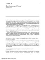
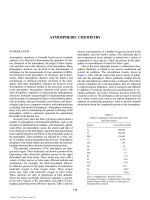
Finally, consider the robust parametric method. This starts off the
same way as the regression on order statistics method, with a
probability plot of the data after a logarithmic transformation, with a
fitted regression line (Figure 10.1). However, now instead of using the

regression line to estimate the mean and variance of the fitted
distribution, this line is extrapolated to obtain expected values for the
censored data values, as shown in Figure 10.2. For example, the
expected value for the smallest value in the sample is -5.0,
corresponding to a normal score of -2.4, the second smallest value is
-4.4, corresponding to a normal score of -2.0, and so on. The column
headed 'Fitted' in Table 10.2 gives these expected values for the order
statistics. The robust parametric method simply consists of replacing
the smallest 20 censored values for log
e
(X) with these expected
values.
Having obtained values to 'fill-in' for the censored values of log
e
(X),
these are untransformed to obtain values for X itself. The sample
mean and variance can then be calculated in the normal way. The
completed sample is shown in Table 10.3. The mean and variance
are 3.99 and 20.28, respectively, which are almost exactly the same
as the values for the real data without censoring.
© 2001 by Chapman & Hall/CRC
Figure 10.2 The regression line from Figure 10.1 extrapolated to estimate
the censored values of the logarithm of TcCB values ( denotes an
observed value of log
e
(X), and denotes an expected value from the
regression line).
Too much should not be concluded from just one example.
However, the simple substitution methods and the robust parametric
method have very definitely worked better than the alternatives here

for two reasons. First, the lognormal assumption is questionable for
the methods that require this, other than the robust method. Second,
the censored values are all very low and as long as they are replaced
by any value below the detection limit the sample mean and standard
deviation will be close to the values from the uncensored sample.
Table 10.3 The completed sample for the robust parametric method, with
the filled-in values underlined
1.33 0.04
0.09 0.28 0.08 0.11 0.07 0.47 0.14 0.12 0.07 0.04
18.40 0.02 0.02 0.01 0.01 0.03 0.05 168.6 0.11 0.25 0.25 0.06
0.48 0.26 5.56 0.05 0.29 0.31 0.33 3.29 0.33 0.34 0.37 0.25
2.59 0.39 0.40 0.28 0.43 6.61 0.48 0.10
0.49 0.51 0.51 0.38
0.92 0.60 0.61 0.43 0.75 0.82 0.85 0.13
0.94 1.05 1.10 0.54
1.53 1.19 1.22 0.62 1.39 1.39 1.52 0.33 1.73 2.35 2.46 1.10
51.97 2.61 3.06
© 2001 by Chapman & Hall/CRC
10.3 Estimation of Quantiles
It may be better to describe highly skewed distributions with quantiles
rather than using means and standard deviations. These quantiles
are a set of values that divide the distribution into ranges covering
equal percentages of the distribution. For example, the 0%, 25%,
50%, 75% and 100% quantiles are the minimum value, the value that
just equals or exceeds 25% of the distribution, the value that just
equals or exceeds 50% of the distribution (i.e., the median), the value
that just equals or exceeds 75% of the distribution, and the maximum
value, respectively.
Sample quantiles can be used to estimate distribution quantiles
that are above the detection limit, although Akritas et al. (1994) note

that simulation studies indicate that this can lead to bias when the
quantiles are close to this limit. It is therefore better to use a
parametric maximum likelihood approach when the distribution is
known. When the distribution is uncertain, the robust parametric
method can be used to 'fill-in' the censored data in the sample, before
evaluating the sample quantiles as estimates of those for the
underlying distribution of the data.
Distribution quantiles can be estimated with multiple detection
limits. See Akritas et al. (1994, Section 2.6) for more details.
10.4 Comparing the Means of Two or More Samples
The comparison of the means of two or more samples is complicated
with censored data, particularly if there is more than one detection
limit. The simplest approach involves just replacing censored data by
zero, DL, or DL/2, and then using standard methods either to test for
a significant mean difference or to produce a confidence interval for
the mean difference between the two sampled populations. In fact,
this approach seems to work quite well, and based on a simulation
study of ten alternative ways for handling censoring suggests that a
good general strategy involves substituting DL for censored values
when up to 40% of observations are censored, and substituting DL/2
when more than 40% of observations are censored (Clarke, 1994).
However, this strategy is not always the best and the United States
Environmental Protection Agency and United States Army Corps of
Engineers (1998, Table D-12) give some more complicated rules that
depend on the type of data, whether samples have equal variances,
the coefficient of variation, and the type of data distribution.
When it can be assumed that the data come from a particular
distribution, comparisons between groups can be based on the
© 2001 by Chapman & Hall/CRC
method of maximum likelihood, as described by Dixon (1998). One

of the advantages of maximum likelihood estimation is the
approximate variances and covariances of the estimators that are
available. Using these it is possible to carry out a large sample test
for whether the estimated population means are significantly different,
or to find an approximate confidence interval for this difference.
For small samples, Dixon (1998) suggests the use of bootstrap
methods for hypothesis testing and producing confidence intervals, as
discussed further in the following example. This has obvious
generalizations for use with other data distributions, and with more
than two samples. Dixon also discusses the use of non-parametric
methods for comparing samples, and the use of equivalence tests with
data containing censored values.
Example 10.2 Upstream and Downstream Samples
The data from one of the examples considered by Dixon (1998) are
shown in Table 10.4. The variable being considered is the dissolved
orthophosphate concentration (DOP, mg/l) measured for water from
the Savannah River in South Carolina, USA. One sample is of 41
observations taken upstream of a potential contamination source, and
the second sample is of 42 observations taken downstream. A higher
general level of DOP downstream is clearly an indication that
contamination has occurred. There are three DL values in this
example, <1, <5, and <10, which occurred because the DL depends
on dilution factors and other aspects of the chemical analysis that
changed during the study.
The number of censored observations is high, consisting of 26 in
each of the samples, and 63% of the values overall. Given the high
detection limit of 10 for some of the data, simple substitution methods
seem definitely questionable here, and an analysis assuming a
parametric distribution seems like the only reasonable approach.
© 2001 by Chapman & Hall/CRC

Table 10.4 Dissolved orthophosphate concentrations in samples upstream
and downstream of a possible source of contamination, with three different
detection limits
Sample 1, Upstream of Possible Contamination Source
1 2 4 3 3 <10 2 <10 <5 <10 <5 3
<5 <5 <10 <5 <10 <1 <10 7 <5 <1 <5 2
<10 5 5 <5 <10 <1 <5 <10 <5 14 5 2
<10 <10 7 <1 <10
Sample 2, Downstream of Possible Contamination Source
4 <5 <1 4 3 9 <10 4 <5 <10 <10 8
<10 3 <5 <5 <10 5 <5 <10 6 <5 1 4
<10 <5 <5 <10 5 4 2 <5 <10 <5 <10 <5
<1 <10 4 <5 20 <10
Dixon (1998) assumed that the data values X are lognormally
distributed, with log
e
(X) having the same variance upstream and
downstream of the potential source of contamination. On this basis
he obtained the following maximum likelihood estimates: mean DOP
upstream, 0.73 with standard error 0.19; mean DOP downstream,
1.02 with standard error 0.17; mean difference between downstream
and upstream, 0.24 with standard error 0.23. This clearly indicates
that the two samples could very well come from the same lognormal
distribution.
Dixon also applied parametric bootstrap methods for testing for a
significant mean difference between the upstream and downstream
samples, and for finding confidence intervals for the mean difference
between downstream and upstream. The adjective 'parametric' is
used here because samples are taken from a specific parametric
distribution (the lognormal) rather than just resampling the data with

replacement as explained in Section 4.7. These bootstrap methods
are more complicated than the usual maximum likelihood approach
but do have the advantage of being expected to have better properties
with small sample sizes.
The general approach proposed for hypothesis testing with two
samples of size n
1
and n
2
is:
(a) Estimate the overall mean and standard deviation assuming no
difference between the two samples. This is the null hypothesis
distribution.
© 2001 by Chapman & Hall/CRC
(b) Draw two random samples with sizes n
1
and n
2
from a lognormal
distribution with the estimated mean and standard deviation,
censoring these using the same detection limits as applied with the
real data.
(c) Use maximum likelihood to estimate the population means µ
1
and
µ
2
by µ
1
and µ

2
, and to approximate the standard error SE(µ
2
- µ
1
)
of the difference.
(d) Calculate the test statistic
T = (µ
2
- µ
1
)/SE(µ
2
- µ
1
),
where SE(µ
2
- µ
1
) is the estimated standard error.
(e) Repeat steps (b) to (d) many times to generate the distribution of
T when the null hypothesis is true, and declare the observed value
of T for the real data to be significantly large at the 5% level if it
exceeds 95% of the computer generated values.
Other levels of significance can be used in the obvious way. For
example, significance at the 1% level requires the value of T for the
real data to exceed 99% of the computer generated values. For a
two-sided test the test statistic T just needs to be changed to

T = |µ
2
- µ
1
|/SE(µ
2
- µ
1
),
so that large values of T occur with either large positive or large
negative differences between the sample means.
For the DOP data the observed value of T is 0.24/0.23 = 1.04. As
could have been predicted, this is not at all significantly large with the
bootstrap test, for which it was found that 95% of the computer-
generated T values were less than 1.74.
The bootstrap procedure for finding confidence intervals for the
mean difference uses a slightly different algorithm. See Dixon's
(1998) paper for more details. The 95% confidence interval for the
DOP mean difference was found to be from -0.24 to +0.71.
© 2001 by Chapman & Hall/CRC
10.5 Regression with Censored Data
There are times when it is desirable to fit a regression equation to
data with censoring. For example, in a simple case it might be
assumed that the usual simple linear regression model
Y
i
= " + $X
i
+ ,
i

holds, but either some of the Y values are censored, or both X and Y
values are censored.
There are a number of methods available for estimating the
regression parameters in this type of situation, including maximum
likelihood approaches that assume particular distributions for the error
term, and a range of non-parametric methods that avoid making such
assumptions. For more information, see the reviews by Schneider
(1986, Chapter 5) and Akritas et al. (1994).
10.6 Chapter Summary
Censored values most commonly occur in environmental data
when the level of a chemical in a sample of material is less than
what can be reliably measured by the analytical procedure.
Censored values are generally reported as being less than the
detection limit (DL).
Methods for handling censored data for the estimation of the mean
and standard deviation from a single sample include (a) the simple
substitution of zero, DL, DL/2 or a random value between zero and
DL for censored values to complete the sample; (b) maximum
likelihood methods, assuming that data follow a specified
parametric distribution; (c) regression on order statistics methods,
where the mean and standard deviation are estimated by fitting a
linear regression line to a probability plot; (d) fill-in methods, where
the mean and standard deviation are estimated from the
uncensored data and then used to predict the censored values to
complete the sample; and (e) robust parametric methods, which
are similar to the regression on order statistic methods except that
the fitted regression line is used to predict the censored values in
order to complete the sample.
© 2001 by Chapman & Hall/CRC
No method for estimating the mean and standard deviation of a

single sample is always best. However, the robust parametric
method is often best if the underlying distribution of data is
uncertain, and maximum likelihood methods (with a bias correction
for small samples) are likely to be better if the distribution is known.
An example shows good performance of the simple substitution
methods and a robust parametric method, but poor performance
of other methods when a distribution is assumed to be lognormal,
when this is apparently not true.
It may be better to describe highly skewed distributions by sample
quantiles (values that exceed defined percentages of the
distribution) rather than means and standard deviations.
Estimation of the quantiles from censored data is briefly discussed.
For comparing the means of two or more samples subject to
censoring it may be reasonable to use simple substitution to
complete samples. Alternatively, maximum likelihood can be used,
possibly assuming a lognormal distribution for data.
An example involving the comparison of two samples from
upstream and downstream of a potential source of contamination
is described. Maximum likelihood is used to estimate population
parameters of assumed lognormal distributions, with bootstrap
methods used to test for a significant mean difference, and to
produce a confidence interval for the true mean difference.
Regression analysis with censored data is briefly discussed.
© 2001 by Chapman & Hall/CRC