Statistics for Environmental Science and Management - Chapter 11 ppsx
Bạn đang xem bản rút gọn của tài liệu. Xem và tải ngay bản đầy đủ của tài liệu tại đây (141.66 KB, 8 trang )
CHAPTER 11
Monte Carlo Risk Assessment
11.1 Introduction
Monte Carlo simulation for risk assessment is a relatively new idea,
made possible by the increased computer power that has become
available to environmental scientists in recent years. The essential
idea is to take a situation where there is a risk associated with a
certain variable, such as an increased incidence of cancer when there
are high levels of a chemical in the environment. The level of the
chemical is then modelled as a function of other variables, some of
which are random variables, and the distribution of the variable of
interest is generated through a computer simulation. It is then
possible, for example, to determine the probability of the variable of
interest exceeding an unacceptable level. The description 'Monte
Carlo' comes from the analogy between a computer simulation and
repeated gambling in a casino.
The basic approach for Monte Carlo methods involves five steps:
A model is set up to describe the situation of interest.
Probability distributions are assumed for input variables, such as
chemical concentrations in the environment, ingestion rates,
exposure frequency, etc.
Output variables of interest are defined, such as the amounts of
exposure from different sources, the total exposure, etc.).
Random values from the input distributions are generated for the
input variables, and the resulting output distributions are derived.
The output distributions are summarised by statistics such as the
mean, the value exceeded 5% of the time, etc.
There are three main reasons for using Monte Carlo methods:
(1) The alternative is often to assume the worse possible case for
each of the input variables contributing to an output variable of
© 2001 by Chapman & Hall/CRC
interest. This can then lead to absurd results, such as the Record
of Decision for a US Superfund site at Oroville, California, which
specifies a clean-up goal of 5.3 x 10
-7
µg/litre for dioxin in
groundwater, which is about 100 times lower than the drinking
water standard and 20 times lower than current limits of detection
(United States Environmental Protection Agency, 1989b). Thus
there may be unreasonable estimates of risk, and unreasonable
demands for action associated with those risks, leading to the
questioning of the whole process of risk assessment.
(2) Properly conducted, a probabilistic assessment of risk gives more
information than a deterministic assessment. For example, there
may generally be quite low exposure to a toxic chemical, but
occasionally individuals may get extreme levels. It is important to
know this, and in any case the world is stochastic rather than
deterministic, so deterministic assessments are inherently
unsatisfactory.
(3) Given that a probability-based assessment is to be carried out, the
Monte Carlo approach is usually the easiest way to do this.
On the other hand, Monte Carlo methods are only really needed when
the 'worse case' deterministic scenario suggests that there may be a
problem. This is because making a scientifically defensible Monte
Carlo analysis, properly justifying assumptions, is liable to take a great
deal of time.
11.2 Principles for Monte Carlo Risk Assessment
The United States Environmental Protection Agency has put
considerable effort into the development of reasonable approaches for
using Monte Carlo simulation. Their website on this topic (United
States Environmental Protection Agency, 1999) is full of useful
information, as is their policy document (United States Environmental
Protection Agency, 1997) that can be obtained from the same source.
In the policy document the following guiding principles are stated
for Monte Carlo studies:
The purpose and scope should be clearly explained in a ‘problem
formulation’.
© 2001 by Chapman & Hall/CRC
The methods used (models, data, assumptions) should be
documented and easily located with sufficient detail for all results
to be reproduced.
Sensitivity analyses should be presented and discussed.
Correlations between input variables should be discussed and
accounted for.
Tabular and graphical representation of input and output
distributions should be provided.
The means and upper tails of output distributions should be
presented and discussed.
Deterministic and probabilistic estimates should be presented and
discussed.
The results from output distributions should be related to reference
doses, reference concentrations, etc.
It is stressed that this is a minimum set of principles that are not
intended to restrict the use of new scientifically defensible methods.
11.3 Risk Analysis Using a Spreadsheet Add-On
For many applications, the simplest way to carry out a Monte Carlo
risk analysis is using a spreadsheet add-on. Two such add-ons are
@Risk (Palisade Corporation, 2000), and Crystal Ball (Decisioneering
Inc., 2000). In both cases these products use the spreadsheet as a
basis for calculations, adding extra facilities for simulation. Typically,
what is done is to set up the spreadsheet with one or more random
input variables and one or more output variables that are functions of
the input variables. Each recalculation of the spreadsheet yields new
random values for the input variables, and consequently new random
values for the output variables. What @Risk and Crystal Ball do is to
allow the recalculation of the spreadsheet hundreds or thousands of
times, followed by the automatic generation of tables and graphs that
summarise the characteristics of the output distributions. The
following example illustrates the general procedure.
© 2001 by Chapman & Hall/CRC
Example 11.1 Contaminant Uptake Via Tapwater Ingestion
This example concerns cancer risks associated with tapwater
ingestion of Maximum Contaminant Levels (MCL) of
tetrachloroethylene in high risk living areas. It is a simplified version
of a case study considered by Finley et al. (1993).
A crucial equation gives the dose of tetrachloroethylene received
by an individual (mg/kg-day) as a function of other variables. This
equation is
Dose = (C x IR x EF x ED)/(BW x AT) (11.1)
where C is the chemical concentration in the tapwater (mg/litre), IR is
the ingestion rate of water (litres/day), EF is the exposure frequency
(days/year), ED is the exposure duration (years), BW is the body
weight (kg), and AT is the averaging time (days). The numerator is
the total dose received in EF x ED exposure days, while the
denominator is the total number of days in the period considered.
Dose is therefore the average daily dose of tetrachloroethylene per
kilogram of body weight. The aim in this example is to determine the
distribution of this variable over the population of adults living in a high
risk area.
The variables on the right-hand side of equation (11.1) are the
input variables for the study. These are assumed to have the
following characteristics:
C, the chemical concentration, is assumed to be constant at the
MCL for the chemical of 5 µg/litre;
IR, the ingestion rate of tapwater, is assumed to have a mean of
1.1 and a range of 0.5-5.5 litres per day, based on survey data;
EF, the exposure frequency, is set at the United States
Environmental Protection Agency upper point estimate of 350
days per year;
ED, the exposure duration, is set at 12.9 years based on the
average residency tenure in a household in the United States;
BW, the body weight is assumed to have a uniform distribution
between 46.8 (5th percentile female in the United States) and
101.7 kg (95th percentile male in the United States); and
AT, the averaging time, is set at 25,550 days (70 years).
© 2001 by Chapman & Hall/CRC
Thus C, EF, ED and AT are taken to be constants, while IR and
BW are random variables. It is, of course, always possible to argue
with the assumptions made with a model like this. Here it suffices to
say that the constants appear to be reasonable values, while the
distributions for the random variables were based on survey results.
For IR the empirical distribution shown in Table 11.1 is used because
this gives the correct mean and range.
Table 11.1 Distribution used for the ingestion rate of
tapwater for the individuals living in high risk areas
Ingestion rate (l/day) Probability
0.50 0.2857
0.75 0.2571
1.00 0.2286
1.50 0.0857
2.00 0.0571
2.50 0.0286
3.00 0.0143
3.50 0.0143
4.00 0.0114
4.50 0.0086
5.00 0.0057
5.50 0.0029
Total 1.0000
There are two output variables:
Dose, the dose received (mg/kg-day) as defined before; and
ICR, the increased cancer risk (the increase in the probability of
a person getting cancer) which is set at Dose x CPF(oral),
where CPF(oral) is the cancer potency factor for the
chemical taken orally.
For the purpose of the example CPF(oral) was set at the United
States Environmental Protection Agency's upper limit of 0.051.
A spreadsheet was set up containing dose and ICR as functions of
the other variables, with the @Risk add-on activated. Each
recalculation of the spreadsheet then produced new random values
for IR and BW, and consequently for dose and ICR, to simulate the
situation for a random individual from the population at risk. The
number of simulated sets of data was set at 10,000. Table 11.2
© 2001 by Chapman & Hall/CRC
shows some of the summary output obtained (minimums, maximums,
means, etc.), while Figure 11.1 shows the distribution obtained for the
ICR. (The dose distribution is the same but with the horizontal axis
divided by 0.051.)
The 50th and 95th percentiles for the ICR distribution are 0.05x10
-5
and 0.20 x 10
-5
, respectively. Finlay et al. (1993) note that the 'worse
case' scenario gives an ICR of 0.53 x 10
-5
, but a value this high was
never seen with the 10,000 simulated random individuals from the
population at risk. Hence the 'worse case' scenario actually
represents an extremely unlikely event. At least, this is the case
based on the assumed model.
Figure 11.1 Simulated distribution for the increased cancer risk as obtained
from the output of @RISK.
© 2001 by Chapman & Hall/CRC
Table 11.2 Summary of output from @Risk
based on simulating 10,000 random individuals
from the population living in a high
contamination area
Name Dose*10
-5
ICR*10
-5
Description Output Output
Cell A35 C35
Minimum = 0.4344 0.0222
Maximum = 10.2119 0.5208
Mean = 1.3778 0.0703
Std Deviation = 1.1539 0.0588
Variance = 1.3314 0.0035
Skewness = 2.7076 2.7076
Kurtosis = 11.9364 11.9364
Errors Calculated = 0 0
Mode = 1.1234 0.0573
5% Perc = 0.4795 0.0245
10% Perc = 0.5348 0.0273
15% Perc = 0.6042 0.0308
20% Perc = 0.6671 0.0340
25% Perc = 0.7069 0.0361
30% Perc = 0.7560 0.0386
35% Perc = 0.8141 0.0415
40% Perc = 0.8748 0.0446
45% Perc = 0.9161 0.0467
50% Perc = 0.9746 0.0497
55% Perc = 1.0509 0.0536
60% Perc = 1.1452 0.0584
65% Perc = 1.2516 0.0638
70% Perc = 1.3708 0.0699
75% Perc = 1.5357 0.0783
80% Perc = 1.7690 0.0902
85% Perc = 2.1374 0.1090
90% Perc = 2.6868 0.1370
95% Perc = 3.8249 0.1951
11.4 Further Information
A good starting point for more information is the Risk Assessment
Forum home page (United States Environmental Protection Agency,
2000). For examples of a range of applications of Monte Carlo
methods, a special 400 page issue of the journal Human and
Ecological Risk Assessment will be useful (Association for the
Environmental Health of Soils, 2000). For more information about
@Risk, see the book by Winston (1996).
© 2001 by Chapman & Hall/CRC
11.5 Chapter Summary
The Monte Carlo method uses a model to generate distributions for
output variables from assumed distributions for input variables.
These methods are useful because 'worse case' deterministic
scenarios may have a very low probability of ever occurring,
stochastic models are usually more realistic, and Monte Carlo is
the easiest way to use stochastic models.
The guiding principles of the United States Environmental
Protection Agency for Monte Carlo analysis are summarised.
An example is provided to show how Monte Carlo simulation can
be done with the @RISK add-on for spreadsheets.
Sources of further information are noted.
© 2001 by Chapman & Hall/CRC