WETLAND PLANTS: BIOLOGY AND ECOLOGY - CHAPTER 6 doc

Part III
Wetland Plant Communities:
Function, Dynamics, Disturbance
L1372 - Chapter 6 04/25/2001 9:39 AM Page 189
© 2001 by CRC Press LLC
6:
The Primary Productivity of Wetland Plants
I. Introduction
The primary productivity of many wetlands is quite high especially when compared to
other natural communities or even to highly managed agricultural croplands (Table 6.1).
A high value for the aboveground primary productivity of swamps and marshes in tem-
perate zones is about 3500 grams dry weight per square meter per year (g m
-2
yr
-1
). In cold
wetlands and peat bogs an upper limit of about 1000 g m
-2
yr
-1
is typical (Bradbury and
Grace 1993). Wetlands with emergent herbaceous vegetation are often more productive
than other wetland types, although high values are found in some mangrove swamps as
well (Table 6.2). Wetland primary productivity depends upon the type of wetland and the
vegetation found there as well as on hydrology, climate, and environmental variables such
as soil type and nutrient availability. Wetlands that receive nutrient subsidies either natu-
rally from flooding or from farm runoff tend to be more productive than those that receive
nutrients only from rainwater, such as scrub cypress swamps or ombrotrophic bogs
(Brown 1981). In a highly productive freshwater marsh in Wisconsin (from 2800 to 3800 g
m
-2

yr
-1
), the soil nutrients were found in higher concentrations than in upland soils and
in excess of what is needed for agricultural crops (Klopatek and Stearns 1978).
Still water wetlands such as bogs or scrub cypress swamps have low primary produc-
tivity (100 to 300 g m
-2
yr
-1
), but they may perform essential ecological functions by sup-
porting wildlife or rare plant species or they may be sites of important storages of water or
peat (Brown 1981). The salt marshes of the arctic and subarctic are among the least pro-
ductive of coastal wetlands. Nonetheless, they are valuable as vital staging areas for large
populations of migrating waterfowl (Roberts and Robertson 1986).
A. Definition of Terms
The terms used to report primary productivity results for wetland habitats are sometimes
used interchangeably, making it difficult to directly compare the results from different
studies. Some researchers have argued for the adoption of standard terms and methods;
most studies use the terms as defined here (Wetzel 1964, 1966, 1983a; Wetzel and Hough
1973; Westlake 1975, 1982; Aloi 1990).
1. Standing Crop
Standing crop (synonymous with standing stock) is the dry weight of a plant population
on any given date. The term maximum standing crop denotes the maximum dry weight of
L1372 - Chapter 6 04/25/2001 9:39 AM Page 191
© 2001 by CRC Press LLC
plants during the season. Strictly speaking, standing crop applies to only aboveground
plant parts, so the term should not be used when the belowground portions of the plants
are also sampled (Wetzel 1966; Wetzel 1983a).
2. Biomass
The term biomass is in wider use for ecological studies than standing crop. The biomass of

a plant is its dry weight in grams. The biomass of a tree, for example, includes the weight
of flowers + fruits + leaves + current twigs + branches + stems + roots (Brinson et al. 1981).
If only the aboveground portions of the plant are measured, then this should be specified
and called aboveground biomass. The biomass of a community is usually reported as grams
of dry weight in an area (g m
-2
). Dry weight is determined by drying plant matter in a dry-
ing oven usually for 24 to 72 h at temperatures from 60 to 105˚C.
Sometimes biomass is reported as ash-free dry weight (AFDW; synonymous with organic
dry weight). Ash-free dry weight is determined by combusting dried plant matter in a
TABLE 6.1
The Annual Aboveground Primary Productivity of Different
Ecosystem Types (units are g dry weight m
-2
yr
-1
)
Mean Net
Primary
Ecosystem Type Productivity
Swamp and marsh 2500
Tropical rain forest 2000
Tropical seasonal forest 1500
Temperate evergreen forest 1300
Temperate deciduous forest 1200
Boreal forest 800
Savanna 700
Agricultural land 644
Woodland and shrubland 600
Temperate grassland 500

Lake and stream 500
Tundra and alpine 144
Desert scrub 71
Rock, ice, and sand 3
Weighted average land NPP 720
Algal bed and reef 2000
Estuaries 1800
Upwelling zones 500
Continental shelf 360
Open ocean 127
Weighted average ocean NPP 153
Average for biosphere 320
Data from Colinvaux 1993.
L1372 - Chapter 6 04/25/2001 9:39 AM Page 192
© 2001 by CRC Press LLC
combustion oven at 550˚C for 15 min. The organic carbon present in the plant tissues is
released as a gas. The difference between the original dry weight of the material and its weight
after combustion is roughly the weight of the organic matter, or the ash-free dry weight.
3. Peak Biomass
Peak biomass occurs when vegetation is at its highest biomass. After peak biomass, growth
declines and the vegetation dies. Production studies often report peak biomass as the pro-
duction for the growing season, even though much of the plants’ production is unrecorded
with this method (Wiegert and Evans 1964).
4. Primary Production
Primary production is the conversion of solar energy into chemical energy. The process of
energy transformation, or photosynthesis, is a complex set of biochemical reactions that
can be expressed in simple terms as a chemical equation:
light energy
6CO
2

+ 12H
2
O > C
6
H
12
O
6
+ 6O
2
+ 6H
2
O (6.1)
chlorophyll
Carbon dioxide and water are the raw materials necessary for the production of a simple
carbohydrate (glucose), with the evolution of oxygen and the release of water as by-
products.
In ecological studies, primary production is measured and reported as (Colinvaux
1993):
• Biomass, reported as the weight in grams of the dry matter produced by plants
• Mass of an element, such as the amount of oxygen evolved or the amount of
TABLE 6.2
A Range of Net Aboveground Primary Productivity Values for Different
Wetland Types
Net Primary
Productivity
Wetland Type (g dry wt m
-2
yr
-1

)
Salt marsh 130–3700
Tidal freshwater marsh 780–2300
Freshwater marsh
a
900–5500
Mangrove 1270–5400
Southeastern bottomland hardwood 830–1610
Cypress swamp 200–1540
Forested northern peatland
a
260–2000
Non-forested northern peatland
a
100–2000
a
Above- and belowground production.
Note: Most of the data are from North American wetlands (data from Mitsch and
Gosselink 2000; some values were converted from g C to g dry weight assuming
carbon is 45% of dry weight).
L1372 - Chapter 6 04/25/2001 9:39 AM Page 193
© 2001 by CRC Press LLC
carbon fixed during photosynthesis, expressed in grams of oxygen or carbon or
in terms of moles of the element
• Energy (calories produced or joules consumed in production)
In most wetland studies, primary production results are reported as amounts of bio-
mass produced. Plant biomass reflects net primary production and does not include losses
to respiration, excretion, secretion, injury, death, or herbivory.
To determine net primary production from biomass, it is necessary to measure plant
biomass more than once. The change in biomass between two measurements is equal to

the net production for that time period. Net production is calculated from biomass as fol-
lows (Newbould 1970):
B
1
Biomass of a plant community at a certain time t
1
B
2
Biomass of the same community at t
2
∆B = B
2
– B
1
Biomass change during the period t
1
– t
2
L Plant losses by death and shedding during t
1
– t
2
G Plant losses to consumer organisms such as
herbivorous animals, parasitic plants, etc. during t
1
– t
2
P
n
Net production by the community during t

1
– t
2
If the amounts, DB, L, and G, are successfully estimated, we can calculate P
n
as the sum
P
n
= ∆B + L + G (6.2)
5. Respiration
Respiration is the process by which a plant cell oxidizes stored chemical energy in the form
of sugars, lipids, and proteins and converts the energy released into a chemical form
directly usable by cells (e.g., ATP). The equation for the respiration of glucose is essentially
the reverse of Equation 6.1. During respiration the plant requires oxygen and releases car-
bon dioxide. Unlike photosynthesis, respiration takes place in both the light and the dark.
In most ecological studies, respiration is measured in the dark as the evolution of carbon
dioxide by the plant (usually enclosed in a gas chamber) or by the decrease in oxygen con-
centration surrounding the plant (Grace and Wetzel 1978). Respiration is usually
expressed as an hourly rate and then multiplied by 24 for a daily rate under the assump-
tion that daytime and nighttime respiration rates are equal. This assumption is probably
false, since the daytime work of photosynthesis probably brings about a higher rate of res-
piration. Nonetheless, this assumption is often used in primary production studies and the
underestimate of respiration that it represents is considered to be minimal.
Respiration can represent a high proportion of the gross productivity of a plant.
Brinson and others (1981) reported the average respiration rate measured in nonforested
wetlands to be 72% of gross primary productivity. Respiration rates change over time and
are influenced by climatic variables. In a Florida riverine marsh, respiration was higher
during the rainy season (77% of gross primary productivity) than during the cooler dry
season (50% of gross primary productivity; Brinson et al. 1981). Respiration increases with
higher temperatures or increasing rates of primary productivity, probably because of the

increased availability of labile photosynthetic products.
L1372 - Chapter 6 04/25/2001 9:39 AM Page 194
© 2001 by CRC Press LLC
6. Primary Productivity
Primary productivity is primary production over time, or the rate of primary production. If
gaseous exchange methods are used to measure primary productivity, the time period is a
day or an hour and the units are grams of oxygen evolved or carbon assimilated. In wet-
land macrophyte studies, results are usually given in units of dry plant matter production
per unit area per year (g dry weight m
-2
yr
-1
). In the temperate zone, growth per year is
actually growth during the growing season. It is important to specify the length of the
growing season since it can be quite long in low latitudes and short in high latitudes.
a. Gross Primary Productivity
Gross primary productivity (GPP) is the measured change in plant biomass plus all of the
predatory and nonpredatory losses (respiration) from the plant divided by the time inter-
val. It includes all of the new organic matter produced by a plant plus all that is used or
lost during the same time interval (Wetzel 1983a). It can be defined as the sum of daytime
photosynthesis and day- and nighttime respiration (Brinson et al. 1981).
b. Net Primary Productivity
Net primary productivity (NPP) is the observed changes in plant organic matter over a time
period. NPP is GPP minus all losses (such as respiration and herbivory). It is the value
most often reported in wetland macrophyte production studies. Other terms and abbrevi-
ations for NPP are used in the literature that may be more precise because they include
modifying terms such as annual (thereby giving the term a rate component), aboveground,
aerial, or shoot (which indicate which portion of the biomass was measured). Some of
these terms are:
• NAPP: net aerial primary production. Although rate is not implied in this term,

reports are generally for 1 year of growth (Linthurst and Reimold 1978a, b;
Groenendijk 1984; Cahoon and Stevenson 1986; Hik and Jefferies 1990; Dai and
Wiegert 1996)
• ANPP: aboveground annual net primary production (Kistritz et al. 1983)
• NAAP: net annual aboveground production (Dickerman et al. 1986; Wetzel and
Pickard 1996)
• ANPPs: annual net primary shoot production (Jackson et al. 1986)
7. Turnover
Turnover is the amount of biomass lost during the growing season (to leaf loss, herbivory, or
other causes). The turnover rate is turnover (g m
-2
yr
-1
), divided by peak biomass (g m
-2
). It
is expressed in units of year
-1
, which reflects the calculation involved (g m
-2
yr
-1
divided by
g m
-2
). Peak biomass (an underestimate of net primary productivity) can be corrected for
leaf loss by multiplying by the turnover rate.
Leaf turnover is sometimes estimated for emergent plants so that peak biomass can be
corrected for the weight of leaves that have been lost, dropped, or consumed, or that have
died on the plant. Leaf turnover is determined by dividing the total number of leaves pro-

duced per shoot per year by the modal number of leaves per shoot per year (the mode is the
value that occurs most frequently in a series of observations). Dickerman and others (1986)
calculated leaf turnover in a Michigan Typha latifolia stand to be 1.38 leaves leaf
-1
yr
-1
.
Morris and Haskin (1990) showed that by adding leaf turnover to peak biomass of Spartina
alterniflora, the result for NPP was 20 to 38% greater than peak biomass alone.
L1372 - Chapter 6 04/25/2001 9:39 AM Page 195
© 2001 by CRC Press LLC
8. P/B Ratio
The P/B ratio is a measure of the amount of energy flow relative to biomass (Wetzel 1983a).
The P/B ratio is unitless and it is estimated as the ratio of net primary productivity (P) to
peak biomass (B). The P/B ratio is usually assumed to be equivalent to the turnover rate.
In theory, however, the P/B ratio is greater than the turnover rate since the value for P
includes turnover as well as the net production that occurs after peak biomass (Grace and
Wetzel 1978). Typical values for P/B ratios in submerged plants are 1.0 to 2.0 (Kiorboe
1980; Wetzel 1983a). For emergents P/B ratios range from 0.3 to 7.0, with most values less
than 1.0 (calculated from data in Wetzel 1983a). For large trees, P/B ratios are low (<0.5)
since productivity of the wood and leaves in a single year is less than the total biomass of
the tree (Brinson et al. 1981). If a P/B ratio for a species has been well established in other
studies, researchers sometimes measure peak biomass and multiply it by the P/B ratio to
estimate NPP (Kiorboe 1980).
B. Reasons for Measuring Wetland Primary Productivity
1. To Quantify an Ecosystem Function
An understanding of primary production is essential to the understanding of ecosystem
functions (Reader and Stewart 1971; Gholz 1982; Kemp et al. 1986; Dame and Kenny 1986;
Meyer and Edwards 1990). All of the heterotrophic organisms in a community depend on
the energy supplied by plants. Primary productivity data are often the basis for quantita-

tive studies of other ecosystem processes. Knowledge of oxygen and carbon fluxes can
provide insight into the cycling and retention of other elements as well as the redox con-
ditions in wetland water and soil. For example, primary producers retain nutrients during
the growing season, and release them as they senesce. The mass of nutrients taken up by
plants can be estimated from measurements of primary productivity and a knowledge of
nutrient concentrations in plant tissue. Other pathways of nutrient removal (i.e., sedimen-
tation or denitrification) can be estimated by the difference in plant uptake and the mass
of the nutrients that remains. Information about productivity and nutrient fluxes is vital to
ecosystem modelers who wish to describe an ecosystem’s functions and make predictions
about its future (Mitsch and Reeder 1991).
The primary productivity of wetlands is of particular interest because it provides a link
between terrestrial communities and downstream aquatic ecosystems. Wetland plants use
nutrients that flow into their habitat from upstream areas. The detritus generated by wet-
land plants may be carried out of the wetland into downstream waters where it is broken
down and consumed. The plant matter produced in wetlands is vital both within the wet-
land and downstream. With wetland primary productivity measurements and informa-
tion on hydrology, researchers are able to quantify the wetland’s contribution to down-
stream ecosystems (Cahoon and Stevenson 1986).
2. To Make Comparisons within a Wetland
Results from primary productivity studies within a single wetland can reveal temporal
and spatial patterns of growth and changes from year to year. If primary productivity
studies are undertaken in wetlands that are subject to disturbance, such as water resource
projects (Johnson and Bell 1976), fire (Ewel and Mitsch 1978), added nutrients (Mitsch and
Ewel 1979; Brown 1981), impoundment (Conner et al. 1981; Conner and Day 1992), silvi-
cultural activities (Gholz 1982), acid deposition (Rochefort et al. 1990), or the installation
of roads or structures (Visser and Sasser 1995), the results can reveal the environmental
L1372 - Chapter 6 04/25/2001 9:39 AM Page 196
© 2001 by CRC Press LLC
impact of the disturbance. Such studies can also help managers and planners prepare for
changes due to future disturbances (Bartsch and Moore 1985).

Primary productivity studies have been used to monitor the development of plant
communities in constructed wetlands (Fennessy et al. 1994a; Cronk and Mitsch 1994a,
1994b; Niswander and Mitsch 1995). In the case of disturbed or constructed wetlands, pri-
mary productivity measurements can answer questions regarding the status of the ecosys-
tem (i.e., whether the wetland is recovering from disturbance, responding to new inputs,
or developing as a new wetland).
3.To Make Comparisons among Wetlands
Comparisons among wetlands allow us to generalize about primary productivity within
categories of wetlands. For example, we usually expect the productivity of freshwater
marshes in warm climates to exceed that of ombrotrophic bogs. When similar wetlands
have different primary productivity results, the researcher is prompted to seek explana-
tions for the differences.
The primary productivity of a restored or constructed wetland can be compared to that
of nearby natural wetlands of the same type. The researcher can then begin to determine
whether the new wetland is functioning like a natural one (Confer and Niering 1992; see
Case Study 6.A, Salt Marsh Productivity: The Effect of Hydrological Alterations in Three
Sites in San Diego County, California).
4.To Determine Forcing Functions and Limiting Factors of Primary Productivity
Variations in light, hydrology, nutrients, salinity, or substrate act to promote or limit plant
growth in a particular site or type of wetland. Comparisons of the wetland type in different
locations help distinguish the environmental and climatic variables that influence produc-
tivity. One reason that primary productivity is high in many wetlands is simply that the envi-
ronment is favorable for growth. The plants are not under water stress, there are sufficient
nutrients, and the wetland is located in an area with a suitable climate for plant growth.
Many wetland primary productivity studies and reviews have established that hydrol-
ogy is a major forcing function in wetlands (Mitsch and Ewel 1979; Zedler et al. 1980;
Brinson et al. 1981; Brown 1981; Grigal et al. 1985; Lugo et al. 1988; Brown 1990; Cronk and
Mitsch 1994a). The source and amount of incoming water determine the structure and
function of wetlands. Water can be nutrient-rich or nutrient-poor; it can arrive in the wet-
land as a gentle rain or a tidal surge. In general, the primary productivity of nontidal wet-

lands is higher with greater water throughflow (Brinson et al. 1981). For tidal wetlands,
productivity is influenced by both tidal flushing and freshwater inputs from upland, with
greater productivity in sites that receive substantial freshwater runoff (Lugo et al. 1988; see
Chapter 3, Section II.B.1, Hydrology and Primary Productivity).
II. Methods for the Measurement of Primary Productivity in Wetlands
Many quantitative methods are available for wetland primary productivity studies, in part
because wetlands encompass a variety of habitats. Methods have been adapted from both
aquatic and terrestrial ecology. A combination of methods is sometimes used within a single
study because several plant forms (e.g., algae, submerged, emergent, and floating-leaved
plants) coexist within the wetland. Gas exchange techniques are usually used for the algal
component of the community, harvest and biomass methods are used for macrophytes, and
forestry techniques are used to determine the primary productivity of wetland trees.
L1372 - Chapter 6 04/25/2001 9:39 AM Page 197
© 2001 by CRC Press LLC
Conclusions about a wetland’s status or about its response to human-induced impacts
are sometimes based on productivity studies, so it is critical to understand the methods
used and to identify sources of error (Bradbury and Hofstra 1976). Difficulties in inter-
preting primary productivity measurements stem from the variety of methods used both
within a single wetland for the different plant forms as well as among different studies
(Talling 1975). It is difficult to compare primary productivity results generated with very
different methods, sampling intervals, plot sizes, and conversion factors. The choice of
methods depends on the type of plant community to be measured, as well as on the time,
resources, and labor available. In wetland macrophyte primary productivity studies, most
of the published results are from the harvest of vegetation that has an annual growth cycle.
Sometimes plants are harvested once, at the end of a growth cycle. The growth cycle is usu-
ally based on the dominant species in the wetland. Alternatively, plants are measured sev-
eral times throughout the growing season and their productivity is calculated from the
findings at each sampling date. Some of the errors associated with these procedures
include (Brinson et al. 1981; Dickerman et al. 1986; Bradbury and Grace 1993):
• Statistical error based on the number of samples. Statistically valid measurements of

vegetation often require large sample sizes in many plots. Insufficient sample
size can result in large statistical error.
• Errors based on the frequency of sampling. Estimates of production rates depend on
the frequency of sampling throughout the growing season. More frequent sam-
pling often results in higher estimates because less plant production is missed
due to death, herbivory, and decay.
• Errors due to plant mortality. Some methods miss a large proportion of production
because they fail to include biomass that dies between sampling periods or
before peak biomass has occurred.
• Errors due to seasonality of measurements. Productivity is assumed to be zero
between the end of one growing season and the beginning of the next. However,
this assumption may not be valid, because growth continues throughout the year
in the warmest areas of the temperate zone and in the subtropics and tropics
(Hopkinson et al. 1978; Dai and Wiegert 1996).
• Errors due to the omission (or unstated inclusion) of more than one of the plant com-
ponents of the wetland. Primary productivity estimates often reflect only the pro-
ductivity of the dominant plant form in a community, such as the most common
macrophytes or trees. If the productivity of other members of the plant commu-
nity have been measured, such as phytoplankton, periphyton, epiphytes, vines,
or the understory of forests, sometimes it is not clear whether these have been
included in figures for total productivity. These values should be subtracted from
total productivity when comparing to studies in which these measurements were
not made.
• The omission of belowground biomass. Researchers frequently measure only
aboveground biomass. Many wetland plants are long-lived perennials, with con-
siderable belowground biomass, and failing to measure it can result in large
underestimates of wetland productivity. Not all studies warrant this extra effort,
especially if the goal is to determine effects of an aboveground phenomenon
such as grazing or to compare to other studies of only aboveground results.
In this section we briefly describe several, although not all, of the primary productiv-

ity methods commonly used in wetland studies. The plant components of wetlands that
L1372 - Chapter 6 04/25/2001 9:39 AM Page 198
© 2001 by CRC Press LLC
we discuss are phytoplankton (floating algae), periphyton (attached algae), submerged
plants, emergent plants, floating and floating-leaved plants, trees, shrubs, and moss.
Although phytoplankton, periphyton, and moss are not the primary focus of our book, we
include them here because of their importance in the primary productivity of the entire
wetland plant community.
A. Phytoplankton
At any given time, algal standing stock is generally much smaller than that of macro-
phytes. Nonetheless, algae can constitute a high proportion of the annual primary pro-
ductivity of an aquatic community. Algae have a high P/B ratio (>100; Wetzel 1983a) and
can quickly take advantage of nutrient inputs. In addition, when higher plants are dor-
mant during the winter, algal productivity may continue, thus increasing the relative con-
tribution of algae to the total productivity of the system (Pomeroy and Wiegert 1981).
Fontaine and Ewel (1981) showed that the plankton community of a shallow Florida lake
contributed 44% of the total primary production for the system. Mitsch and Reeder (1991)
found phytoplankton activity represented over 80% of primary production in a fresh-
water estuarine marsh adjacent to Lake Erie in Ohio. In four constructed emergent
marshes in Illinois, phytoplankton contributed from 17 to 67% of the primary production
of the wetlands (Cronk and Mitsch 1994a).
Several methods have been developed to measure phytoplankton primary productiv-
ity. We briefly describe two of them here. The first is the measurement of dissolved oxygen
released during photosynthesis. The second is the measurement of carbon uptake during
photosynthesis.
1. Dissolved Oxygen Concentration
The amount of dissolved oxygen present in water results from photosynthetic and respi-
ratory activities of aquatic biota and from diffusion at the air–water interface (Odum 1956;
Copeland and Duffer 1964; Lind 1985). Since dissolved oxygen concentrations fluctuate on
a daily and seasonal basis, several measurements over time are necessary for an estimate

of the system’s productivity (Odum 1956; Penfound 1956; Jervis 1969). The method is
based on the fact that oxygen is released into the water as a result of photosynthetic pri-
mary production during the day, and it is taken up throughout both the night and the day
by autotrophic and heterotrophic organisms and by chemical oxidation.
a. Diurnal Dissolved Oxygen Method
Starting at dawn, oxygen production begins in response to daylight. On sunny days, oxy-
gen production increases throughout the morning and early afternoon and then decreases
before or at sunset. In this method, data are collected every 2 to 3 h during a 24-h period
(from dawn on day 1 to dawn on day 2). Water samples are taken at pre-determined depths
and poured into glass bottles designed for the measurement of biochemical oxygen demand
(BOD; Figure 6.1). The dissolved oxygen concentration is determined with a dissolved oxy-
gen meter, or with a chemical reaction known as the Winkler method (A.P.H.A. 1995).
Alternatively, fully submersible dissolved oxygen meters with data loggers are left in place
at the study site, and readings are taken as frequently as the researcher desires (although
these data include oxygen production of submerged macrophytes and periphyton).
A plot of the results vs. time reveals the peak of oxygen production during the day as
well as the nightly shutdown of oxygen production. The area under the curve represents
the NPP of the phytoplankton sampled. The hourly rate of respiration (determined from
L1372 - Chapter 6 04/25/2001 9:39 AM Page 199
© 2001 by CRC Press LLC
the oxygen decrease during the night) is multiplied by 24 h and added to NPP for an esti-
mate of GPP. Nighttime respiration is assumed to be equal to daytime respiration,
although this may be a source of error since daytime respiration may exceed respiration in
the dark by an unknown amount. Another source of error in the estimate for respiration
comes from the inclusion of heterotrophs in the water sample. Their respiratory con-
sumption is included in the measurement. The results of the diurnal method are expressed
as mg O
2
l
-1

d
-1
. Results are multiplied by 1000 to convert to g O
2
m
-3
d
-1
and then multi-
plied by the depth at the sampling station for an areal result in g O
2
m
-2
d
-1
.
The diurnal method has been applied to many wetland and shallow aquatic systems,
such as Narragansett Bay in Rhode Island (Nixon and Oviatt 1973), the Chesapeake Bay in
Maryland (Kemp and Boynton 1980), the Illinois Fox Chain of Lakes (Mitsch and
Kaltenborn 1980), a Florida lake (Fontaine and Ewel 1981), a Lake Erie coastal wetland in
Ohio (Mitsch and Reeder 1991), a Georgia river (Meyer and Edwards 1990), and fresh-
water constructed wetlands in Illinois (Cronk and Mitsch 1994a).
b. Light Bottle/Dark Bottle Dissolved Oxygen Method
The light bottle/dark bottle technique provides estimates of GPP, NPP, and respiration
based on incubated samples (Wetzel 1983a; Wetzel and Likens 1990). In this method, at
least four water samples are taken at each depth under study. Two samples are kept in clear
glass BOD bottles, and one in a BOD bottle darkened with aluminum foil or other opaque
material. The fourth sample from each depth is analyzed for dissolved oxygen content
immediately. This is the initial concentration (IB). The remaining light and dark samples
are suspended in the water column at the depths from which they were taken, or they are

kept in the laboratory under similar light and temperature conditions. The time of incuba-
tion must be sufficient for a change to occur (usually from 1 to 4 h). In highly productive
waters typical of many wetlands, the incubation period can be shorter than in oligotrophic
waters (more typical of deep lakes). During incubation, the dissolved oxygen in the light
bottles should increase due to photosynthetic production of oxygen. The dissolved oxygen
in the dark bottles should decrease from respiratory consumption of oxygen.
After incubation, the dissolved oxygen concentration within the bottles is determined.
The average concentration of the two light bottles (LB) is greater than the original concen-
tration (IB) and the difference is equal to the amount of oxygen produced:
(LB – IB) = NPP (6.3)
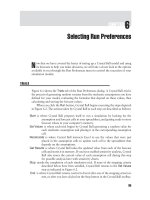
FIGURE 6.1
Biochemical oxygen demand bottles used for the
measurement of oxygen production and consumption to
estimate the primary productivity of phytoplankton.
Shown are one ‘light’ bottle and one bottle darkened
with aluminum foil and tape. (Photo by H. Crowell.)
L1372 - Chapter 6 04/25/2001 9:39 AM Page 200
© 2001 by CRC Press LLC
The concentration of the dark bottle (DB) is subtracted from the original concentration (IB),
to yield a rate of respiration:
(IB – DB) = respiration (6.4)
The sum of the differences is the GPP:
(LB – IB) + (IB – DB) = GPP (6.5)
To express the results as a daily rate of productivity (mg O
2
l
-1
d
-1
), samples are incu-

bated for several 1- to 4-h periods from dawn to dusk. The results are plotted on a graph
of time vs. productivity. The area under the curve for the day’s measurements is divided
by the area under the curve for a 1- to 4-h incubation period. This ratio provides a factor
by which the shorter incubation time is expanded to a daily value (Wetzel and Likens
1990).
In the light bottle/dark bottle method, it is assumed that respiration is the same in the
light and dark bottles. As for the diurnal oxygen method above, it is impossible to take a
sample containing only phytoplankton, so the respiration rate includes that of bacteria and
zooplankton. Isolating the samples in bottles also creates problems with “container
effects” in which the environment is altered by excluding grazers, nutrients, and atmos-
pheric exchange processes. The results from incubated samples may therefore be an under-
estimate of production (Hall and Moll 1975; Schindler and Fee 1975).
2. Carbon Assimilation: The
14
C Method
During photosynthesis, plants assimilate inorganic carbon and transform it into organic
carbon compounds. In the
14
C method, the amount of inorganic carbon taken up by plants
is measured and the results are expressed as a mass of carbon per unit volume per time
interval (mg C m
-3
time
-1
).
Samples are taken at various depths or locations within the water column of the wet-
land. At the beginning of the sampling period, a portion of a sample is analyzed for alka-
linity and pH (see A.P.H.A. 1995). The rest of the sample is poured into one dark and two
light BOD bottles and a small amount of
14

C in the form of radioactive bicarbonate
(NaH
14
CO
3
) is added to each using a syringe. The bottles are incubated for 3 to 4 h during
the middle of the day at the depth from which they were taken. The dark bottle inhibits
photosynthesis and the rate of carbon uptake should be close to zero. At the end of the
incubation period, the amount of labeled carbon (
14
C) that has been taken up in the phy-
toplankton is measured. The total amount of carbon assimilated is proportional to the
amount of
14
C taken up. The average result for the light bottles minus the result for the
dark bottle reflects the photosynthetic incorporation of carbon during the incubation
period (C m
-3
h
-1
; Lind 1985; Wetzel and Likens 1990).
The result can be converted to daily rates by incubating samples for several 4-h periods
throughout the day. As in the light bottle/dark bottle method, the ratio of the productiv-
ity for the day to the productivity for the shorter incubation period provides a factor by
which to correct the hourly rate and estimate a daily rate (Wetzel and Likens 1990).
The
14
C method is more sensitive than the method of measuring oxygen change (Wetzel
1983a; Lind 1985). The smallest amount of photosynthesis that can be detected with dis-
solved oxygen readings is about 20 mg C m

-3
h
-1
, while the
14
C method is sensitive to changes
as small as 0.1 to 1 mg C m
-3
h
-1
(Wetzel 1983a). In wetlands, this level of sensitivity may not
be necessary since the water column is often highly productive. Instruments and supplies for
the
14
C method are expensive, more training is necessary than for the oxygen method,
L1372 - Chapter 6 04/25/2001 9:39 AM Page 201
© 2001 by CRC Press LLC
analysis is not completed in the field, and some researchers have warned that results may
underestimate GPP (Lind 1985; Stevenson 1988; Aloi 1990; Colinvaux 1993).
B. Periphyton
Periphyton are attached algae that may be found on nearly any submerged surface. More
specific terms for periphyton are based on whether they are attached to inorganic or
organic substrates (Aloi 1990):
• Epilithon: periphyton on rock substrates
• Epipelon: periphyton on mud or silt substrates
• Episammon: on sand substrates
• Epiphyton: on the submerged portions of aquatic macrophytes
In oceans, deep lakes, and downstream areas of rivers, phytoplankton dominates produc-
tivity, but when the ratio of sediment area to water volume increases, as is the case in wet-
lands, the macrophytes and periphyton become more significant contributors to the sys-

tem’s productivity (Sand-Jensen and Borum 1991). Periphyton are known to be significant
producers in salt marshes, with productivity estimates ranging from 10 to 25% of macro-
phyte productivity in east coast U.S. salt marshes (Pomeroy 1959; Gallagher and Daiber
1974; Van Raalte et al. 1976; Pomeroy and Wiegert 1981) and 80 to 140% of macrophyte
productivity in southern California salt marshes (Zedler, 1980). The higher ratios recorded
in California are due to both higher algal production and lower macrophyte production.
Twilley (1988) found that epiphytic algae took up as much as 16% of the total carbon fixed
in mangrove wetlands of Florida and Puerto Rico. In four constructed freshwater marshes,
from 1 to 37% of the primary productivity was attributed to periphyton, with the highest
levels in wetlands with higher hydrologic throughflow (Cronk and Mitsch 1994b).
The literature concerning periphyton primary productivity is replete with variations in
methodology (Wetzel 1983b; Robinson 1983; Aloi 1990). Periphyton primary productivity
can be measured much like that of phytoplankton, i.e., as the evolution of oxygen or the
uptake of carbon. Changes in periphyton biomass over time can also give an estimate of
periphyton NPP. Biomass changes may be assessed using either natural or artificial sub-
strates.
Natural substrates include rocks, macrophytes, and other underwater surfaces. To
measure epilithon biomass in wetlands, rocks are collected and the attached algal growth
is scraped off of the surface and then dried and weighed. To remove epiphyton from
macrophytes, the macrophyte is placed in a jar with water and shaken. After shaking, the
plants are gently scraped (Aloi 1990).
Artificial substrates are often used in periphyton studies to provide a uniform area and
a means with which to control environmental variables. Artificial substrates provide a stan-
dard means of comparison between two sites with the benefit of decreased cost of sampling,
decreased disruption of habitat, and decreased time required to obtain a quantitative sam-
ple (Aloi 1990). Suitable artificial substrates are uniform in size, shape, and material.
Materials are chosen in part for their resistance to the effects of prolonged submersion.
Many investigators have introduced artificial substrates such as microscope slides made of
glass (many studies starting in 1916 as cited by Aloi 1990) or plastic (Figure 6.2; Cronk and
Mitsch 1994b; Wu and Mitsch 1998), clay tiles (Barko et al. 1977), nutrient diffusing sand

agar surfaces (Pringle 1987, 1990), or cylindrical rods of different textures (Goldsborough
and Hickman 1991; Hann 1991). Substrates that can be suspended vertically are often
L1372 - Chapter 6 04/25/2001 9:39 AM Page 202
© 2001 by CRC Press LLC
preferable in order to minimize the accumulation of inorganic solids (Aloi 1990). Artificial
substrates are useful in studies of colonization, community development, herbivory, or in
the comparison of the effects of an environmental variable or different habitats. They are
less useful in primary productivity studies because they do not imitate naturally occurring
growth and the algal species that grow on artificial substrates are not necessarily the same
as those on natural substrates (Wetzel 1964, 1966, 1983a; Wetzel and Hough 1973).
Periphyton are harvested from a portion of the substrates at regular time intervals (for
example, every 2 weeks) in order to detect initial colonization, as well as a peak and
decline in growth (Carrick and Lowe 1988; APHA 1995). Colonization of introduced sub-
strates generally occurs at an exponential rate for the first 2 weeks of exposure and then
slows (Kevern et al. 1966; Lamberti and Resh 1985; Paul and Duthie 1988). Biomass
measurements of periphyton are made by drying and weighing samples. Another com-
mon measure of periphyton biomass is ash-free dry weight because periphyton samples
often include inorganic matter that could skew dry weight results upward. Biomass mea-
surements provide an underestimate of NPP because they do not account for losses due to
herbivory, sloughing, or dislodgement (Aloi 1990).
Periphyton NPP may be more accurately estimated by measuring gas exchange tech-
niques. Rocks or other periphyton substrates are incubated in bottles and either the oxy-
gen or
14
C method is used (as described for phytoplankton). Disturbing the community
may skew productivity findings due to changes in flow regime and nutrient supply, so
some researchers measure productivity in situ by enclosing the substrate in clear plastic
chambers pushed into the substrate or in domes sealed to large rock surfaces. The cham-
ber is left to incubate for a certain length of time and then changes in oxygen or carbon are
measured. Measuring epiphytic productivity is more complicated because enclosing the

substrate means that the productivity of the macrophyte substrate as well as the
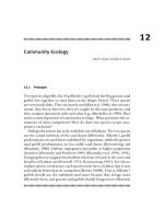
FIGURE 6.2
Periphyton sampler made of PVC pipe and plastic microscope slides from
which slides were removed every 2 weeks during the growing season in order
to assess the colonization rate, biomass accumulation, and community struc-
ture at four constructed wetlands near the Des Plaines River, Illinois. (From
Cronk, J.K. and Mitsch, W.J. 1994b. Aquatic Botany 48: 325–342. Reprinted with
permission.)
L1372 - Chapter 6 04/25/2001 9:39 AM Page 203
© 2001 by CRC Press LLC
periphyton will be measured. Often, epiphytes are scraped or shaken from the plant and
placed in bottles for incubation; however, the effects of this disturbance on productivity are
not known (Twilley et al. 1985; Aloi 1990).
C. Submerged Macrophytes
The biomass of submerged macrophytes is measured by direct harvest or by incubating
the plants and measuring oxygen production or carbon fixation.
1. Biomass
The biomass of submerged macrophytes is measured by harvesting and drying plants.
Because they are underwater, the method is somewhat more involved than for emergent
macrophytes. Plots of known area are placed randomly within an aquatic plant bed.
Harvesting is usually carried out at the estimated peak biomass. If the depth of the site
warrants, sampling is done by SCUBA divers. The plants are sorted, cleaned of sediments
and periphyton, and dried in a drying oven at 70˚ to 105˚C to a constant weight.
Belowground biomass is estimated by collecting sediment cores, weighing the sorted,
washed, and dried roots, and then extrapolating for the rest of the community.
Peak biomass is sometimes used as the estimate for that year’s net production, or sam-
ples are taken through the growing season and net production is calculated as the sum of
the positive biomass increments until peak biomass. Alternatively, peak biomass is
measured and then multiplied by published values for P/B ratios. Examples of P/B ratios
are 1.2 for Potamogeton pectinatus, 2.0 for Ruppia cirrhosa and R. maritima, 2.0 for

Myriophyllum spicatum, and 1.16 for Ranunculus baudauti (from various sources cited by
Kiorboe 1980). Peak biomass values may be difficult to determine for submerged species.
For example, M. spicatum peaks earlier in shallow water than in deep water. Therefore,
peak biomass for M. spicatum should be determined at different times depending upon
water depth (Grace and Wetzel 1978).
2. Oxygen Production
To measure oxygen production by submerged plants, samples are harvested and cleaned
of epiphytes and sediment. They are placed in light and dark BOD bottles and filled with
water taken from the same site that has been filtered to remove algae. They are incubated
at the approximate depth from which the sample was pulled and periodically shaken to
reduce boundary-layer effects (an intact boundary layer can result in a decrease of nutri-
ents near the plant surface). The incubation period is from 1 to 4 h. The dissolved oxygen
in the bottles is measured using the same methods described for phytoplankton.
Productivity is calculated as for the light bottle/dark bottle method for phytoplankton.
The disturbances inherent in this method can produce considerable error in the results.
Plants are severed from their roots, which is the source of most of their nutrients. They are
brought to the surface, exposed to intense surface light, and then returned to their original
depth, thus imposing abnormal light and flow conditions (Wetzel 1964). NPP results are
higher if only apical portions of the plant are used rather than lower parts of the plant. NPP
may be underestimated because oxygen produced photosynthetically fills the plant’s lacu-
nae first, before it is released to the water (Wetzel 1966; Sondergaard 1979). For Potamogeton
perfoliatus the lag time between initial light and the initial evolution of oxygen to the water
has been measured at 5 to 25 min (Kemp et al. 1986). If oxygen is measured after the plant
has been exposed to light for at least a few minutes, the error introduced into production
L1372 - Chapter 6 04/25/2001 9:39 AM Page 204
© 2001 by CRC Press LLC
estimates by lag time is reduced. Respiration in the light and dark bottles is usually
assumed to be equal (Kemp et al. 1986).
3. Carbon Assimilation
Samples are collected in the same manner as for dissolved oxygen measurements.

Radioactive bicarbonate is added to the bottles and the analysis and calculation of produc-
tivity are the same as described in the
14
C method for phytoplankton. Results are expressed
as the weight of carbon fixed per dry biomass weight per unit time (g C g
-1
h
-1
) and incu-
bation is generally 4 to 5 h (Wetzel 1966).
D. Emergent Macrophytes
The bulk of wetland primary productivity studies have been done in emergent marshes,
so more methods exist for emergents than for other types of wetland plants. The primary
productivity of emergent plants can be measured using gas exchange methods by enclos-
ing the plants in clear chambers in which the changes in gas concentrations are monitored
(Mathews and Westlake 1969; Blum et al. 1978; Pomeroy and Wiegert 1981; Brinson et al.
1981; Jones 1987; Bradbury and Grace 1993). However, most researchers use biomass meth-
ods and we describe several of these methods below.
1. Aboveground Biomass of Emergent Plants
Many researchers have compared aboveground emergent production methods in salt
marshes (Kirby and Gosselink 1976; Turner 1976; Linthurst and Reimold 1978b; Gallagher
et al. 1980; Hardisky 1980; Hopkinson et al. 1980; Shew et al. 1981; Groenendijk 1984;
Houghton 1985; Dickerman et al. 1986; Jackson et al. 1986; Cranford et al. 1989; Kaswadji
et al. 1990; Morris and Haskin 1990; Dai and Wiegert 1996) and freshwater marshes
(Dickerman et al. 1986; Wetzel and Pickard 1996; Daoust and Childers 1998), yet a defini-
tive method does not exist (Table 6.3). The comparison studies show that NPP results
depend on the method chosen and they can vary up to sixfold (Table 6.4; Linthurst and
Reimold 1978b). With such wide variation in the results, the choice of method can have
important consequences.
The methods described here are based on measurements of plant biomass. The data are

collected by harvesting, drying, and weighing plants. Alternatively, plant growth in study
plots is monitored and biomass is estimated using regressions of height (or other parame-
ters) to weight based on plants harvested outside of the plots. Production is expressed in
grams dry weight per square meter and productivity is usually reported as a yearly rate
(g dry weight m
-2
yr
-1
). Losses to respiration are not included so the results are a measure
of NPP. The variation in the methods we describe arises from the inclusion of different
components of the plant community (live, dead, decomposed matter) and from various
ways of calculating NPP. The choice of method depends upon the plant community and
on environmental and time constraints. We describe eight commonly used methods, but
others are available. We use the names for these methods that are the most frequently used
in the literature. Some have descriptive names while others use the originators’ names:
Peak biomass Milner and Hughes (1968)
Valiela et al. (1975) Smalley (1959)
Wiegert and Evans (1964) Lomnicki et al. (1968)
Allen curve method (1951) Summed shoot maximum
L1372 - Chapter 6 04/25/2001 9:39 AM Page 205
© 2001 by CRC Press LLC
TABLE 6.3
Some Methods for the Measurement of Net Aboveground Primary Productivity of Emergent Herbaceous Wetland Plants and Evaluations
of the Methods Made in Comparisons or Reviews
Method Calculation of Net Primary Productivity Evaluation Evaluated by
Peak biomass Maximum biomass Underestimate Numerous studies; see text
Milner and Hughes (1968) Sum of positive changes in live biomass Underestimate Linthurst and Reimold 1978b
Shew et al. 1981
Dickerman et al. 1986
Morris and Haskin 1990

Best estimate using Dai and Wiegert 1996
tagged plants
Invalid method Daoust and Childers 1998
Valiela et al. (1975) Sum of changes in dead biomass plus an Underestimate Valiela et al. 1975
estimate for biomass decayed during sampling Linthurst and Reimold 1978b
interval Dickerman et al. 1986
Dai and Wiegert 1996
Smalley (1959) Sum of changes in live and dead biomass Underestimate Linthurst and Reimold 1978b
or, if sum is negative, equal to zero Shew et al. 1981
Dickerman et al. 1986
Cranford et al. 1989
Daoust and Childers 1998
Wiegert and Evans (1964) Sum of changes in live and dead biomass plus an Best estimate Kirby and Gosselink 1976
estimate for biomass decayed during sampling Groenendijk 1984
interval Over- or underestimate Linthurst and Reimold 1978b
Overestimate Hopkinson et al. 1980
Shew et al. 1981
Dickerman et al. 1986
Dai and Wiegert 1996
Daoust and Childers 1998
L1372 - Chapter 6 04/25/2001 9:39 AM Page 206
© 2001 by CRC Press LLC
© 2001 by CRC Press LLC
Lomnicki et al. (1968) Sum of changes in live biomass plus the dead biomass Overestimate, but slight Shew et al. 1981
measured at the end of each sampling interval modification was best
estimate (see text)
Allen curve method (1951) Area beneath curve of shoot density vs. average Slight underestimate, Dickerman et al. 1986
shoot biomass for estimates of plants growing as not appropriate to all
cohorts; requires new curve for each new cohort plant types
Good estimate Cranford et al. 1989

Overestimate; for use Bradbury and Grace 1993
with plants that develop
in recognizable cohorts
Underestimate if plants Wetzel and Pickard 1996
have continuously
emerging new shoots
Summed shoot maximum Sum of the maximum biomass for each shoot in Best estimate Dickerman et al. 1986
study plot
L1372 - Chapter 6 04/25/2001 9:39 AM Page 207
© 2001 by CRC Press LLC
© 2001 by CRC Press LLC
TABLE 6.4
Studies That Compared Results for the Estimation of Net Aboveground Primary Productivity of Wetland Emergents Using Various Measurement
and Calculation Methods (units are g dry weight m
-2
yr
-1
)
Productivity Plant Species Location Peak Milner and Valiela Smalley Wiegert and Lomnicki Allen Summed
Study Biomass Hughes et al. Evans et al. Curve Shoot
Maximum
Kirby and Gosselink Spartina alterniflora Louisiana 788 748 1006 1323
1976 (short)
S. alterniflora (tall) 1018 874 1410 2645
Linthurst and S. patens Maine 912 912 2523 3523 5833
Reimold 1978b
a
S. patens Delaware 807 522 1241 980 2753
S. patens Georgia 946 705 1028 1674 3925
Gallagher et al. Juncus roemerianus Georgia 2500 2800

1980 S. alterniflora (short) 700 1500
S. alterniflora (tall) 2300 3000
Hardisky 1980 S. alterniflora N. Carolina 931
Hopkinson et al. Distichlis spicata Louisiana 900 900 750 2800
1980 J. roemerianus 1200 1800 1250 3200
Sagittaria falcata 550 1000 600 1300
S. alterniflora 700 1500 1000 2200
S. cynosuroides 750 300 1100 1600
S. patens 1200 2500 2000 5800
Shew et al. 1981 S. alterniflora N. Carolina 242 214 225 1029 1028
Groenendijk 1984
b
Elytrigia pungens Netherlands 474–878 1416–1787
Spartina anglica 1162–1649 2139–2659
Houghton 1985
c
S. alterniflora (short) New York 780 770 750 825
S. alterniflora (tall) 1220 1310 1460 1400
Jackson et al. 1986
d
S. anglica England 160–180 590–760
Dickerman et al. Typha latifolia Michigan 768 –836 764–834 1557–1346 1604–1284 2762–2266
1986
e
(harvested plots)
T. latifolia 833–1318 833–1317 834–1301 927–1358 1005–1507
(study plots)
L1372 - Chapter 6 04/25/2001 9:39 AM Page 208
© 2001 by CRC Press LLC
© 2001 by CRC Press LLC

Cranford et al. 1989
f
S. alterniflora Nova Scotia 398 434 507
Kaswadji et al. 1990 S. alterniflora 831 831 1231 1873 1437
Morris and Haskin S. alterniflora S. Carolina 209–694 295–820 402–1042
1990
g
(short)
Dai and Wiegert S. alterniflora Georgia 1105 993 1118
1996
h
(short)
S. alterniflora (tall) 1520 1315 1557
Wetzel and Pickard T. latifolia Lab 120–267 214–232 345–696
1996
i
Daoust and Childers Cladium jamaicense Florida 944 2315 3593
1998
j
Wet prairie: 165 319 531
8 dominant emergents
Average ratio of method’s results to peak biomass (±1 S.D.) 1.0 ± 0.2 2.0 ± 0.6 1.6 ± 1.0 3.3 ± 1.2 3.0 ± 1.8 1.2 ± 0.4 1.9 ± 0.7
Note: Methods are discussed in the text.
a
Linthurst and Reimold 1978b: measured the NPP of other species, but only one is shown here to illustrate the different results among the methods.
b
Groenendijk 1984: range is for different calculations used for each method.
c
Houghton 1985: measured for 2 years, just 1 year’s results are reported here.
d

Jackson et al. 1986: range is for 2 years of data.
e
Dickerman et al. 1986: data from the most frequent time interval used in their calculations; range is for 2 years; the first year’s data are both > and < the second year’s data,
depending on the method.
f
Cranford et al. 1989: modified the Smalley and Allen curve methods slightly.
g
Morris and Haskin 1990: range is for 5 years of data.
h
Dai and Wiegert 1996: used Milner and Hughes and Valiela et al. calculation methods with tagged plants in permanent quadrats rather than harvested plants.
i
Wetzel and Pickard 1996: also used other methods not described here; range is for five different experimental treatments.
j
Daoust and Childers 1998: used these computational methods in combination with phenometric techniques specific to the species in their study.
L1372 - Chapter 6 04/25/2001 9:39 AM Page 209
© 2001 by CRC Press LLC
© 2001 by CRC Press LLC
A general trend within the productivity literature has been to include more components of
the plant or plant community in the measurements. The later methods tend to be more
complex or more time-consuming as a result of these trends. The changes are an effort to
more accurately estimate NPP. Most of the methods have been applied to stands of
Spartina alterniflora (cordgrass) and Typha latifolia (broad-leaved cattail), so the methods
here are probably most appropriate for monospecific stands of monocots. Areas with more
diversity and those containing eudicots present problems to which researchers must adapt
these methods.
a. The Peak Biomass Method
The primary productivity of emergent plants can be estimated by harvesting and weigh-
ing the aboveground portion of plants when they are at peak biomass. Peak biomass usu-
ally occurs in mid- to late summer in temperate areas. In subtropical and tropical zones, it
can be difficult to detect peak biomass because growth continues throughout the year.

In this method, samples are selected either randomly, along transects within commu-
nities, within a specific moisture gradient, or according to other physical features of inter-
est. At peak biomass, plant shoots within a plot, or quadrat (usually from 0.1 to 1 m
2
) are
clipped at the sediment surface. The plant matter is dried and weighed and results are
expressed as g dry weight m
-2
. NPP is usually expressed as yearly growth or growth per
number of days of the growing season. In some studies, plants are harvested or monitored
several times throughout the growing season and the greatest value is taken as the peak
biomass. Frequent sampling enables the investigator to detect the time of peak biomass
more accurately than with a single measurement (Boyd 1971; Boyd and Vickers 1971). The
peak biomass method is simple to apply, requires minimal field and laboratory time, and
the results are comparable from season to season within the same site.
The disadvantage of this method is that it does not provide a good estimate of NPP. The
fact that peak biomass is almost always an underestimate of NPP, sometimes by several-
fold, has been confirmed in many studies (Wiegert and Evans 1964; Wetzel 1966; Valiela et
al. 1975; Bradbury and Hofstra 1976; Kirby and Gosselink 1976; Linthurst and Reimold
1978b; Whigham et al. 1978; Shew et al. 1981; Westlake 1982; Houghton 1985; Dickerman
et al. 1986; Jackson et al. 1986; Dai and Wiegert 1996; Wetzel and Pickard 1996). This
method does not include corrections for plant mortality before peak biomass, nor does it
include any production that occurs after peak biomass. It also does not take into account
any differences in the time at which different species attain peak biomass (Wiegert and
Evans 1964). In most temperate wetlands, plants die during the winter and each year’s
plant growth is distinguishable from the previous year’s crop (Nixon and Oviatt 1973).
However, in warm areas, plant growth may occur throughout the year. The peak biomass
method does not subtract carry-over live plant material that was present before the begin-
ning of the current growing season (Linthurst and Reimold 1978b).
This method is not used as frequently now as it was in earlier ecological studies due to

these problems. When it is used, the results should be clearly designated as peak biomass
or maximum standing crop. Despite the method’s drawbacks, use of the peak biomass
method can be justified under some circumstances:
• Cost: It may be the only method that researchers can afford since it requires less
effort than other methods.
L1372 - Chapter 6 04/25/2001 9:39 AM Page 210
© 2001 by CRC Press LLC
• Comparison among multiple sites: When many sites are to be compared, it may be
the only feasible method. For example, van der Valk and Bliss (1971) measured
the peak biomass of emergent plants in 15 oxbow wetlands in Alberta, Canada.
They sampled three times so as to detect peak biomass. Their goal was to com-
pare the same parameter (peak biomass) among many wetlands rather than to
report the primary productivity.
• Difficult access to sites: If the study site is difficult to access, sampling more than
once during the growing season may be impractical. For example, Glooschenko
(1978) studied a remote subarctic salt marsh in northern Ontario and reported
results as aboveground biomass rather than productivity.
• Subarctic sites: The use of the peak biomass method in the preceding example
(Glooschenko 1978) was also appropriate because peak biomass more accurately
reflects true primary production in cold climates than it does in temperate zones
(Hopkinson et al. 1980). During the short subarctic growing season, less turnover
of plant tissues occurs, so there are fewer unaccounted losses. Thus, the accuracy
of peak biomass measurements increases with increasing latitude.
• Long-term study within a single marsh or area: In a Netherlands salt marsh, the use
of the peak biomass method by De Leeuw and others (1990) was justified because
their goal was to compare results within the same marsh over a long time period.
They measured peak biomass annually for 13 years. They acknowledged that
their results are an underestimate of NPP, and they did not attempt to compare
their results to those of other salt marshes.
b. The Milner and Hughes Method

In the Milner and Hughes (1968) method, NPP is calculated as the sum of the increases in
live biomass between successive sampling dates. Dead biomass is not included in the sum.
The results are for the growing season and expressed as g dry weight m
-2
yr
-1
. Usually
plants are harvested each month during the growing season, and so this method is some-
times called “summation of the new monthly growth” (Morris and Haskin 1990; Dai and
Wiegert 1996). The Milner and Hughes method yields results that are very similar to peak
biomass results, particularly if all shoots die in the fall (Table 6.4; Dickerman et al. 1986).
Results are less than peak biomass if plants continue to grow throughout the winter
because live biomass remaining from the preceding growing season is subtracted from the
sum for the current season (Kirby and Gosselink 1976; Linthurst and Reimold 1978b).
This method has been evaluated as an underestimate of NPP by several researchers
(Table 6.3; Linthurst and Reimold 1978b; Shew et al. 1981; Dickerman et al. 1986; Morris
and Haskin 1990). Daoust and Childers (1998) determined that the Milner and Hughes
method was invalid for their study because their results with this method differed signif-
icantly from results obtained using other calculation methods. The results from the Milner
and Hughes method are not corrected for mortality or loss of plant parts that occurs dur-
ing the growing season (Dickerman et al. 1986). In monotypic communities, the method
misses the peak of younger cohorts that may occur after the first peak in biomass. In
diverse plant communities, the method misses the maximum growth of species that start
and peak at different times, compared to the dominant species.
The Milner and Hughes method has been used in a number of studies (Smith et al. 1979;
Cargill and Jefferies 1984; Dai and Wiegert 1996), particularly in salt marshes, where
monotypic stands of Spartina alterniflora resemble the grasslands for which this method
was designed. Results from a subarctic salt marsh probably come close to actual NPP, since
the rates of leaf turnover and decomposition are low in cold climates with short growing
L1372 - Chapter 6 04/25/2001 9:39 AM Page 211

© 2001 by CRC Press LLC
seasons (Cargill and Jefferies 1984). Dai and Wiegert (1996) used a modified version of this
method in which tagged plants of a single species were monitored closely throughout the
growing season. They concluded that the results of this method were their best estimate
for primary production because the method closely tracked actual growth.
c. The Valiela et al. Method
In the Valiela et al. (1975) method, NPP is calculated as the total of dead material measured
over a growing season. This method was devised to measure the NPP of a Spartina alterni-
flora salt marsh in Massachusetts. Since standing crops varied little from year to year at
their site, the researchers assumed that the dead matter that accumulated over a growing
season was equal to net annual aboveground production. At each sampling period, they
harvested and separated live and dead material. They also calculated losses that may have
occurred due to decomposition during the sampling interval. The decomposed biomass
was calculated as follows:
• If there is less dead material at the end of the sampling interval than at the begin-
ning, then the change in dead material is a negative value. The absolute value of
the loss in dead material is the amount of decomposed biomass. In the form of
an equation, the decomposed biomass (e) is calculated as follows:
e = –∆ d, if ∆ l ≥ 0 and ∆ d < 0 (6.6)
where ∆ l is the change in live standing crop between any two sampling dates,
and ∆ d is the change in standing dead matter for the same interval.
• If living plant material decreases during the sampling period, then the absolute
value of the sum of the change in living material and the change in dead mater-
ial is equal to the decomposed biomass (e):
e = – (∆ l + ∆ d), if ∆ l < 0 (6.7)
Net primary production for each sampling interval is calculated as the sum of dead mate-
rial plus the amount calculated for the decomposed biomass (e). NPP for the growing sea-
son is the sum of the values for each sampling interval.
Results from this method are usually considered an underestimate of NPP because
when there is an increase in live material, concomitant mortality, and no apparent change

in the standing dead material, then growth is unassessed for that period. In addition, if
dead material is washed away by tides, it is not counted in the method (Valiela et al. 1975).
The Valiela et al. method is appropriate where the litter component is negligible and
where the wetland is in a steady state with the rate of production balanced by the rate of
decomposition (Dickerman et al. 1986). Dai and Wiegert (1996) modified the Valiela et al.
method by summing the monthly dead biomass and correcting it for the net change of aer-
ial living biomass between the beginning and the end of the growing season (their site was
in Georgia, where growth continued during the winter). They monitored the same plants
throughout the growing season. The height of the plants was measured, and biomass was
determined from a regression of plant height on plant weight. The height of standing dead
plants was used to estimate biomass. However, the height of the dead plants was less than
that of their maximum live height, so biomass was underestimated.
L1372 - Chapter 6 04/25/2001 9:39 AM Page 212
© 2001 by CRC Press LLC
d. The Smalley Method
To measure the NPP of Spartina alterniflora in a Georgia salt marsh, Smalley (1959) devised
a method in which the biomass of both the live and dead material within quadrats is mea-
sured several times throughout the growing season. The changes in both live and dead bio-
mass from one sampling period to the next determine how net production for that sam-
pling interval is to be determined. The conditions for calculating net production are:
• If the change in living material is positive and the change in standing dead is pos-
itive, then net production is their sum.
• If both are negative, then net production is zero.
• If the change in living material is positive and the change in standing dead is neg-
ative, then net production is equal to the change in living material.
• If the change in standing dead is positive and the change in living material is neg-
ative, the two values are added for net production, but if the sum is negative,
then net production is zero.
NPP for this method is the sum of net production results for each sampling period
expressed per unit time (g m

-2
yr
-1
).
The Smalley method has been used in emergent wetland studies (Zedler et al. 1980;
Kistritz et al. 1983) and tested against other methods by many researchers (Table 6.4; Kirby
and Gosselink 1976; Turner 1976; Linthurst and Reimold 1978b; Gallagher et al. 1980;
Hardisky 1980; Hopkinson et al. 1980; Shew et al. 1981; Groenendijk 1984; Houghton 1985;
Jackson et al. 1986; Dickerman et al. 1986; Cranford et al. 1989; Kaswadji et al. 1990; Daoust
and Childers 1998). The general conclusion from these studies is that the results are an
underestimate of NPP (Table 6.3). Several reasons are given:
• The Smalley procedure does not correct for the instantaneous loss of plant litter
(i.e., the plant material that is lost to decomposition during the sampling inter-
val; Dickerman et al. 1986).
• Since negative values are reported as zero, the magnitude of change from one
sampling period to the next is unknown. Negative net production is considered
a contradiction in terms. Even though it is measured, it is disregarded for that
sampling period. However, the errors in the estimate of the actual amounts of
live and dead material present are carried forward and are not corrected (Turner
1976).
• In tidal marshes there is often export of dead leaf material, which is not measured
in this method. The amount may be large (up to 35% of production) or small
(where plants have a low rate of leaf loss; Kistritz et al. 1983).
• Tides can also import dead material into a study plot, but this added material
does not represent growth within the plot (Linthurst and Reimold 1978b).
e. The Wiegert and Evans Method
The Wiegert and Evans method (1964) originally was devised for grassland studies. The
method corrects for one of the sources of error in the Smalley method (namely, the instan-
taneous loss of litter). The Wiegert and Evans method sums the live and dead material pro-
duced during each sampling interval and it adds an estimate for the decomposed plant

material. The decomposed biomass is estimated as a proportion of the dead biomass for
L1372 - Chapter 6 04/25/2001 9:39 AM Page 213
© 2001 by CRC Press LLC
each sampling period. Samples are usually taken once per month for a year or a growing
season. NPP is the sum of the monthly values.
The changes in standing live vegetation and the changes in mortality are measured from
one sampling period to the next. Mortality is the change in dead material plus the material
that has decomposed. To determine NPP for any given time interval using this method, the
following six parameters are needed (standing crop data are expressed in g m
-2
; instanta-
neous rates in mg g
-1
d
-1
):
Let t
i
= a time interval (in days)
a
i – 1
= standing crop dead material at start
a
i
= standing crop dead material at end
b
i – 1
= standing crop live material at start
b
i

= standing crop live material at end
r
i
= instantaneous daily rate of disappearance of dead material during interval
These parameters are used to calculate the amount of dead material that disappears dur-
ing an interval (x
i
):
x
i
= (a
i
+ a
i - 1
) / 2 × r
i
t
i
(6.8)
The change in standing crop of live material is
∆ b
i
= b
i
– b
i - 1
(6.9)
The change in standing crop of dead material is
∆ a
i

= a
i
– a
i - 1
(6.10)
Since ∆ a
i
is the change in dead standing crop during the interval, then (x
i
+ ∆ a
i
) is the
amount of material added to the dead standing crop during the interval, i.e., the mortality
of live material, symbolized here by d
i
:
d
i
= x
i
+ ∆ a
i
(6.11)
The last equation must be ≥ 0; negative values indicate an error in one or more of the
measured parameters.
The growth during a given time interval (t
i
) is then given by:
y
i

= ∆ b
i
+ d
i
(6.12)
where y
i
is expressed in grams per unit area.
These equations are used to calculate the mortality and growth of the vegetation for
each sampling period. The amounts for each period are summed and expressed per unit
time for NPP.
The estimate of the instantaneous loss of litter (r) needed for the Wiegert and Evans
method is obtained using one of two procedures. The first is the paired-plot method in
which each study plot is paired with a second plot that is identical in size and as similar to
the first in vegetation size and type as possible. The dead material is removed from the first
plot and weighed (W
i - 1
) at the initial sampling time (t
i - 1
). At the same time, the live mate-
rial is removed from the second plot, leaving only dead material. At the second sampling
time (t
1
), the dead material from the second plot is removed and weighed (W
1
). The instan-
taneous rate of disappearance of dead material from these plots is estimated as:
L1372 - Chapter 6 04/25/2001 9:39 AM Page 214
© 2001 by CRC Press LLC