LANDSCAPE ECOLOGY A Top-Down Approach - Chapter 11 pdf
Bạn đang xem bản rút gọn của tài liệu. Xem và tải ngay bản đầy đủ của tài liệu tại đây (709.96 KB, 16 trang )
© 2000 by CRC Press LLC
11
A Land Transformation Model for the Saginaw
Bay Watershed
Bryan C. Pijanowski, Stuart H. Gage, David T. Long,
and William E. Cooper
CONTENTS
Introduction
Project Objectives
Conceptual Elements
Spatial Framework
Spatial Class Hierarchies
Spatial Interactions
Resolution
Spatial Scaling
State Transitions
Landscape Features
Number of Subdrivers
GIS Framework
GIS Integration Schematic
Model Interface
Model Application
Site Description
Pilot LTM Driving Variables
Results and Discussion
Acknowledgments
© 2000 by CRC Press LLC
Introduction
A suite of complex factors, including policy, population change, culture, eco-
nomics, and environmental characteristics, drive land use change. Land use
change is one of the most critical dynamic elements of ecosystems (e.g., Baker
1989; Richards 1992; Riebsame et al. 1994; Bockstael et al. 1995). Human-
induced changes to the land often result in changes to patterns and processes
in ecosystems such as alterations to the hydrogeochemistry (Flintrop et al.
1996), vegetation cover (e.g., Ojima et al. 1994), species diversity (Costanza et
al. 1993), and changes to the economies of a community. It is for these reasons
that issues surrounding land use are central to the concerns of local and
regional resource managers and community land use planners.
Information about current land use patterns, the causes of land use change,
and the subsequent effects of these changes can be effectively communicated
to resource managers, community planners, and policy analysts using geo-
graphic information systems, predictive models, and decision support sys-
tems (Cheng et al. 1996; Doe et al. 1996). The advancements in many
geographic information system applications such as ARC/INFO (Environ-
mental Systems Research Institute 1996) and the increased accessibility of
spatial databases makes developing simulation models within geographic
information systems more feasible than even a few years ago.
This paper presents an overview of the modeling framework, systems
approach, and spatial class hierarchies of our pilot, GIS-based Land Transfor-
mation Model (LTM). Our LTM has been developed to integrate a variety of
land use change driving variables, such as population growth, agricultural
sustainability, transportation, and farmland preservation policies for the Sag-
inaw Bay Watershed (SBW) in Michigan. The pilot LTM utilizes a set of spa-
tial interaction rules, which are organized into an object class hierarchy. The
model is entirely coded within a geographic information system with graph-
ical user interfaces that allow users to change model parameters. Output of
the LTM includes a time series of projected land uses in the watershed at
user-specified timesteps.
Project Objectives
The objectives of the Land Transformation Project are to: develop a spa-
tial–temporal model that characterizes land use change in large regions; cre-
ate a model that is transferable in scope to other regions undergoing land
transformation; incorporate policy, socioeconomics, and environmental fac-
tors driving land use change; develop a pilot LTM that demonstrates proof of
© 2000 by CRC Press LLC
concept and that can be used to generate spatial and temporal aspects that
can be generalized for the development of new model components; apply a
systems approach to model development; and use the model to test “what-
if” policy scenarios.
Conceptual Elements
The LTM (Pijanowski et al. 1995, 1996, in review) describes the influence of
land use change on ecosystem integrity and economic sustainability of large
regions. Conceptually, the LTM contains six interacting modules (Figure
11.1): (1) Policy Framework; (2) Driving Variables; (3) Land Transformation;
(4) Intensity of Use; (5) Processes and Distributions; and (6) Assessment End-
points. All modules and submodules within the conceptual diagram are rec-
ognized not to be mutually exclusive; we use this diagram to illustrate main
points and provide a foundation for the description of more detailed model
components. The pilot LTM that is described below contains two of the six
LTM modules, driving variables and land transformation. The spatial extent
of the LTM can be any definable region; however, because future model
developments will be focused on coupling land use change and hydrogeo-
logic and geochemical processes, we give precedence to watersheds as the
spatial extent in LTM applications.
The Policy Framework module of the LTM organizes the goals for the
stakeholders of the watershed who include resource managers, private and
corporate landowners, and local land use planners. Stakeholder goals may
include: control of pollutant inputs, ecological restoration, habitat preserva-
tion, improving biodiversity and biological integrity, and facilitating eco-
nomic growth. Within this framework, many stakeholder goals are under
certain types of constraints (e.g., economic, environmental), are made with
certain expectations of outcomes, and with specific spatial and temporal
scales in mind. For example, a township land use planner is likely to be mak-
ing decisions within his/her own township. Likewise, a state or federal gov-
ernment resource manager might be concerned about areas that encompass
several counties.
The LTM contains three general categories (Figure 11.1) of Driving Vari-
ables: Management Authority, Socioeconomics, and Environmental. Man-
agement Authority includes the institutional components and policies of
land use. Land ownership is an important component in this module of the
model since state and federally owned lands (e.g., state and federal forests,
parks, and preserves) need to be excluded from development. Socioeconomic
driving variables include population change, economics, of land ownership,
transportation, agricultural economics, and locations of employment. Envi-
ronmental driving variables of land transformation are (1) abiotic, such as the
distribution of soil types and elevation, and (2) biotic, such as the locations of
endangered and threatened species, or the attractiveness of certain types of
vegetation patterns in the landscape for development. Driving variables may
© 2000 by CRC Press LLC
contain intercorrelated subcomponents; hence the model can be hierarchical.
For example, the farming socioeconomic system in the SBW application of
the pilot model is composed of farm-size dependent economics, farmer
demographics, and environmental influences on farm productivity.
Land Transformation is characterized by change in land use and land
cover. Land use describes the anthropogenic uses of land as it affects ecolog-
ical processes and land value (Veldkamp and Fresco 1996). Land uses that we
consider at the most general level are urban, agriculture/pasture, forest, wet-
lands, open water, barren, and nonforested vegetation. Land cover character-
izes the plant cover of associated land use and is thus not mutually exclusive
of land use. Land cover types that are considered include: types of agriculture
(row crops vs. nonrow crops), deciduous and coniferous forests, and nonfor-
ested vegetation.
Within each land use, we consider Intensity of Use such as land manage-
ment practices, resource use, and human activities. Intensity of use can be
measured as chemical inputs to the land to increase its productivity (e.g., her-
bicides), chemical inputs as it results from human activities (e.g., salting of
roads), and natural resource use (e.g, subsurface water for irrigation, per unit
area energy consumption, and forest harvesting). Socioeconomics, policy,
and environmental factors will also drive the intensity of use as well.
Changes in land use and cover and intensity of use alter Processes (e.g.,
hydrogeologic and geochemical) and Distributions of plants and animals in
FIGURE 11.1
Conceptual elements of the land transformation model.
© 2000 by CRC Press LLC
ecosystems. Processes that we are interested in characterizing include
groundwater and surface water flows, chemical and sediment transport
across land and through rivers and streams, geochemical interactions, and
fluxes such as nutrients (nitrogen and phosphorus). Land use and land cover
will affect the types and numbers of animals inhabiting areas.
Assessment endpoints are indicators of ecological integrity and economic
sustainability. These assessment endpoints are used to quantify the nature of
changes in landscapes. It is important that assessment endpoints be (1) rela-
tively easy to quantify, (2) unambiguous, (3) correlated with changes to land
use, and (4) reflect qualitative aspects of landscapes. These assessment end-
points provide input to the decision-making process by watershed stake-
holders.
Spatial Framework
Land use and features (roads, rivers, etc.) in the watershed are characterized
in the pilot LTM model as a grid of cells. Each cell is assigned an integer value
based on land use (e.g., urban, agriculture, wetlands, forest) or land feature.
Driving variable calculations produce land use conversion probabilities for
each cell. The geographic information systems (GIS) is used to perform these
driving variable calculations, integrate all driving variable conversion prob-
abilities, and produce future land use maps for the entire watershed. GIS cal-
culations in grids commence at the upper left corner of the grid and end at
the lower right corner of the grid. In the SBW application of the pilot LTM, up
to 5.2 × 10⁷ cells, are contained in each grid.
Figure 11.2 illustrates conceptually how land use transitions are deter-
mined in the LTM. This hypothetical landscape contains three agricultural
parcels: a small parcel near a highway, a large parcel some distance away
FIGURE 11.2
Relative land transition probabilities.
© 2000 by CRC Press LLC
from the highway, and another small parcel a relatively large distance away
from the highway. The drivers to land use change operate on these parcels
differently depending upon the spatial relationships of the parcel and the
drivers. For example, parcel #1 is under pressure for development due to its
proximity to a highway, proximity to urban infrastructure such as city water
and sewers, proximity to high-density employment centers found in the
urban areas, and, due to its size, the farm is not likely to be profitable. Fur-
thermore, its landowner may also be older and because few younger people
are entering agriculture, it is at a high risk of being converted out of agricul-
ture and into an urban use. The second farm, as indicated by parcel #2, is held
in agriculture by the nature of its ownership (i.e., corporate). Parcel #3 in this
figure has a higher probability of converting to urban land use because of the
demographics of the owner and the size of the parcel.
In the LTM, we use the GIS to make spatial calculations between drivers of
land use change and cells being considered for land transition. The values
resulting from these calculations are converted to relative land transition
probabilities. Relative land transition probabilities that are used range from
1 (lowest probability of undergoing transformation to urban land use) to 10
(greatest chance of being converted to urban land use). Creating these rela-
tive probabilities from absolute GIS calculations requires (1) spatial scaling or
assigning relative transition probabilities based on absolute values and (2)
making adjustments to state transition patterns. The types of spatial scaling
and state transitions considered in the LTM are described below as part of the
presentation of spatial class hierarchies.
In addition to calculating relative land transition values based on (1) spatial
interactions of drivers and (2) cells within a parcel, relative weights for each
driving variable are assigned, and these are then used to calculate urban tran-
sition values for each cell in an area. All land transition probabilities and
weights for each driving variable are then integrated with the GIS for each
location. Values are then placed into equal area percentile classes. Cells with
the greatest percentile value are assumed to transition first to urban. The
number of cells for each future transition is based on the per unit area
requirements for urban given population growth projections for an area
(township, county, or entire region). The number of cells that meet the
demands for each successive projection (e.g., decades) are then transitioned
to urban. A more detailed description of the model calculation process can be
found in Pijanowski et al. (in review).
Spatial Class Hierarchies
Figure 11.3 illustrates the LTM Spatial Object Class Hierarchy. There are six
principal spatial classes in the LTM: interactions, resolution, spatial scaling,
state transitions, landscape features, and the number of subdrivers. Each of
the principal spatial classes in turn are composed of several subclasses, which
may be further divided into more refined spatial objects. The terminal posi-
© 2000 by CRC Press LLC
tions of the space object classes become rules from which software modules
are developed within the geographic information system.
Spatial Interactions
Spatial interactions used in the LTM are neighborhood, distance, patch size,
and site-specific characteristics. Neighborhood spatial interactions are based
on the premise that trends and patterns in neighboring locations influence
the land use transition probability of a cell. Neighborhood interactions can
also vary in size, from those that only occur among proximal locations to
large neighborhoods that encompass large areas (counties, subwatersheds or
the entire watershed). We also recognize that the shape of a neighborhood
may differ, from square or circular to irregular (e.g., watershed catchment).
Distance functions are the second type of spatial interactions used to charac-
terize driving variables of land use change. We use the GIS to calculate the
distance of locations in the watershed from landscape features (e.g., roads,
rivers, employment centers) and convert these “raw” values into relative
probabilities of land transformation (conversion rules are described under
state transitions below).
Patch Size is based on the principle that the size of a parcel of land held by
an owner has an influence on whether a land use conversion is imminent. For
example, farm size in the U.S. impacts profitability such that small farms can-
FIGURE 11.3
Spatial objective class hierarchy.
© 2000 by CRC Press LLC
not compete with larger farms that can invest in advanced farm machinery,
etc. Thus, small farms are at greater risk of failure and hence being converted
to a nonagricultural use than larger farms.
Site-specific characteristics are also important to land use conversion. Cer-
tain characteristics (e.g., soil type or elevation) make each site suitable or
unsuitable for a particular land use. Policy may also influence site-specific
characteristics of land transformation by either “locking” land in a specific
land use or “promoting” its conversion.
Resolution
Examples of the resolution spatial object class in the LTM include those for
cell size. Four different resolution classes are used in the LTM: parcel (30 × 30
m), plat (100 × 100 m), block (300 × 300 m), and local (1 × 1 km). These rules
were developed to characterize certain processes such as land ownership
changes which occur at relatively high resolutions (e.g., 30 × 30 m) and
hydrologic dynamics that occur at more coarse resolutions (e.g., 1- × 1-km
resolution). Selection of resolution is also determined by the resolutions of
databases available to study a process or pattern (e.g., land use is 30 × 30 m
as it might be developed from Landsat™). We integrate multiple grids using
our GIS.
Spatial Scaling
Creating these relative probabilities from the absolute GIS calculations
requires (1) spatial scaling or assigning relative transition probabilities based
on absolute values and (2) making adjustments to state transition patterns.
Spatial scaling to convert all “raw” GIS calculations (e.g., distances) to rela-
tive probabilities is accomplished using the slice function in ARC/INFO
GRID. Two options of this function are employed: equal area or equal class
sizes. The former option of the slice function produces driving variable grids
with equal numbers of cells with values between 1 and 10. The latter option
provides driving variable grids with equal size classes between the largest
and smallest values in the entire grid.
Relative transition probabilities can be assigned based on absolute values
rather than using spatial scaling routines as described in the previous para-
graph. For example, in the SBW application of the pilot LTM, relative transi-
tion probability values of 10 were assigned to all cells 30 m on either side of
state and county roads within 100 m of highway intersections; all cells 30 m
around county and state intersections were assigned values of 7; and all cells
on either side of state and county roads were assigned values of 5.
State Transitions
Two different state transition adjustments were made in the LTM. First, the
direction of the relationships between the spatial scaling routine result and
© 2000 by CRC Press LLC
land transition probability may be positive or negative. For example, land
closer to road intersections has the greatest probability of conversion to
urban. The GIS is used to calculate the Euclidean distance of cells from the
nearest road intersection, and these values are then spatially scaled to create
grids with relative probability values where the largest values are assigned
10 and the smallest values a 1. However, land closest to a driver such as a
road has the greatest probability of conversion to urban; thus, there is a neg-
ative relationship between the result of the spatial scaling and the degree of
urbanization. We “invert” these transition values using the following simple
expression:
outgrid = 11 – ingrid
where outgrid is the inverted driving variable grid and the ingrid is the input
grid that contains values from 1 to 10.
The relationship between a spatial calculation and the influence of this
result on urbanization can also be linear or nonlinear (Figure 11.3). The equal
size class option of a slice is only used for spatial scaling of these state transi-
tions.
Landscape Features
The fifth type of spatial class objects in the LTM are landscape features. In
many instances, the presence or absence of a feature in the landscape is
important in the calculation of a land transition probability. For example, the
relative density of farms in a local area are derived by producing a map of the
presence (coded as 1) or the absence thereof (coded as 0) of agriculture in all
locations in the watershed. Features are also cells that are considered for tran-
sition and those that are drivers of land use change.
Number of Subdrivers
Single or multiple layers are required to develop a driving variable. Multiple
layer examples include those subdrivers that influence farm failure such as
farm size, farmer age, amount of available surrounding arable land, soils, cli-
mate, and farm infrastructure (e.g., drains).
GIS Framework
GIS Integration Schematic
Figure 11.4 illustrates how the GIS is used to produce land use projection
maps. The first step is to create driving variable grids that contain values rep-
resenting relative transition urban probabilities. This process may first
require producing grids that contain information about the absence (cell
value = 0) or presence (cell value = 1) of a feature (e.g., road) or land use type
(e.g., agriculture); several grids may be integrated to produce the necessary
input layer (Figure 11.4, Step 1A). Spatial calculations (e.g., neighborhoods,
© 2000 by CRC Press LLC
Euclidean distances) are performed (Figure 11.4, Step 1B) on the input grids
so that resultant “raw” values (e.g., distance a cell is from a driver cell) are
stored in each cell in the grid (Figure 11.4, Step 1C). These “raw” values are
then scaled (Figure 11.4, Step 1D) so that there are an equal number of values
between 10 (greatest probability on urbanization) and 1 (least probability for
urbanization). This process produces driving variable grids (1E) that are then
multiplied by a driving variable weight (1F). All driving variable grids are
then summed (i.e., all cells for each location are added together) and this sum
is stored in a final integrated driving variable grid (Figure 11.4, Step 2).
Cells within the grid that are identified as nonbuildable due to policy (e.g.,
development rights have been restricted) or ownership (e.g., land is state or
federally owned) are created (Figure 11.4, Step 3A) so that no-buildable cells
are assigned value of 0 and potentially buildable areas assigned values of 1.
All of these grids are integrated by multiplying them together so that a single
“building exclusion” grid is produced Figure 11.4, Step 3B).
An urban pressure grid is produced as part of Step 4 in the GIS integration
process; this is created by multiplying the “building exclusion grid” with the
integrated driving variable grid. A nonurban grid (nonurban cell = 1; urban
= 0) is used to multiply with the urban pressure grid. This step results in an
“area to be transformed grid” (Figure 11.4, Step 5A) that contains integrated
driving variable values for all nonurban areas. Values in the nonurban areas
are then scaled (Figure 11.4, Step 5B) into percentile classes so that each per-
centile is represented by an equal number of cells (i.e., each value between 1
and 100 contains equal areas) in the grid labeled as 5C. The number of cells
transformed to urban is determined by calculating a “critical threshold
FIGURE 11.4
GIS integration schematic.
© 2000 by CRC Press LLC
value” (Step 5D). Estimating the appropriate critical threshold value can be
accomplished as follows. First, the amount of future urban land is deter-
mined using population growth projections and per capita urban land
requirements:
(1)
where U is the amount of new urban land required in the time interval t, P is
the number of new people in any given area in a given time interval, and A
is the per capita requirements for urban land. The critical threshold value is
then simply a proportion of the current nonurban land use to the amount of
new urban land use required in the future:
(2)
where N is the amount of current nonurban land use that can be developed
in the future, expressed as a percent. Note that N is also a function of non-
buildable area. Future land use grids are produced that “step” through the
critical threshold values (Step 6).
Model Interface
Figure 11.5 shows a sample user interface of the LTM. This interface was
developed using the Formedit GUI development tool in ARC/INFO in the
OpenWindows UNIX environment. The interfaces allow users to set values
for driving variable calculations (e.g., cell size, neighborhood extent) as well
as provide access to visualization and output analysis tools.
Model Application
Site Description
The Saginaw Bay Watershed (SBW) is one of the largest watersheds in the
Great Lakes area (Figure 11.6) covering approximately 15,000 km
2
(15% of the
total area of the state of Michigan). The SBW is composed of 10 smaller water-
sheds which are further divided into 69 subwatersheds. The principal river in
the watershed is the Saginaw, which is only 47 km long; however, it drains 28
rivers and streams and nearly 73% of the watershed (MUCC 1993). There are
three major tributaries of the Saginaw River: the Cass River to the east, the
Flint River to the south, and the Titabawassee River to the west. The major cit-
ies within the watershed include Flint, Saginaw, Bay City, Midland, and Mt.
Pleasant. There are 22 counties, 42 cities, 50 villages, and 277 townships in the
watershed. Each municipality (e.g., township or cities) is given the authority
to govern their own land use. Over 1.1 million people live in this watershed.
Ut At
()
=
()
dP
dt
*
C t 100 U t N
*
100.0
()
=−
()
[]
{}
© 2000 by CRC Press LLC
Agriculture is by far the most common land use in the SBW (46%), followed
by forested areas (27%), and open vegetation (nonforested vegetation) (11%).
In the SBW, fewer than 8% of the cropland is under conservation tillage com-
pared to the statewide average of 40% (MUCC 1993). The lack of conservation
tillage practices has created a situation of massive soil erosion due to wind
and water (MDNR 1994). Urban use makes up only 6.6% of the entire area.
Within urban areas, residential areas comprise 67% of the urban area. The
other major urban uses are commercial (9%), transportation (8%), and indus-
trial (4%). Topography does not vary considerably in the watershed. Areas
near the mouth of the Saginaw Bay differ by less than 3 m from 10 mi inland.
As a result, flow of the major streams in the Saginaw is relatively slow; in
some cases, the Saginaw River has been known to flow in the reverse direc-
tion during strong northeasterly winds.
Pilot LTM Driving Variables
We have used the LTM conceptual diagram (Figure 11.2) to develop a pilot
GIS-based simulation model that forecasts land use in the SBW using policy,
FIGURE 11.5
Sample graphical user interface of the pilot LTM.
© 2000 by CRC Press LLC
socioeconomic and environmental driving variables. This model represents
two of the six LTM modules. The driving variables of this pilot model are
land ownership, the state’s farmland preservation act and its effect on farm
to urban conversion, the state’s wetland protection act, the effect of the state’s
property tax assessment method on farm failure, the Suburban Control Act,
local and regional population change, economics of land ownership, trans-
portation effects on urbanization, local and farm-level agricultural econom-
ics, location and density of employment opportunities and social factors that
affect farm failure, the presence or absence of buildable soils, the effects of
drainage system on agricultural performance, and the relative attractiveness
of several landscape features for urban development. Figure 11.7 illustrates
some of the driving variable calculation results. A more detailed description
of the driving variable calculation formulation can be found in Pijanowski et
al. (in review).
Results and Discussion
The pilot LTM was executed without assigned weights to the 13 driving vari-
ables listed above (Figure 11.8). The critical threshold values for each 10-year
FIGURE 11.6
Saginaw Bay Watershed.
© 2000 by CRC Press LLC
timestep was determined from State of Michigan population projections for
the next 50 years. In addition, the base land use map that was used was devel-
oped by synthesizing land use polygons from 350 townships in the water-
shed from the Michigan Resource Information System. Land use from this
database is current only to 1980. Thus, the first projection created a land use
map for 1990. In the near future, the pilot LTM will be calibrated by conduct-
ing an historical forecast in order to attempt to predict current land use con-
ditions. A current land use map for the entire watershed is planned to be
completed by August of 1999.
Currently, we build model animations of outputs to examine how various
model parameters affect model outcomes. Typical animations include annual
timesteps of model forecasts for the entire watershed and for subareas. This
method, first employed by Clarke et al. (1997) for their land use change
model, is very powerful because many different types of output patterns
emerge from animations.
Many spatial models that have been developed currently do not utilize a
GIS for simulation. For example, the Spatial Modeling Environment of Cos-
tanza (Costanza et al. 1990, 1993) uses a GIS for visualization of the final out-
puts of their spatially explicit landscape model. The spatial modeling is
accomplished using an object-oriented framework, the STELLA process-
based modeling environment, and the C++ programming language. There
are many advantages to using GIS to model spatial dynamics, however. First,
many of the data layers for spatial models already reside in a GIS and hence
FIGURE 11.7
Sample pilot LTM driving variables.
© 2000 by CRC Press LLC
are easier to manage if they stay in a GIS (Maidment 1991, Ball 1994). Second,
many GIS packages already contain the spatial functions required for spatial
modeling. In some instances, these functions are very flexible and hence they
extend the power of some models. For instance, neighborhood calculations in
the LTM can be accomplished using various parameter switches, including
setting the size of the extent (i.e., window), the shape of the neighborhood,
and the type of neighborhood calculation (e.g. sum, variance, etc.). A third
advantage of modeling within a GIS is that model visualization and analysis
are relatively easily accomplished using a GIS. For the LTM, we regularly use
spatial data layers that are not part of the modeling input layers to visualize
the model outputs. We routinely use spatial overlays, zoom and pan over
large areas, and calculate subsets of certain data layers to highlight important
areas on which to focus attention. Finally, building the necessary routines
using other programming languages can add substantial time to the model
development process. New routines will have to be analyzed for program-
ming errors, and this process can take considerable amounts of time.
FIGURE 11.8
Sample LTM output for the Saginaw Bay Watershed: land use patterns for the next 50 years.
© 2000 by CRC Press LLC
Acknowledgments
We gratefully acknowledge funding from the Consortium for International
Earth Science Information Network (CIESIN), University Center, Michigan,
through Cooperative Agreement (CX821505) between the U.S. Environmen-
tal Protection Agency and CIESIN. We would also like to thank Bob Worrest,
Mike Thomas, and Bob Bourdeau of CIESIN; Charles Bauer and James Bredin
of the Michigan Department of Natural Resources for helpful comments dur-
ing the model development phase. Dennis Tenwolde reviewed earlier ver-
sions of the manuscript. Amos Ziegler, Katie Jones, Tom Sampson, Gary
Icopini, John Abbott, and Mark Rousseau helped to prepare a variety of the
spatial databases used in this project. An earlier version of this manuscript
was presented at the National Center for Geographic Information and Anal-
ysis (NCGIA) Land Use Modeling Workshop, held at the EROS Data Center,
Sioux Falls, SD, June 4–5, 1997.